FSU-SCRI-97-117
September 1997

The Schrödinger Functional and Non-Perturbative Improvement

Abstract

After describing the Schrödinger functional for standard and improved gluon and quark actions we present results for the non-perturbative clover coefficients of the SW quark action coupled to the Wilson plaquette action for $\beta\geq 5.7$, as well as the Lüscher-Weisz one-loop tadpole improved gauge action, both in the quenched approximation.

1 Introduction

The high cost of lattice QCD simulations has revitalized interest in the (on-shell) improvement program. Within the Symanzik [1] approach, which we will follow, the use of one-loop (or even classical) and tadpole [2] improved gauge actions has lead to much smaller scaling violations on coarse lattices than for the standard Wilson plaquette action. Numerous studies of the static potential, thermodynamics, heavy quarks in either relativistic or non-relativistic frameworks, and glueballs (the latter on anisotropic lattices) have demonstrated this. References can be found in the LATTICE proceedings of the last few years.

The improvement of quark actions is much harder. For Wilson-type quark actions, which we will consider here, this is ultimately due to the doubler problem. At least at the quantum level one incurs ${\rm O}(a)$ violations of chiral symmetry, which have turned out to be quite large.

A great step forward was recently taken by the ALPHA collaboration [3], which used the Schrödinger functional and the demand that the PCAC relation hold at small quark masses, to eliminate all on-shell ${\rm O}(a)$ errors for Sheikholeslami-Wohlert (SW) [4] quarks coupled to the Wilson gauge action. Various renormalization constants of axial and vector currents were also calculated non-perturbatively.

The success of improved gauge actions on coarse lattices has motivated us to consider the non-perturbative ${\rm O}(a)$ improvement of quark actions coupled to improved gauge actions. In the process we have also reconsidered the case of the SW action coupled to the Wilson gauge action and extended the determination of the O(a) coefficient to coarser lattices than in [3].

Although we are also in the process of determining the improvement coefficients of various currents, we will here concentrate on the ${\rm O}(a)$ improvement coefficient of the action. Details of the general theoretical setup and our motivation can be found in [5]; our results will be described in detail in future publications [6].

2 ${\rm O}(a)$ and ${\rm O}(a^{2})$ Improvement

For Wilson-type quark actions we have to introduce second order derivative and clover terms to eliminate doublers without introducing classical ${\rm O}(a)$ errors. On the quantum level, on an isotropic lattice, these two terms are still the only ones that exist at ${\rm O}(a)$. We write them as $ar(\sum_{\mu}\Delta_{\mu}+{\textstyle{1\over 2}}\omega\sigma\!\cdot\!F$). One of the coefficients $r$, $\omega$ can be adjusted at will by a field transformation. It is convenient to fix the Wilson parameter $r$; to eliminate all ${\rm O}(a)$ violations of chiral symmetry we then have to tune the clover coefficient $\omega$ as a function of the gauge coupling.

Note that the ${\rm O}(a)$ terms in the action break chiral but not rotational symmetry (at this order), whereas the leading ${\rm O}(a^{2})$ errors, that already exist at the classical level, show the opposite behavior; they break rotational but not chiral symmetry. For this reason the ${\rm O}(a)$ and leading ${\rm O}(a^{2})$ terms can essentially be tuned independently (cf. [7]). By the same token, one can argue that one indeed should tune the ${\rm O}(a)$ and (leading) ${\rm O}(a^{2})$ terms to eliminate the violations of both chiral and rotational symmetry.

Eliminating the leading ${\rm O}(a^{2})$ errors in a quark action leads to the D234 actions [8]. As for gauge actions, using classical and tadpole improvement at ${\rm O}(a^{2})$ seems to almost completely eliminate the violation of rotational symmetry [8].

So far we have discussed isotropic lattices. Anisotropic lattices, with a smaller temporal than spatial lattice spacing, are of great interest for studies of heavy particles (glueballs, heavy quarks, hybrids) and thermodynamics. Improvement is more complicated for actions on such lattices. After considering the most general field redefinitions up to ${\rm O}(a)$, one sees [5] that two more parameters have to be tuned for on-shell improvement of a quark action up to ${\rm O}(a)$. One already appears at ${\rm O}(a^{0})$, namely, a “bare velocity of light” that has to be tuned to restore space-time exchange symmetry (by, say, demanding that the pion have a relativistic dispersion relation for small masses and momenta). The other is at ${\rm O}(a)$; the two terms that have to be tuned at this order can be chosen to be the temporal and spatial parts of the clover term.

Although the general methods sketched here should eventually be useful also for the anisotropic case, we will in the following restrict ourselves to isotropic lattices.

3 Chiral Symmetry Restoration

Consider QCD with (at least) two flavors of mass-degenerate quarks. The idea [3] for determining the clover coefficient is that chiral symmetry will hold only if its Ward identity is satisfied as a local operator equation. In Euclidean space this means that the PCAC relation between the iso-vector axial current and the pseudo-scalar density,

$$\langle\partial_{\mu}A_{\mu}^{b}(x)\,{\cal O}\rangle=2m\,\langle P^{b}(x)\,{\cal O}\rangle$$ (1)

should hold for all operators ${\cal O}$, global boundary conditions, $x$ (as long as $x$ is not in the support of ${\cal O}$) etc. More precisely, it should hold with the same mass $m$ up to ${\rm O}(a^{2})$ errors (which are quantum errors for (classically and tapole) $a^{2}$ improved actions). This will only be the case for the correct value of the clover coefficient $\omega$.

Several issues have to be addressed before this idea can be implemented in practice. First of all, even though here we can ignore the multiplicative renormalization of $A_{\mu}^{b}$ and $P^{b}$, there is an additive correction to $A_{\mu}^{b}$ at ${\rm O}(a)$,

$$P^{b}(x) \,\propto\, {\bar{\psi}}(x)\gamma_{5}{\textstyle{1\over 2}}\tau^{b}\psi(x)\>,$$

$$A^{b}_{\mu}(x) \,\propto\, {\bar{\psi}}(x)\gamma_{\mu}\gamma_{5}{\textstyle{1\over 2}}\tau^{b}\psi(x)+a\,{c_{A}}\,\partial_{\mu}P^{b}(x)\>.$$ (2)

The determination of $\omega$ is therefore tied in with that of $c_{A}$. We will see later how to handle this.

Note that $\omega$ and $c_{A}$ have an ${\rm O}(a)$ ambiguity (at least at the quantum level); different improvement conditions will give somewhat different values for $\omega$ and $c_{A}$. Instead of assigning an error to $\omega$ and $c_{A}$ one should choose a specific, “reasonable” improvement condition — the associated ${\rm O}(a^{2})$ errors in observables are guaranteed to extrapolate away in the continuum limit.

For various conceptual reasons it is preferrable to impose the PCAC relation at zero quark mass. Due to zero modes this is not possible with periodic boundary conditions (BCs); the quark propagator would diverge. Another reason to abandon periodic BCs is that to be sensitive to the value of $\omega$ it would be highly advantageous to have a background field present; it couples directly to the clover term. The Schrödinger functional provides a natural setting to implement these goals.

4 The Schrödinger Functional

The phrase “Schrödinger Functional” (SF) refers to quantum field theory with Dirichlet, i.e. fixed, BCs [9]. In the following we will always use periodic BCs in space (extent $L$) and fixed BCs in time (extent $T$). For finite $T$ the Dirac operator has a gap of order $1/T$ even for vanishing quark mass, at least at weak coupling. Furthermore, by choosing different BCs at “opposite ends of the universe” one induces a chromo-electric classical background field.

In implementing the SF on the lattice the main point is to understand exactly how to impose fixed BCs on the gauge and quark fields. In particular, we must be able to do so for improved actions. For details we refer to [5]; here we just mention some salient features:

1.  The main difference between the Wilson and ${\rm O}(a^{2})$ improved gauge actions is that for the latter the “boundary” consists of a double layer of time slices. To avoid boundary errors larger than those of the bulk action, one must, already at the classical level, assign loops at the boundary special “temporal weight factors” that depend on the temporal extent of the loop (cf. figs. 1 and 2). The classical values of the weight factors are easy to understand from elementary calculus formulas (e.g. the trapezoidal rule explains the factors of ${\textstyle{1\over 2}}$ in the Wilson case of fig. 1). When using the SF as a tool to tune coefficients in a local action (or current), it is fortunately not necessary to know the exact quantum values of the boundary coefficients: the local Ward identities have to hold independent of global effects at the boundary.

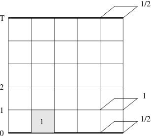
Figure 1: Temporal weight factors of various plaquettes in the Wilson gauge action on a lattice with $T\!=\!5a$ and $L\!=\!5a$.

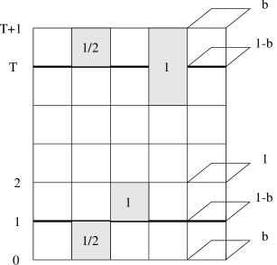
Figure 2: As in fig. 1 for an improved gauge action. The thick lines indicate the inner boundary layers. To avoid classical boundary errors one must choose $b=1/24$.

2.  If the boundary values of the gauge field at the top and bottom of the universe commute, the following is a solution of the lattice field equations for any gauge action: $\bar{U}_{0}(x)=1$, and

$$\bar{U}_{k}(x)=\exp\left({1\over T}\left[x_{0}C^{\prime}_{k}+(T-x_{0})C_{k}\right]\right).$$ (3)

(The boundary values of the gauge field can be read off from the above by evaluating it at $x_{0}=0$ and $T$ for Wilson, respectively, $x_{0}=0,a$ and $T,T+a$ in the improved case.)

The question is if the above background field $\bar{U}$ is the unique (up to gauge equivalence) absolute minimum of the classical action for given boundary values. Uniqueness is important, e.g. for perturbative calculations. A theorem establishing uniqueness holds in the Wilson case [9], if the $C_{k}$, $C_{k}^{\prime}$ parameterizing the boundary values satisfy certain conditions. In the improved case it has been checked using simulated annealing that uniqueness holds under the same conditions [5].

3.  To impose consistent fixed boundary conditions for the fermion fields, it is sufficient to consider the projector structure of the field equations (more precisely, it is only the projector structure in the time direction that matters). For an action with the same projector structure as the standard Wilson quark action, one has to specify $P^{+}\psi(x)$, ${\bar{\psi}}(x)P^{-}$ at the (inner) lower boundary in figs. 1 and 2, and $P^{-}\psi(x)$, ${\bar{\psi}}(x)P^{+}$ at the (inner) upper boundary. Here $P^{\pm}\equiv{\textstyle{1\over 2}}(1\pm\gamma_{0})$. For an improved quark action with the appropriate projector structure [5] one has to specify the same components on both the inner and outer boundary layers in fig. 2.

4.  One of the very useful ideas in applications of the SF is that of quark boundary fields [3]. They are defined as functional derivatives, within the path integral, with respect to the boundary values specified in the previous paragraph (which are then set to zero). For the improved case one can actually define two sets of quark boundary fields. It turns out that if one defines them with respect to the outer boundary values, then most formulas relevant for our application of the SF are identical for improved and standard actions. The boundary fields corresponding to the above boundary values will be denoted as $\bar{\zeta}({\bf x}),\zeta({\bf x}),\bar{\zeta}^{\prime}({\bf x}),\zeta^{\prime}({\bf x})$; the first pair being the lower, the second the upper boundary fields.

5 Details of Non-Perturbative Tuning

With ${\cal O}^{b}=a^{6}\sum_{{\bf y}{\bf z}}\bar{\zeta}({\bf y})\,\gamma_{5}\frac{1}{2}\tau^{b}\zeta({\bf z})$, in terms of the lower boundary fields, and

$$f_{X}(x_{0})\equiv-{1\over V}\sum_{b,{\bf x}}\,{\textstyle{1\over 3}}\,\langle X^{b}(x)\,{\cal O}^{b}\rangle\>,\,X^{b}=A^{b}_{0},P^{b}$$ (4)

the PCAC relation becomes

$$m(x_{0})\equiv r(x_{0})+a\,c_{A}\,s(x_{0})=\widetilde{m}+{\rm O}(a^{2})\,.$$ (5)

where $\widetilde{m}$ differs from $m$ by irrelevant multiplicative renormalization factors, and

$$r(x_{0})\equiv{\nabla_{0}f_{A}(x_{0})\over 2f_{P}(x_{0})}\,,\quad s(x_{0})\equiv{\Delta_{0}f_{P}(x_{0})\over 2f_{P}(x_{0})}\,.$$ (6)

Here $\nabla_{0}$ and $\Delta_{0}$ are standard first and second order lattice derivatives, respectively (in the improved case one actually has to use an improved first order derivative to be consistent).

Similarly, $f^{\prime}_{X},m^{\prime},r^{\prime},s^{\prime}$ are defined in terms of the upper boundary fields $\zeta^{\prime},\bar{\zeta}^{\prime}$.

From $\,m(y_{0})\stackrel{{\scriptstyle!}}{{=}}m^{\prime}(z_{0})\,$ one obtains an estimator of $c_{A}$:

$$\hat{c}_{A}(y_{0},z_{0})~{}\equiv~{}-{1\over a}\,\,{r(y_{0})-r^{\prime}(z_{0})\over s(y_{0})-s^{\prime}(z_{0})}\,.$$ (7)

In terms of a suitable $\hat{c}_{A}$ we now have two different estimates of the current quark mass:

$$M(x_{0}) \,\equiv\, r(x_{0})\,+\,a\,\hat{c}_{A}\,s(x_{0})\,,$$

$$M^{\prime}(x_{0}) \,\equiv\, r^{\prime}(x_{0})\,+\,a\,\hat{c}_{A}\,s^{\prime}(x_{0})\,.$$ (8)

Their equality in the presence of a suitable background field [3, 6] will be our improvement condition for $\omega$. More precisely, we demand

$$\Delta M(x_{0})\equiv M(x_{0})-M^{\prime}(x_{0})\stackrel{{\scriptstyle!}}{{=}}\Delta M^{(0)}(x_{0})$$ (9)

for some well-chosen $x_{0}$; here the superscript $(0)$ denotes the higher order (and small) tree-level value of the quantity in question. In practice one measures the required correlators in a simulation for several trial values of $\omega$, and interpolates to find the zero crossing of $\Delta M-\Delta M^{(0)}$. This determines the non-perturbative value of $\omega$.

6 Results

The results we describe in the following all refer to the SW action on either Wilson or one-loop tadpole improved glue [10, 11] (which we will refer to as “LW glue”). We will always work in the quenched approximation on isotropic lattices.

Below we use some $\hat{c}_{A}(y_{0},y_{0})$ as estimator of $c_{A}$ in eq. (5). We then denote $\Delta M(x_{0})$ by $\Delta M(x_{0},y_{0})$. We used lattices $T\cdot L^{3}=15\cdot 8^{3}$ or $12\cdot 6^{3}$ for Wilson glue, and $14\cdot 8^{3}$ for LW glue. After some study we decided to use $\Delta M(12,4)$ and $\Delta M(9,3)$, respectively, in the improvement condition for $\omega$ in the Wilson case. In the improved case we chose $\Delta M(11,5)$. Typically we generated $1000-2500$ configurations for each gauge coupling considered.

Even though the SF alleviates problems due to zero modes, it turns out that on coarse lattices fluctuations still lead to accidental zero modes at vanishing quark mass (“exceptional configurations”). Fortunately, it turns out that the mass dependence of the non-perturbative $\omega$ is so weak that one can safely determine it at larger mass values. In this manner we have extended the non-perturbative clover coefficient obtained by the ALPHA collaboration for $\beta\geq 6.0$ to $\beta\geq 5.7$. In fig. 3 we illustrate the weak mass (and volume) dependence of $\omega$ for $\beta\!=\!5.7$ Wilson glue. We have also checked that the mass dependence is weak for $\beta\!=\!5.85$ and $6.0$. The same can be seen for LW glue in fig. 4, which furthermore demonstrates the linearity of $\Delta M$ as a function of $\omega$ (all results shown in fig. 4 were calculated using the same gauge configurations).

Figure 3: The non-perturbative clover coefficient $\omega$ for $\beta\!=\!5.7$ Wilson glue for different quark masses and volumes, and its extrapolation to $M\!=\!0$.

Figure 4: Results from the non-perturbative tuning of $\omega$ at different quark masses for LW glue at $\beta_{{\rm LW}}\!=\!8.4$ (where $a\approx 0.1$ fm).

For future use of improved quark actions it is advisable to present the non-perturbative clover coefficient as a definite function of the bare gauge coupling. Combining our Wilson results for $\beta=5.7,5.85$ and $6.0$ with those of the ALPHA collaboration and one-loop perturbation theory we obtain the parameterization ($g^{2}=6/\beta$)

$$\omega(g^{2})={1-0.6050g^{2}-0.1684g^{4}\over 1-0.8709g^{2}}\,,\,\,g^{2}<1.06\,$$ (10)

We were able to accommodate our $\beta=5.7,5.85$ clover coefficients and the value for $\beta=6.2$ from [3] in our curve only in a slightly unsatisfactory manner (extending the Padé in either the numerator or denominator does not help). This issue is under investigation. In the interim the curve (10) should be regarded as preliminary.

For the case of LW glue our current data are parameterized well by

$$\omega_{\rm LW}(g^{2})={1-0.3590\,g^{2}\over 1-0.4784\,g^{2}}\,,\quad g^{2}<1.55\,.$$ (11)

(The one-loop coefficient is presently not known analytically in this case.) The relation between the coefficient of the plaquette term in the LW action, $\beta_{\rm LW}$, and the bare coupling $g^{2}$ is, to one loop [10], $g^{2}=10/(\beta_{\rm LW}-1.422)$. For larger couplings than those in (11) it seems that the non-perturbative $\omega_{\rm LW}$ determined with the SF rises dramatically. This is currently under investigation.

It is interesting to compare the non - perturbative clover coefficients obtained for Wilson and LW glue at the same physical scale. The string tension has been measured for both of these actions, so we will use it to set the scale. We would like a curve parameterizing the string tension $\sigma$ as a function of the coupling. It is known that the two (or three) loop running of the coupling does not properly describe $\sigma$’s lattice spacing dependence (nor that of other observables) for the couplings we are interested in. However, as pointed out in [12], this is not to be expected, since $\sigma$ has discretization errors, $g^{2n}a^{2},a^{4},\ldots$ ($n=0/2$ for Wilson/LW glue) that should be taken into account. We therefore try to parameterize $(a\sqrt{\sigma})(g)$ as

$${\sqrt{\sigma}\over\Lambda}\,f(g^{2})\,\left(\,1+c_{2}\,g^{2n}\,\hat{a}(g)^{2}+c_{4}\,\hat{a}(g)^{4}\,\right),$$ (12)

in terms of the three fit parameters $\sqrt{\sigma}/\Lambda$, $c_{2}$, $c_{4}$. Here $\hat{a}(g)\equiv f(g^{2})/f(1)$, in terms of the universal two-loop function

$$a(g)\Lambda=f(g^{2})\,\equiv\,(b_{0}g^{2})^{-{b_{1}\over 2b_{0}^{2}}}\,\exp(-{1\over 2b_{0}g^{2}})$$ (13)

This works very well (for details see [6]), and the clover coefficients are presented as a function of the lattice spacing in fig. 5. It is interesting to observe that for $a>0.05$ fm both the tadpole and the non-perturbative $\omega$’s are pretty much linear in $a$, at least up to about $0.15$ fm. Furthermore, the differences between the non-perturbative and the tadpole values are essentially linear down to the smallest couplings considered for both cases (of course, for sufficiently small couplings the differences should be of order $g^{2}$).

Figure 5: Non-perturbative clover coefficients versus lattice spacing; scale set by $\sqrt{\sigma}\!=\!460$ MeV. The dashed line denotes the curve from [3]. Small symbols indicate the tree-level (plaquette) tadpole estimates for $\omega$.

7 Conclusions and Outlook

We have shown that the Schrödinger functional and the non-perturbative elimination of ${\rm O}(a)$ errors in a Wilson-type quark action can be successfully extended to improved (gauge) actions. By establishing that the non-perturbative clover coefficient has a very weak mass dependence we were able to determine it for lattice spacings significantly above $0.1$ fm, for both Wilson and improved gauge actions.

We are currently investigating different definitions of the axial current improvement coefficient $c_{A}$. This is necessary if one wants to determine it on coarse lattices, where some definitions lead to a $c_{A}$ of rapidly increasing magnitude (at least when using Wilson glue). Once the $c_{A}$ determination is completed we plan to determine the other current normalization and improvement coefficients [3].

There are many other situations in which the non-perturbative elimination of the ${\rm O}(a)$ violations of chiral symmetry is important, the most obvious examples being full QCD and D234 quarks on anisotropic lattices (for the study of heavy quarks). We hope that the ultimate outcome of this and future studies will be the ability to perform accurate continuum extrapolations from much coarser, and therefore cheaper, lattices than hitherto possible.

References

- [1] K. Symanzik, Nucl. Phys. B226 (1983) 187.
- [2] G.P. Lepage and P.B. Mackenzie, Phys. Rev. D48 (1993) 2250.
- [3] M. Lüscher et al, Nucl. Phys. B491 (1997) 323, 344.
- [4] B. Sheikholeslami and R. Wohlert, Nucl. Phys. B259 (1985) 572.
- [5] T.R. Klassen, hep-lat/9705025, Nucl. Phys. B, in press.
- [6] R.G. Edwards, U.M. Heller and T.R. Klassen, in preparation.
- [7] M. Alford, T.R. Klassen and G.P. Lepage, these proceedings.
- [8] M. Alford, T.R. Klassen and G.P. Lepage, Nucl. Phys. B496 (1997) 377; Nucl. Phys. B (Proc. Suppl.) 47 (1996) 370; 53 (1997) 861.
- [9] M. Lüscher, R. Narayanan, P. Weisz, and U. Wolff, Nucl. Phys. B384 (1992) 168.
- [10] M. Lüscher and P. Weisz, Comm. Math. Phys. 97 (1985) 59; Phys. Lett. 158B (1985) 250.
- [11] M. Alford et al, Phys. Lett. B361 (1995) 87.
- [12] C. Allton, hep-lat/9610016.