KEK-CP-063 October 1997 Scaling Study of the Two-Flavor Chiral Phase Transition with the Kogut-Susskind Quark Action in Lattice QCD

Abstract

We report on a study of two-flavor finite-temperature chiral phase transition employing the Kogut-Susskind quark action and the plaquette gluon action in lattice QCD for a lattice with $N_{t}=4$ temporal size. Hybrid R simulations of $10^{4}$ trajectories are made at quark masses of $m_{q}=0.075,0.0375,0.02,0.01$ in lattice units for the spatial sizes $8^{3},12^{3}$ and $16^{3}$. The spatial size dependence of various susceptibilities confirm the previous conclusion of the absence of a phase transition down to $m_{q}=0.02$. At $m_{q}=0.01$ an increase of susceptibilities is observed up to the largest volume $16^{3}$ explored in the present work. We argue, however, that this increase is likely to be due to an artifact of too small a lattice size and it cannot be taken to be the evidence for a first-order transition. Analysis of critical exponents estimated from the quark mass dependence of susceptibilities shows that they satisfy hyperscaling consistent with a second-order transition located at $m_{q}=0$. The exponents obtained from larger lattice, however, deviate significantly from both those of O(2), which is the exact symmetry group of the Kogut-Susskind action at finite lattice spacing, and those of O(4) expected from an effective sigma model analysis in the continuum limit.

1 Introduction

The nature of the finite-temperature chiral phase transition has been pursued using lattice QCD over many years. The commonly adopted simplification is to approximate the real world with $N_{f}$ flavors of degenerate quarks. Theoretical arguments[3] based on an effective sigma model that preserves chiral symmetry of QCD suggest the order of the transition changing from first to probably second as $N_{f}$ decreases from $N_{f}\geq 3$ to $N_{f}=2$, which is a reasonably close approximation to reality.

Lattice QCD simulations with the Kogut-Susskind quark action have shown that the transition is indeed of first order for $N_{f}=4$[4, 5, 6, 7]. There are indications, though much less extensive, that the $N_{f}=3$ transition is also of first order[8] in agreement with the theoretical expectation. A physically important case of $N_{f}=2$, on the other hand, has turned out to be more elusive. In Ref. [7] a finite-size scaling analysis was attempted at quark masses $m_{q}=0.025$ and 0.0125 in lattice units for a temporal lattice size of $N_{t}=4$ employing the spatial sizes $6^{3}$, $8^{3}$ and $12^{3}$. While the results clearly confirmed that the $N_{f}=2$ transition is much weaker than that for $N_{f}=4$, a first-order transition could not be quite excluded since various susceptibilities exhibited some increase with spatial volume up to $12^{3}$. Simulations on a $16^{3}\times 4$ lattice at $m_{q}=0.025$ and 0.01 carried out by the Columbia group[8] showed, however, that the susceptibilities flatten off between $12^{3}$ and $16^{3}$ spatial sizes. The combined results led to the conclusion that a phase transition is absent down to the quark mass of $m_{q}\approx 0.01-0.0125$, and this was taken to be consistent with the prediction of the sigma model analysis[3] for a second-order transition which takes place at $m_{q}=0$, and changes into a crossover at $m_{q}\neq 0$.

If the $N_{f}=2$ transition is indeed to follow the prediction of the effective sigma model, critical exponents for the $N_{f}=2$ system should agree with those of the O(4) Heisenberg model in three dimensions. This point was first studied by Karsch[9]. Examining world data for the critical coupling $\beta_{c}(m_{q})$ as a function of quark mass $m_{q}$, he concluded that the dependence is consistent with a second-order scaling behavior with the O(4) critical exponents. This analysis has been extended in Ref. [10] in which various susceptibilities were measured on an $8^{3}\times 4$ lattice at $m_{q}=0.075,0.0375,0.02$, and critical exponents were extracted from the quark mass dependence of the peak height of susceptibilities. The results showed that the magnetic exponent was in fair agreement with the O(4) value, while that for the thermal exponent exhibited a sizable deviation.

In these earlier analyses there are a number of respects that deserve further investigations. First, the conclusion on the absence of a first-order transition at $m_{q}\approx 0.01$ from finite size scaling was based on a combination of finite-size data from two groups[7, 8] which employed slightly different quark masses ($m_{q}=0.0125$[7] and $0.01$[8]). There is also a suspicion that the simulation may not be long enough. It is clearly desirable to reexamine finite-size scaling behavior with a homogeneous data set generated under the same simulation conditions. Second, the method of second-order scaling analysis should be applicable only for sufficiently large lattice sizes to avoid finite-size effects. It is not clear if the spatial size of $8^{3}$ employed by Karsch and Laermann[10] is sufficient, especially toward light quark masses. Additional question is whether the range of quark mass $m_{q}=0.075-0.02$ they explored is small enough for the true critical behavior to manifest in the susceptibilities. Thus an extension of their work toward larger spatial sizes and smaller quark masses is undoubtfully desired.

In order to address these points we have carried out new simulations for the two-flavor chiral phase transition with the Kogut-Susskind quark action, and systematically collected data over a range of spatial sizes and quark masses with statistics higher than in the previous work. Our simulations have been made for $m_{q}=0.075$, $0.0375$, $0.02$ and $0.01$ on lattices of size $8^{3}\times 4$, $12^{3}\times 4$ and $16^{3}\times 4$, accumulating 10000 trajectories of the hybrid R algorithm for each parameter set. In this article we present details of the runs and results of our analyses on both finite-size and second-order scaling behavior. The calculations have been performed on the Fujitsu VPP500/80 supercomputer at KEK.

A preliminary account of our results was reported in Ref. [11]. A similar study has been carried out by the Bielefeld group[12] with lattice sizes up to $16^{3}\times 4$ but keeping the quark mass only to $m_{q}\geq 0.02$. The MILC Collaboration has recently started simulations for small quark masses down to $m_{q}=0.008$ employing lattices as large as $24^{3}$[13].

In Sec. 2 we describe details of our simulation. In particular we explain our method for computing the disconnected part of fermionic susceptibilities which is non-trivial. In Sec. 3 we discuss finite-size scaling analysis for a given quark mass. In Sec. 4 analyses of exponents and scaling functions extracted from the quark mass dependence of susceptibilities are presented. Conclusions of the present work are given in Sec. 5.

2 Simulation and measurements

2.1 Simulation algorithm

The present study is carried out with the plaquette action for gluons and the Kogut-Susskind action for quarks. The effective action is given by

$$S_{eff}=-\frac{\beta}{6}\sum_{plaquette}\mbox{Tr}\left(U_{plaquette}\right)-\frac{N_{f}}{4}\mbox{Tr}\log\left(D(U)^{\dagger}D(U)\right)_{e},$$ (1)

where $N_{f}=2$, the subscript $e$ means the even part, and $D(U)$ denotes the Kogut-Susskind quark operator,

$$D(U)=m_{q}+\frac{1}{2}\sum_{\mu}D_{\mu}(U)$$ (2)

with

$$D_{\mu}(U)_{x,y}=\eta_{x\mu}\left(U_{x\mu}\delta_{x+\hat{\mu},y}U_{x\mu}-\delta_{x-\hat{\mu},y}U_{y\mu}^{\dagger}\right).$$ (3)

We employ the standard hybrid R algorithm to simulate the system, adopting the same normalization of the step size $\Delta\tau$ as in the original literature[14]. In the leap-frog update to solve the molecular dynamics equations, link variables are assigned to half-integer time steps and conjugate momenta to integer times. Inversion of the quark operator is made with the conjugate gradient algorithm.

2.2 Observables and method of measurement

We consider local observables defined by

$$\overline{\psi}\psi = \frac{1}{V}\sum_{x}\overline{\psi}_{x}\psi_{x},$$ (4)

$$\overline{\psi}D_{0}\psi = \frac{1}{V}\sum_{x,y}\overline{\psi}_{x}D_{0x,y}\psi_{y},$$ (5)

$$P_{\tau} = \frac{1}{9V}\sum_{x}\sum_{1\leq i\leq 3}\mbox{Tr}\left(U_{x4i}\right),$$ (6)

$$P_{\sigma} = \frac{1}{9V}\sum_{x}\sum_{1\leq i<j\leq 3}\mbox{Tr}\left(U_{xij}\right),$$ (7)

$$\Omega = \frac{1}{L^{3}}\sum_{\vec{x}}\Omega_{\vec{x}},\qquad\Omega_{\vec{x}}=\frac{1}{3}\mbox{Tr}\left(\prod_{x_{t}=1}^{N_{t}}U_{x4}\right),$$ (8)

where $V=L^{3}\cdot N_{t}$ denotes the lattice volume of an $L^{3}\times N_{t}$ lattice, $D_{0}$ the temporal hopping term of the Kogut-Susskind operator as defined in (3), and $U_{x\mu\nu}$ the plaquette in the $\mu\nu$ plane. In the course of our simulation, we measure these quantities and the corresponding susceptibilities given by

$$\chi_{m} = V\left[\langle\left(\overline{\psi}\psi\right)^{2}\rangle-\langle\overline{\psi}\psi\rangle^{2}\right],$$ (9)

$$\chi_{t,f} = V\left[\langle\left(\overline{\psi}\psi\right)\left(\overline{\psi}D_{0}\psi\right)\rangle-\langle\overline{\psi}\psi\rangle\langle\overline{\psi}D_{0}\psi\rangle\right],$$ (10)

$$\chi_{t,i} = V\left[\langle\left(\overline{\psi}\psi\right)P_{i}\rangle-\langle\overline{\psi}\psi\rangle\langle P_{i}\rangle\right],\qquad i=\sigma,\tau,$$ (11)

$$\chi_{e,f} = V\left[\langle\left(\overline{\psi}D_{0}\psi\right)^{2}\rangle-\langle\overline{\psi}D_{0}\psi\rangle^{2}\right],$$ (12)

$$\chi_{e,i} = V\left[\langle\left(\overline{\psi}D_{0}\psi\right)P_{i}\rangle-\langle\overline{\psi}D_{0}\psi\rangle\langle P_{i}\rangle\right],\qquad i=\sigma,\tau,$$ (13)

$$\chi_{e,ij} = V\left[\langle P_{i}P_{j}\rangle-\langle P_{i}\rangle\langle P_{j}\rangle\right],\qquad i,j=\sigma,\tau,$$ (14)

$$\chi_{\Omega} = V\left[\langle\Omega^{2}\rangle-\langle\Omega\rangle^{2}\right].$$ (15)

Calculation of the fermionic susceptibilities $\chi_{m}$, $\chi_{t,f}$ and $\chi_{e,f}$ is non-trivial because of the presence of disconnected quark loop contributions. Let us illustrate our procedure for $\chi_{m}$. After quark contractions and correcting by powers of $N_{f}/4$ for normalization to $N_{f}$ flavors, $\chi_{m}$ is written

$$\chi_{m} = \chi_{disc}+\chi_{conn},$$ (16)

$$\chi_{disc} = \left(\frac{N_{f}}{4}\right)^{2}\frac{1}{V}\left[\langle\left(\mbox{Tr}D^{-1}\right)^{2}\rangle-\langle\mbox{Tr}D^{-1}\rangle^{2}\right],$$ (17)

$$\chi_{conn} = -\frac{N_{f}}{4}\frac{1}{V}\sum_{x,y}\langle D_{x,y}^{-1}D_{y,x}^{-1}\rangle.$$ (18)

We employ the volume source method without gauge fixing[15] to evaluate the two parts. Let

$$G_{x}^{a,b}\equiv\sum_{y}\left(D^{-1}\right)_{x,y}^{a,b}$$ (19)

be the quark propagator for unit source placed at every space-time site with a given color $b$. Define

$$O_{1} = \sum_{x,y}\sum_{a,b}G_{x}^{a,a}G_{y}^{b,b},$$ (20)

$$O_{2} = \sum_{x,y}\sum_{a,b}G_{x}^{a,b}G_{y}^{b,a},$$ (21)

$$O_{3} = \sum_{x}\sum_{a,b}G_{x}^{a,a}G_{x}^{b,b},$$ (22)

$$O_{4} = \sum_{x}\sum_{a,b}G_{x}^{a,b}G_{x}^{b,a}.$$ (23)

Up to terms which are gauge non-invariant, and hence vanish on the average, we find

$$\left(\mbox{Tr}D^{-1}\right)^{2} = +\frac{9}{8}O_{1}-\frac{3}{8}O_{2}-\frac{1}{8}O_{3}+\frac{3}{8}O_{4},$$ (24)

$$\sum_{x,y}D_{x,y}^{-1}D_{y,x}^{-1} = -\frac{3}{8}O_{1}+\frac{9}{8}O_{2}+\frac{3}{8}O_{3}-\frac{1}{8}O_{4}.$$ (25)

Note that $O_{1}$ contains the connected contribution in addition to the dominant disconnected part, and vice versa for $O_{2}$. The terms $O_{3}$ and $O_{4}$ represent contact contributions in which the source and sink points of quark coincide.

To calculate the susceptibility $\chi_{t,f}$ we need to replace one of the volume source propagator $G_{x}^{a,b}$ in (20–23) by $(D_{0}G)_{x}^{a,b}$. Both propagators should be replaced in this way for $\chi_{e,f}$.

2.3 Choice of run parameters

The distribution of observables generated by the hybrid R algorithm suffers from systematic errors arising from a finite molecular dynamics step size $\Delta\tau$ and a finite stopping condition taken for the conjugate gradient inversion of the quark operator. For analyses of critical properties of phase transitions, potential problems caused by these systematic errors are a shift of the critical coupling $\beta_{c}$ and a modification of susceptibilities, in particular a change in the magnitude of the peak height of susceptibilities at $\beta=\beta_{c}$. In order to examine these effects we carry out test runs on an $8^{3}\times 4$ lattice at $m_{q}=0.02$.

Figure 1: Time history of chiral order parameter for a series of values of the stopping condition on an $8^{3}\times 4$ lattice at $m_{q}=0.02$ and $\Delta\tau=0.03$.

Let us define a residual $r$ of the conjugate gradient inversion algorithm applied for a source vector $b$ by

$$r\equiv\sqrt{\frac{||b_{e}-(D^{\dagger}Dx)_{e}||^{2}}{3V}},$$ (26)

where, as in (1), the subscript $e$ means the even part. The choice of the factor $3V$ is motivated by the fact that the norm of the residue vector $||b_{e}-(D^{\dagger}Dx)_{e}||^{2}$ is proportional to $V=L^{3}\cdot N_{t}$ for a Gaussian noise source employed for the hybrid R algorithm.

To test effects of the stopping condition, we choose an approximate value of the critical coupling $\beta=5.282$ for $m_{q}=0.02$, and generate 1000 trajectories of unit length with a fixed step size of $\Delta\tau=0.03$, varying the stopping condition from $r=10^{-2}$ to $10^{-6}$. The time histories of the chiral order parameter $\overline{\psi}\psi$ for the runs are shown in Fig 1. We observe that a looser stopping condition leads to a smaller value and a larger magnitude of fluctuations of $\overline{\psi}\psi$. The results, however, are stable for $r\hbox to0.0pt{\lower 3.5pt\hbox{$\mathchar 0\relax\sim$}\hss}\raise 1.0pt\hbox{$<$}10^{-4}-10^{-5}$. In all of our production runs we therefore take the condition given by

$$r<10^{-6}.$$ (27)

Another possible measure of the stopping condition is to employ the ratio

$$\tilde{r}=\frac{||b_{e}-(D^{\dagger}Dx)_{e}||}{||x_{e}||}.$$ (28)

With a Gaussian noise source we expect $||x_{e}||^{2}\propto c(m_{q})V$ with the coefficient $c(m_{q})$ increasing as $m_{q}$ becomes smaller. Thus our stopping condition is relatively tighter toward smaller quark masses compared to that given in terms of (28).

We examine systematic effects of the step size by carrying out runs of $10000$ trajectories of unit length for the combinations $(\beta,\Delta\tau)=(5.282,0.01)$, $(5.284,0.014)$, $(5.284,0.02)$ with the stopping condition fixed at $r=10^{-6}$.

Figure 2: (a) Critical coupling as a function of step size. (b) Peak height of $\chi_{m}$ as a function of step size. Data are taken on an $8^{3}\times 4$ lattice at $m_{q}=0.02$ with $r<10^{-6}$.

The critical coupling $\beta_{c}(\Delta\tau)$ estimated from the peak position of the chiral susceptibility $\chi_{m}$, and its peak height $\chi_{m}^{max}(\Delta\tau)$ are plotted in Fig. 2(a) and (b) as a function of $\Delta\tau^{2}$, where the standard reweighting technique[16] is employed to estimate $\beta_{c}(\Delta\tau)$ and $\chi_{m}^{max}(\Delta\tau)$. We observe that the results are consistent with an $O(\Delta\tau^{2})$ dependence theoretically expected[14, 17, 18]. Since quark mass is expected to affect the systematic error in the combination $(\Delta\tau/m_{q})^{2}$, we parametrize $\beta_{c}(\Delta\tau)$ and $\chi_{m}^{max}(\Delta\tau)$ in the form $a(1+c(\Delta\tau/m_{q})^{2})$ and find $a=5.2812(26)$, $c=0.0011(6)$ for $\beta_{c}(\Delta\tau)$ and $a=14.1(1.2)$, $c=0.34(16)$ for $\chi_{m}^{max}(\Delta\tau)$. These values suggest that choosing $\Delta\tau\approx\frac{m_{q}}{2}$ leads to an accuracy of 0.03% (or $0.0015$ in magnitude) for $\beta_{c}$ and 9% for $\chi_{m}^{max}$. We think these accuracies to be sufficient compared to our statistical errors, and adopt $\Delta\tau\approx\frac{m_{q}}{2}$ for our production runs.

2.4 Summary of runs

We carry out runs for the temporal lattice size $N_{t}=4$ at the quark masses $m_{q}=0.075,0.0375,0.02$ and $0.01$. For each quark mass we employ three spatial lattice sizes given by $L=8,12$ and $16$. For each set $(m_{q},L)$ we choose a single value of $\beta$ close to the critical coupling, which is selected by preliminary short runs, and carry out a long simulation of 10000 trajectories of unit length starting from an ordered configuration using the stopping condition as described in Sec. 2.3. Variation of observables as a function of $\beta$ is calculated by the reweighting technique[16] from a single run.

In applying the reweighting technique one may consider an alternative procedure of making a number of shorter runs for a set of values of $\beta$ around $\beta_{c}$. In practice we find long-range fluctuations of $O(1000)$ trajectories toward smaller quark masses and larger volumes, so that a simulation at a single parameter point is already quite computer time intensive to get rid of these fluctuations. We therefore adopt the approach of making a single long run at a well-chosen value of $\beta$ in the present work.

In Table 1 we list the values of $\beta$ where our runs are carried out and the molecular dynamics step size $\Delta\tau$ used. Two runs are made for $m_{q}=0.01$ on a $12^{3}\times 4$ lattice since the first run at $\beta=5.266$ turns out to be predominantly in the low-temperature phase. We collect time histories of the chiral order parameter $\overline{\psi}\psi$ and their histograms in Fig 3.

$(a)\quad m_{q}=0.075$

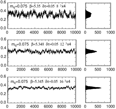
$(b)\quad m_{q}=0.0375$

Figure 3: Time history of $\overline{\psi}\psi$ and histograms of the runs.

$(c)\quad m_{q}=0.02$

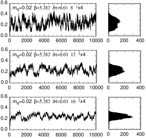
$(d)\quad m_{q}=0.01$

Figure 3: Continued

In all of the runs observables are calculated at every trajectory, discarding the initial 2000 trajectories of each run. Jackknife analysis is carried out for the reminaing 8000 trajectories to estimate errors. Examining the bin size of 400 and 800 we find that the magnitude of errors is stable, and we adopt 800 for the bin size of our error estimations.

Table 1: Parameters of our runs. For each parameter point 10000 trajectories are generated with the stopping condition $r=10^{-6}$ for the conjugate gradient solver.

$N_{s}$	$m_{q}=0.075$	$0.0375$	$0.02$	$0.01$
	$\Delta\tau=0.05$	0.02	0.01	0.005
8	$\beta=5.35$	5.306	5.282	5.266
12	$\beta=5.348$	5.306	5.282	5.266
				5.2665
16	$\beta=5.345$	5.306	5.282	5.266

Table 2: Peak position $\beta_{c}$ and peak height $\chi^{max}$ of various susceptibilities for each quark mass $m_{q}$ and spatial lattice size $L$.

	$L=8$		$L=12$		$L=16$
$m_{q}$	$\beta_{c}$	$\chi_{m}^{max}$	$\beta_{c}$	$\chi_{m}^{max}$	$\beta_{c}$	$\chi_{m}^{max}$
0.0750	5.3494(17)	5.9(0.3)	5.3477(14)	6.3(0.6)	5.3443(18)	6.3(0.7)
0.0375	5.3073(18)	10.5(0.5)	5.3099(16)	11.6(1.6)	5.3072(7)	14.1(2.2)
0.0200	5.2831(23)	14.7(1.0)	5.2823(8)	24.6(3.1)	5.2819(5)	22.9(2.2)
0.0100	5.2665(20)	24.4(1.6)	5.2681(7)	44.4(6.2)	5.2657(4)	63.9(12.3)
0.0100			5.2665(6)	38.0(3.9)
$m_{q}$	$\beta_{c}$	$\chi_{t,f}^{max}$	$\beta_{c}$	$\chi_{t,f}^{max}$	$\beta_{c}$	$\chi_{t,f}^{max}$
0.0750	5.3484(17)	-1.97(0.13)	5.3472(12)	-2.08(0.24)	5.3441(14)	-2.17(0.24)
0.0375	5.3064(19)	-2.76(0.16)	5.3086(14)	-3.20(0.43)	5.3069(7)	-4.11(0.72)
0.0200	5.2821(18)	-3.23(0.27)	5.2819(9)	-5.82(0.77)	5.2817(5)	-5.71(0.56)
0.0100	5.2658(20)	-4.77(0.39)	5.2678(7)	-9.02(1.31)	5.2655(4)	-14.05(3.25)
0.0100			5.2661(7)	-8.20(0.89)
$m_{q}$	$\beta_{c}$	$\chi_{t,\sigma}^{max}$	$\beta_{c}$	$\chi_{t,\sigma}^{max}$	$\beta_{c}$	$\chi_{t,\sigma}^{max}$
0.0750	5.3483(16)	-0.71(0.05)	5.3474(14)	-0.76(0.10)	5.3441(16)	-0.80(0.11)
0.0375	5.3060(19)	-1.04(0.07)	5.3085(19)	-1.15(0.17)	5.3069(8)	-1.48(0.27)
0.0200	5.2816(22)	-1.24(0.11)	5.2819(9)	-2.22(0.29)	5.2816(6)	-2.12(0.22)
0.0100	5.2656(22)	-1.91(0.15)	5.2679(7)	-3.70(0.57)	5.2656(4)	-5.62(1.17)
0.0100			5.2661(7)	-3.18(0.39)
$m_{q}$	$\beta_{c}$	$\chi_{t,\tau}^{max}$	$\beta_{c}$	$\chi_{t,\tau}^{max}$	$\beta_{c}$	$\chi_{t,\tau}^{max}$
0.0750	5.3482(16)	-0.79(0.06)	5.3473(14)	-0.84(0.11)	5.3439(17)	-0.89(0.12)
0.0375	5.3061(19)	-1.16(0.08)	5.3088(22)	-1.29(0.22)	5.3069(8)	-1.68(0.32)
0.0200	5.2817(22)	-1.40(0.12)	5.2819(9)	-2.53(0.33)	5.2816(6)	-2.41(0.25)
0.0100	5.2656(21)	-2.12(0.17)	5.2679(7)	-4.09(0.63)	5.2656(4)	-6.32(1.35)
0.0100			5.2661(7)	-3.56(0.42)
$m_{q}$	$\beta_{c}$	$\chi_{e,f}^{max}$	$\beta_{c}$	$\chi_{e,f}^{max}$	$\beta_{c}$	$\chi_{e,f}^{max}$
0.0750	5.3480(17)	1.31(0.06)	5.3462(16)	1.41(0.10)	5.3441(13)	1.38(0.09)
0.0375	5.3062(25)	1.53(0.06)	5.3078(15)	1.55(0.11)	5.3065(7)	1.96(0.25)
0.0200	5.2825(19)	1.60(0.11)	5.2813(13)	2.09(0.18)	5.2815(10)	2.18(0.18)
0.0100	5.2626(31)	2.14(0.19)	5.2676(9)	2.39(0.34)	5.2656(4)	3.82(0.84)
0.0100			5.2657(6)	2.58(0.31)
$m_{q}$	$\beta_{c}$	$\chi_{e,\sigma}^{max}$	$\beta_{c}$	$\chi_{e,\sigma}^{max}$	$\beta_{c}$	$\chi_{e,\sigma}^{max}$
0.0750	5.3478(17)	0.236(0.021)	5.3470(14)	0.259(0.040)	5.3441(15)	0.271(0.041)
0.0375	5.3058(21)	0.276(0.021)	5.3080(18)	0.321(0.050)	5.3067(8)	0.438(0.088)
0.0200	5.2813(20)	0.279(0.031)	5.2816(9)	0.538(0.076)	5.2815(7)	0.530(0.059)
0.0100	5.2652(21)	0.399(0.032)	5.2677(7)	0.754(0.120)	5.2655(4)	1.245(0.314)
0.0100			5.2658(7)	0.715(0.089)

Table 2: Continued

$m_{q}$	$\beta_{c}$	$\chi_{e,\tau}^{max}$	$\beta_{c}$	$\chi_{e,\tau}^{max}$	$\beta_{c}$	$\chi_{e,\tau}^{max}$
0.0750	5.3477(17)	0.302(0.025)	5.3470(14)	0.321(0.043)	5.3439(16)	0.335(0.045)
0.0375	5.3059(20)	0.351(0.023)	5.3082(19)	0.399(0.060)	5.3067(8)	0.539(0.100)
0.0200	5.2812(19)	0.358(0.032)	5.2816(9)	0.659(0.085)	5.2815(7)	0.642(0.066)
0.0100	5.2652(21)	0.487(0.039)	5.2677(7)	0.871(0.133)	5.2655(4)	1.440(0.362)
0.0100			5.2658(7)	0.834(0.098)
$m_{q}$	$\beta_{c}$	$\chi_{e,\sigma\sigma}^{max}$	$\beta_{c}$	$\chi_{e,\sigma\sigma}^{max}$	$\beta_{c}$	$\chi_{e,\sigma\sigma}^{max}$
0.0750	5.3478(15)	0.141(0.008)	5.3474(14)	0.149(0.015)	5.3443(14)	0.159(0.019)
0.0375	5.3053(21)	0.161(0.010)	5.3075(22)	0.170(0.020)	5.3067(9)	0.212(0.033)
0.0200	5.2808(23)	0.162(0.013)	5.2816(9)	0.261(0.028)	5.2814(7)	0.252(0.023)
0.0100	5.2650(22)	0.214(0.016)	5.2678(8)	0.369(0.053)	5.2655(5)	0.557(0.111)
0.0100			5.2658(7)	0.331(0.040)
$m_{q}$	$\beta_{c}$	$\chi_{e,\sigma\tau}^{max}$	$\beta_{c}$	$\chi_{e,\sigma\tau}^{max}$	$\beta_{c}$	$\chi_{e,\sigma\tau}^{max}$
0.0750	5.3479(15)	0.135(0.010)	5.3474(14)	0.143(0.018)	5.3441(16)	0.152(0.021)
0.0375	5.3055(21)	0.155(0.010)	5.3079(24)	0.166(0.024)	5.3067(9)	0.218(0.039)
0.0200	5.2809(23)	0.157(0.014)	5.2816(10)	0.272(0.032)	5.2814(6)	0.262(0.026)
0.0100	5.2651(22)	0.214(0.018)	5.2678(7)	0.385(0.058)	5.2655(5)	0.600(0.127)
0.0100			5.2658(7)	0.345(0.043)
$m_{q}$	$\beta_{c}$	$\chi_{e,\tau\tau}^{max}$	$\beta_{c}$	$\chi_{e,\tau\tau}^{max}$	$\beta_{c}$	$\chi_{e,\tau\tau}^{max}$
0.0750	5.3477(16)	0.168(0.012)	5.3473(13)	0.175(0.020)	5.3438(18)	0.186(0.024)
0.0375	5.3055(20)	0.189(0.011)	5.3083(27)	0.202(0.030)	5.3067(9)	0.265(0.046)
0.0200	5.2809(22)	0.194(0.015)	5.2816(10)	0.326(0.036)	5.2814(6)	0.314(0.030)
0.0100	5.2650(22)	0.254(0.019)	5.2678(7)	0.442(0.065)	5.2655(5)	0.689(0.146)
0.0100			5.2659(7)	0.403(0.047)
$m_{q}$	$\beta_{c}$	$\chi_{\Omega}^{max}$	$\beta_{c}$	$\chi_{\Omega}^{max}$	$\beta_{c}$	$\chi_{\Omega}^{max}$
0.0750	5.3479(19)	4.21(0.28)	5.3462(13)	4.52(0.51)	5.3439(14)	4.63(0.54)
0.0375	5.3064(20)	4.10(0.25)	5.3087(15)	4.53(0.57)	5.3068(7)	6.05(1.03)
0.0200	5.2823(20)	3.73(0.32)	5.2819(9)	6.30(0.75)	5.2817(5)	6.17(0.62)
0.0100	5.2655(22)	4.45(0.34)	5.2677(8)	8.06(1.17)	5.2655(4)	12.57(3.00)
0.0100			5.2660(7)	7.21(0.78)

3 Analysis of spatial volume dependence

3.1 Finite-size scaling analysis

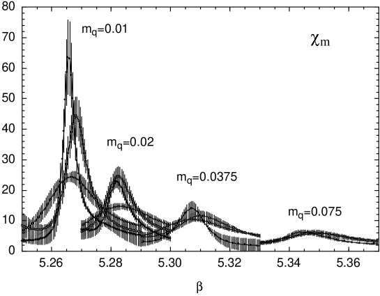
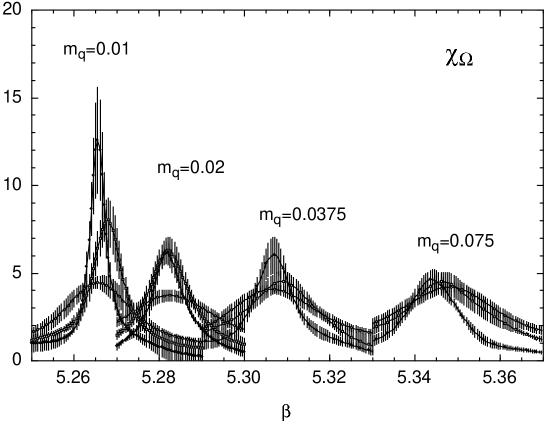
Figure 4: (a) Chiral susceptibility $\chi_{m}$ as a function of $\beta$. (b) Same for the Polyakov susceptibility $\chi_{\Omega}$. For $L=12$ at $m_{q}=0.01$ the run with $\beta=5.266$ is employed.

We start our analysis with an examination of the spatial volume dependence of susceptibilities for each quark mass. The $\beta$ dependence of susceptibilities, evaluated with the reweighting technique for each $m_{q}$ and spatial size $L$, is illustrated for the chiral and Polyakov susceptibilities, $\chi_{m}$ and $\chi_{\Omega}$, in Fig 4. Let us denote by $\beta_{c}$ and $\chi^{max}$ the position and height of the peak of a susceptibility. Our numerical results for these quantities are summarized in Table 2 for each of the susceptibilities defined by (9–15). As typical examples, we plot $\chi_{m}^{max}$, $\chi_{t,f}^{max}$ and $\chi_{\Omega}^{max}$ as a function of spatial volume $L^{3}$ in Fig 5. Two points for $m_{q}=0.01$ on a $12^{3}$ lattice represent two runs at these parameters. The agreement between the two points justifies the robustness of the reweighting method: the method works well even if the simulation is carried out in one side of the two phases, i.e., at $\beta$ off the critical value. The behavior of other susceptibilities are similar as one may find from Table 2.

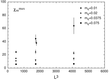
Figure 5: Peak height of the susceptibility $\chi_{m}$, $\chi_{t,f}$ and $\chi_{\Omega}$ as a function of spatial volume $L^{3}$.

For the heavier quark masses of $m_{q}=0.075$ and 0.0375 the peak height of the susceptibilities increases little over the sizes $L=8-16$, showing that a phase transition is absent for these masses. For $m_{q}=0.02$, a significant increase is seen between $L=8$ and 12. The increase, however, does not continue beyond $L=12$, with the peak height for $L=16$ consistent with that for $L=12$. We then conclude an absence of a phase transition also for $m_{q}=0.02$. The histogram shown in Fig. 3(c) provides further support for this conclusion; while the histogram for the size $L=8$ is broad and even hint at a possible presence of a double peak structure, such an indication for metastability is less visible for $L=12$, and a single peak structure becomes quite manifest for $L=16$.

For $m_{q}=0.01$ the peak height also increases between $L=8$ and 12. Furthermore, the increase continues up to $L=16$. In fact the rate of increase is consistent with a linear behavior in volume, which is expected for a first-order phase transition.

We think, however, that caution must be exercised to draw a conclusion solely from Fig 5. Comparing the time histories of $\overline{\psi}\psi$ for the three lattice sizes $L=8$, $12$ and $16$ in Fig 3(d), we observe that a flip-flop behavior between two different values of $\overline{\psi}\psi$ is most distinct for the smallest lattice size $L=8$, and the time histories for the larger lattice sizes $L=12$ and 16 are dominated more by irregular patterns, the width of fluctuations becoming smaller as the size increases. These features are also reflected in the histograms. A double-peak distribution, clearly seen for $L=8$, is less evident for $L=12$ and barely visible for $L=16$. Moreover, the width of the distribution is narrower for larger lattice sizes. These trends show a marked contrast with the case of the first-order deconfining phase transitions of the pure SU(3) gauge theory and of four-flavor QCD, where a flip-flop behavior in the time history and a double-peak distribution in histograms become progressively pronounced toward larger spatial volumes, for instance, as is seen in Fig. 1 of Ref. [19].

The observations above indicate that the increase of susceptibilities seen for $m_{q}=0.01$ is due to insufficient spatial volume, which is similar to an increase between $L=8$ and $12$ for $m_{q}=0.02$ for which the susceptibilities level off for $L=16$. In order to make a comparison of volume dependence for different quark masses, we need to normalize the lattice size in terms of a relevant length scale, which may be taken to be the pion correlation length $\xi_{\pi}=1/m_{\pi}$ at zero temperature. Results of $m_{\pi}$ precisely at the values of $\beta$ and $m_{q}$ where our simulations are made are not available. The MILC Collaboration, however, has given a parametrization of available data for $\pi$ and $\rho$ meson masses as a function of $\beta$ and $m_{q}$[18], from which we find $\xi_{\pi}\approx 3.0$ for $m_{q}=0.02$ and $\xi_{\pi}\approx 4.4$ for $m_{q}=0.01$ at the respective critical couplings. Hence the size $L=8$ for $m_{q}=0.02$ roughly corresponds to $L=12$ for $m_{q}=0.01$, and $L=12$ to $L=16$. Comparing the histograms for $m_{q}=0.02$ and $0.01$ which are in correspondence in this sense, we find that they are similar not only in shape but also in the trend that a double peak type distribution changes toward that of a single peak for larger sizes.

Figure 6: Peak height of chiral susceptibility $\chi_{m}$ as a function of spatial size $L$, both normalized by zero-temperature pion mass $m_{\pi}$.

A more quantitative comparison is made in Fig. 6 where we plot the dimensionless combination $\chi_{m}^{max}\cdot m_{\pi}^{2}$ against $Lm_{\pi}$. Data points for various quark masses and spatial sizes roughly fall on a single curve, and the increase observed up to $L=16$ for $m_{q}=0.01$ does not stand out as particularly large. It is quite plausible that the peak height for $m_{q}=0.01$ levels off if measured on a larger lattice, e.g., $L=24$.

While a definitive conclusion has to await simulations on larger spatial sizes, our examinations lead us to conclude that a first-order phase transition is absent also at $m_{q}=0.01$.

3.2 Comparison with previous studies

Finite-size analyses similar to those reported here were previously carried out by two groups[7, 8]. In Ref. [7] runs of $4000-10000$ trajectories of unit length were made for the spatial sizes $6^{3}$, $8^{3}$ and $12^{3}$ at $m_{q}=0.0125$ and $0.025$ using the step size of $\Delta\tau=0.02$ for both cases. In Ref. [8] a larger spatial lattice of $16^{3}$ was employed, and 2500 trajectories were generated at $m_{q}=0.01(\Delta\tau=0.0078)$ and $m_{q}=0.025(\Delta\tau=0.01)$. The quantities examined in these studies were the Polyakov susceptibility $\chi_{\Omega}$ and the pseudo chiral susceptibility defined by

$$\chi_{c}\equiv V\left[\langle\left(\frac{1}{3}\xi^{\dagger}D^{-1}\xi\right)^{2}\rangle-\langle\frac{1}{3}\xi^{\dagger}D^{-1}\xi\rangle^{2}\right],$$ (29)

where $\xi$ is a Gaussian noise vector.

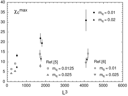
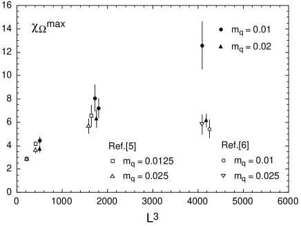
Figure 7: (a) Peak height of pseudo chiral susceptibility $\chi_{c}$ as a function of $m_{q}$ for various spatial volumes. (b) Same for the Polyakov susceptibility $\chi_{\Omega}$. Previous results are plotted with open symbols.

We also calculate the pseudo chiral susceptibility in the present work. In Fig. 7 (a) previous data for this quantity from Refs. [7, 8] are compared with the new results. A similar comparison for the Polyakov loop susceptibility is made in Fig. 7 (b). We observe that the data are consistent for the sizes $L=8$ and $L=12$. A reasonable agreement is also seen between the present simulation and the earlier results for $L=16$ at $m_{q}=0.025-0.02$. At the smallest quark mass of $m_{q}=0.01$, however, the result from Ref. [8] is by a factor $2-3$ smaller compared to our values.

A technical point to note in the calculation of Ref. [8] for $\chi_{c}$ is that it used a multiple set of noise vectors for each configuration in contrast to a single vector employed in Ref. [7] and the present work. This, however, would not be the main source of the discrepancy since the result of Ref. [8] for $m_{q}=0.025$ is in agreement with the other calculations. This difference also cannot explain the discrepancy in the Polyakov susceptibility. We think it likely that the underestimate of Ref. [8] originates from a shorter length of their run. Indeed dividing our full set of trajectories at $m_{q}=0.01$ and $L=16$ into subsets of 2500 each, we find susceptibilities reduced by a similar factor for some of the subsets owing to a long-range fluctuations over $\tau\sim O(1000)$.

4 Analysis of quark mass dependence

4.1 Scaling laws and exponents

We have seen in the previous section that our finite-size data do not show clear evidence for a first order phase transition down to $m_{q}=0.01$. In the present section we assume that the two-flavor chiral transition is of second-order which takes place at $m_{q}=0$, and turns into a smooth crossover for $m_{q}\neq 0$. Various scaling laws follow from this assumption for the quark mass dependence of the susceptibilities. We analyze to what extent our data support the expected scaling laws. In particular, we examine whether the scaling exponents agree with the O(4) values as predicted by the effective sigma model analysis[3], or at least the O(2) values corresponding to exact $U(1)$ chiral symmetry of the Kogut-Susskind quark action used in our simulations.

The scaling laws follow from a well-known renormalization-group argument which predicts that the leading singularity of the free energy per unit volume has the scaling form

$$f_{s}(t,h)=h^{d/y_{h}}\phi(t\cdot h^{-y_{t}/y_{h}}),$$ (30)

where $t$ and $h$ are reduced temperature and quark mass, $y_{t}$ and $y_{h}$ are the thermal and magnetic critical exponents, and $d=3$ is the space dimension. We take the reduced variables to be

$$t = \beta_{c}(m_{q})-\beta_{c}(0),$$ (31)

$$h = m_{q},$$ (32)

where $\beta_{c}(m_{q})=6/g_{c}^{2}(m_{q})$ denotes the pseudo critical coupling defined as the peak position of a susceptibility for a given quark mass $m_{q}$. The choice for $h$ corresponds to $h\propto m_{q}/T$ up to a numerical factor of 4. The scaling law for the pseudo critical coupling is then given by

$$\beta_{c}(m_{q})=\beta_{c}(0)+c_{g}m_{q}^{z_{g}}$$ (33)

with

$$z_{g}=\frac{y_{t}}{y_{h}}.$$ (34)

One can define three types of susceptibilities depending on the combination of variables taken for the second derivative of the free energy. The $(h,h)$ combination corresponds to the chiral susceptibility $\chi_{m}$, and we find the scaling form of its peak height to be

$$\chi_{m}^{max}(m_{q})=c_{m}m_{q}^{-z_{m}},$$ (35)

where

$$z_{m}=2-\frac{d}{y_{h}}.$$ (36)

The $t$ derivative generates susceptibilities involving the energy operator $\epsilon$. Decomposing $\epsilon$ into the gluon terms that depend on the spatial and temporal plaquette averages and the quark term proportional to $\overline{\psi}D_{0}\psi$, we expect

$$\chi_{t,i}^{max}(m_{q}) = c_{t,i}\ m_{q}^{-z_{t,i}},\qquad i=f,\sigma,\tau,$$ (37)

$$\chi_{e,i}^{max}(m_{q}) = c_{e,i}\ m_{q}^{-z_{e,i}},\qquad i=f,\sigma,\tau,$$ (38)

$$\chi_{e,ij}^{max}(m_{q}) = c_{e,ij}\ m_{q}^{-z_{e,ij}},\qquad i,j=\sigma,\tau$$ (39)

For these susceptibilities only the leading exponent needs to be constrained by the thermal and magnetic exponents, i.e.,

$$z_{t} = 1+\frac{y_{t}}{y_{h}}-\frac{d}{y_{h}},\qquad z_{t}=\mbox{max}_{i=f,\sigma,\tau}\{z_{t,i}\},$$ (40)

$$z_{e} = \frac{2y_{t}}{y_{h}}-\frac{d}{y_{h}},\qquad z_{e}=\mbox{max}_{i=f,\sigma,\tau,j,k=\sigma,\tau}\{z_{e,i},z_{e,jk}\}.$$ (41)

Since all the exponents are expressed in terms of $y_{t}$ and $y_{h}$, two relations exist among the four exponents $z_{g},z_{m},z_{t}$ and $z_{e}$, which may be taken to be

$$z_{g}+z_{m} = z_{t}+1,$$ (42)

$$2z_{t}-z_{m} = z_{e}.$$ (43)

4.2 Results for exponents

Our study of exponents is based on the results for the peak position and height of various susceptibilities summarized in Table 2. For $m_{q}=0.01$ and $L=12$ two runs are made. We present results employing the first run carried out at $\beta=5.266$, since the exponents obtained with the second run are consistent with those with the first run.

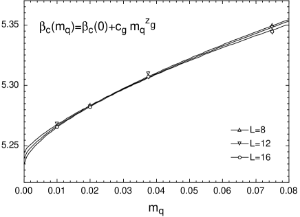
Figure 8: Pseudo critical coupling $\beta_{c}(m_{q})$ as a function of $m_{q}$ determined from the peak position of susceptibility $\chi_{m}$. Lines are fits to (33).

Let us start with an examination of the exponent $z_{g}$ that governs the scaling behavior of the critical coupling $\beta_{c}(m_{q})$. In Fig. 8 we plot $\beta_{c}(m_{q})$ defined as the peak position of the chiral susceptibility $\chi_{m}$. Solid lines represent fit of the data to the form (33), which reasonably go through the data points. Results for $z_{g}$ are listed in the first row of Table 3. Other susceptibilities yield results consistent with those from $\chi_{m}$ well within the errors.

We observe that the values of $z_{g}$ do not exhibit clear size dependence, and are in agreement with the theoretical predictions based on O(2) or O(4) symmetry within one to two standard deviations. As expected from this observation, a reasonable fit is also obtained fixing $z_{g}$ to either the O(2) or O(4) exponent.

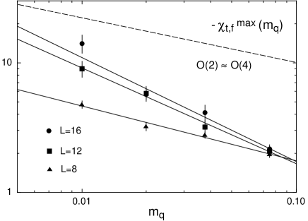
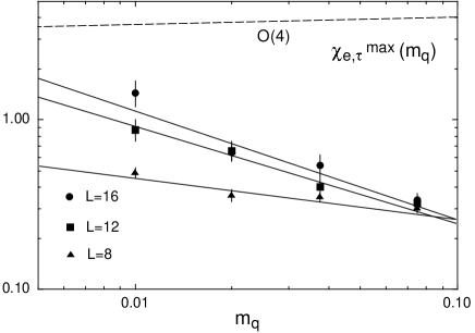
Figure 9: Peak height of susceptibility $\chi_{m}$, $\chi_{t,f}$ and $\chi_{e,\tau}$ as a function of $m_{q}$ for fixed spatial size $L$. Lines are fits to a single power $\chi_{i}\propto m^{-z_{i}}$. Dashed lines indicate slope expected for O(2) or O(4) exponents.

Let us turn to the exponents determined from peak height of the susceptibilities. In Fig. 9 we plot the quark mass dependence of peak height for the representative susceptibilities. Exponents are extracted by fits employing a scaling behavior with a single power as given in (35, 37-39). Results are summarized in Table 3. For $z_{t}$ and $z_{e}$ various operator combinations yield results which are in mutual agreement within estimated errors.

Table 3: Critical exponents extracted by fits of critical coupling and peak height of susceptibilities for fixed spatial size $L$ as compared to $O(2),O(4)$[21, 22, 23] and mean-field (MF) values.

	O(2)	O(4)	MF	$L=8$	$L=12$	$L=16$
$z_{g}$	0.60	0.54	2/3	0.70(11)	0.74(6)	0.64(5)
$z_{m}$	0.79	0.79	2/3	0.70(4)	0.99(8)	1.03(9)
$z_{t}$	0.39	0.33	1/3
$z_{t,f}$				0.42(5)	0.75(9)	0.78(10)
$z_{t,\sigma}$				0.47(5)	0.81(10)	0.82(12)
$z_{t,\tau}$				0.47(5)	0.81(9)	0.83(12)
$z_{e}$	-0.01	-0.13	0
$z_{e,f}$				0.21(4)	0.28(7)	0.38(7)
$z_{e,\sigma}$				0.25(6)	0.56(11)	0.58(13)
$z_{e,\tau}$				0.22(6)	0.52(10)	0.55(12)
$z_{e,\sigma\sigma}$				0.18(5)	0.46(8)	0.43(10)
$z_{e,\sigma\tau}$				0.20(5)	0.51(9)	0.50(12)
$z_{e,\tau\tau}$				0.19(5)	0.48(9)	0.47(11)

We observe that all the exponents $z_{m},z_{t}$ and $z_{e}$ exhibit a sizable increase between $L=8$ and 12, and the larger values stay for $L=16$. Comparing the exponents with those of O(2), O(4) or mean-field (MF) predictions, we find that an apparent agreement of $z_{m}$ and $z_{t}$ for the smallest size $L=8$ becomes lost for $L\geq 12$. The magnitude of discrepancy is smallest for $z_{m}$, for which we find a 10–20% larger value amounting to a one to two standard deviation difference. For $z_{t}$ the discrepancy is by a factor two for $L=12$ and 16. The disagreement is even more pronounced for the exponent $z_{e}$ for which a value in the range $z_{e}\approx 0.5-0.6$ is obtained in contrast to negative values for O(2) and O(4).

One can ask how inclusion of subleading singularities and/or analytic terms in the fitting function modifies the results above. A thorough examination of this question is difficult with our limited data sets, and we restrict ourselves to the simplest case where a constant term is included in the fit: $\chi_{i}^{max}(m_{q})=c_{i0}+c_{i1}m_{q}^{-z_{i}}$. The points to be examined are (i) how the values of exponents change, and (ii) whether reasonable fits are obtained with the exponents fixed to theoretically expected values.

Concerning (i), the fitted values of $z_{m}$ and $z_{t}$ for $L=8$ and 12 are consistent with the results of single-power fits, while those for $L=16$ become larger and take a value $z\approx 1.5\pm 0.5$. For $z_{e}$ large values of such a magnitude are obtained for all three sizes $L=8$, 12 and 16 with similar errors. Thus adding a constant term does not alleviate the discrepancy.

Turning to (ii), the quality of fit significantly worsens when one fixes the value of exponents to the theoretical value. Values of $\chi^{2}$ per degree of freedom increase to $2-3$ as compared to $0.5-1$ for the single-power fit with $z_{i}$ as a free parameter, and the fit generally misses the point for the smallest quark mass $m_{q}=0.01$ for $L=16$. In particular the fit for $\chi_{e}$ accommodates a negative value of $z_{e}$ only by forcing the coefficient $c_{e,1}$ in front of the power term to a negative value of a magnitude similar to that of the constant term $c_{e,0}$. Altogether fits with theoretical values of exponents do not appear any more reasonable than fits with a single power.

These examinations lead us to conclude that the exponents do show a trend of deviation from the O(2) or O(4) values, at least in the range of quark mass $m_{q}=0.075-0.01$ explored in our simulation.

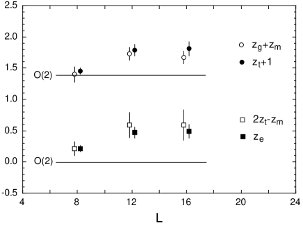
Figure 10: Consistency check of exponents for a given spatial size $L$. Horizontal lines indicate values expected for O(2) exponents. Values for O(4) are similar.

Let us recall from Sec. 4.1 that the four exponents $z_{g}$, $z_{m}$, $z_{t}$ and $z_{e}$ should satisfy two consistency equations (42–43). In Fig. 10 we plot the two sides of the hyperscaling equations using the exponents obtained with a single power fit in Table 3. For $z_{t}$ and $z_{e}$ we take averages over the channels as the exponents are mutually consistent. We observe that the hyperscaling relations are well satisfied for each spatial volume even though the values of individual exponents change from volume to volume and deviate from theoretical expectations. This implies that our susceptibility data are consistent with a second-order transition at $m_{q}=0$ governed by the magnetic and thermal operators.

Given this result, we may estimate the magnetic and thermal exponents through a $\chi^{2}$ fit of the four exponents $z_{g,m,t,e}$ to the form (34, 36, 40, 41). Using average values of results in Table 3 for $z_{t}$ and $z_{e}$, we find $(y_{h},y_{t})=(2.31(7),1.74(5))(L=8)$, $(3.02(19),2.24(12))(L=12)$ and $(3.31(25),2.22(15))(L=16)$, as compared to $(2.48,1.49)$ for O(2) symmetry and $(2.49,1.34)$ for O(4) symmetry[21, 22, 23].

4.3 Results for scaling function

Defining a scaling variable

$$x=\left(\beta_{c}(m_{q})-\beta_{c}(0)\right)\cdot m_{q}^{-z_{g}},$$ (44)

one expects the singular part of the susceptibility to take the functional form

$$\chi_{m}(\beta,m_{q})=m_{q}^{-z_{m}}\cdot F_{m}(x).$$ (45)

Figure 11: Scaling function $F_{m}(x)$ calculated by $\chi_{m}(\beta,m_{q})\cdot(m_{q}/0.01)^{z_{m}}$ as a function of $x=\left(\beta_{c}(m_{q})-\beta_{c}(0)\right)\cdot(m_{q}/0.01)^{-z_{g}}$for $L=16$ using (a) measured values $z_{g}=0.6447,z_{m}=1.033,\beta_{c}(0)=5.2353$, and (b) O(4) values $z_{g}=0.538$ and $z_{m}=0.794$ and measured value $\beta_{c}(0)=5.2253$.

We plot in Fig. 11 two estimates of the scaling function $F_{m}(x)$ calculated as $\chi_{m}(\beta,m_{q})\cdot(m_{q}/0.01)^{z_{m}}$ using data for $L=16$: in (a) we employ the measured values $z_{g}=0.6447$, $z_{m}=1.033$, $\beta_{c}(0)=5.2353$, and in (b) we take the O(4) values[23] for the exponents $z_{g}=0.538$, $z_{m}=0.794$ and substitute the value $\beta_{c}(0)=5.2253$ obtained with a fit of $\beta_{c}(m_{q})$ with $z_{g}$ fixed to the O(4) value. Similar to the experience with fits of peak height in Sec. 4.2, we find that scaling is reasonable with the use of the measured exponents. The fit, however, worsens if the O(4) exponents are employed; in particular the curve for the smallest quark mass $m_{q}=0.01$ deviates largely from the rest.

5 Conclusions

In this article we have presented results of our analysis of the two-flavor chiral phase transition with the Kogut-Susskind quark action on an $N_{t}=4$ lattice. By studying the spatial volume dependence of various susceptibilities, we have confirmed the conclusion of previous investigations[7, 8] that the transition is a smooth crossover for $m_{q}\geq 0.02$. At $m_{q}=0.01$ the susceptibilities exhibit an almost linear increase in spatial volume between $8^{3}$ and $16^{3}$ lattices, which contradicts the results of previous work[8], and may appear to be consistent with a first-order phase transition. However, examination of time histories and histograms of observables, and in particular, a rescaling of spatial size in terms of the zero-temperature pion mass strongly suggests that the linear increase is a transient phenomenon arising from an insufficient spatial size. It is our present conclusion that there is no evidence indicating a first order transition down to $m_{q}=0.01$.

We have also analyzed how susceptibilities depend on the quark mass. The pattern of critical exponents we have obtained is consistent with the existence of a second-order phase transition at $m_{q}=0$, which is governed by a renormalization-group fixed point with two relevant operators, the energy and magnetization operators. The exponents, however, do not agree with O(2), O(4) or mean-field theory predictions. This means that the theoretical argument for a second order phase transition from the chiral sigma model remains unjustified in the present work.

A disagreement with the O(4) values may not come as a surprise since flavor symmetry breaking effects of the Kogut-Susskind quark action is quite large at $\beta\approx 5.3$ where the transition is located for $N_{t}=4$. Indeed masses of non-Nambu-Goldstone pions are closer to those of $\rho$ meson, rather than those of the Nambu-Goldstone pion, for these values of $\beta$.

Numerically, the O(2) values for exponents are close to those for O(4). The deviation from the O(2) values is theoretically more puzzling for several reasons: (i) O(2) is an exact symmetry group of the Kogut-Susskind action for any lattice spacing, (ii) this symmetry is preserved under the algorithmic expedient of taking a square root of the quark determinant adopted in the hybrid R algorithm, and (iii) the susceptibility $\chi_{m}$ is precisely the second derivative of free energy with respect to the quark mass which is the conjugate field of the O(2) order parameter. Thus, if the two-flavor system simulated by the hybrid R algorithm undergoes a second-order transition, we expect the O(2) values of exponents to emerge toward the chiral limit.

The smallest quark mass $m_{q}=0.01$ we have explored is quite small at $\beta\approx 5.3$, corresponding to $m_{\pi}/m_{\rho}\approx 0.19$ which is close to the experimental value of 0.18. It is possible, however, that the critical region where susceptibilities exhibit the true scaling behavior is located even nearer to the chiral limit. If this is the origin of the discrepancy, establishing the universality nature of the two-flavor transition for the Kogut-Susskind quark action will require further simulations toward substantially smaller quark masses and necessarily much larger spatial lattices.

References

- [1]
- [2]
- [3] R. D. Pisarski and F. Wilczek, Phys. Rev. D29 (1984) 338; F. Wilczek, Int. J. Mod. Phys. A7 (1992) 3911; K. Rajagopal and F. Wilczek, Nucl. Phys. B399 (1993) 395.
- [4] For reviews and references on the issue of the order of chiral transition, see, M. Fukugita, Nucl. Phys. B (Proc. Suppl.) 4 (1988) 105; Lattice 88, Nucl. Phys. B (Proc. Suppl.) 9 (1989) 291; A. Ukawa, Lattice 89, Nucl. Phys. B (Proc. Suppl.) 17 (1990) 118; S. Gottlieb, Lattice 90, Nucl. Phys. B (Proc. Suppl.) 20 (1991) 247; D. Toussaint, Lattice 91, Nucl. Phys. B (Proc. Suppl.) 26 (1992) 3.
- [5] Collaboration, R. V. Gavai et al., Phys. Lett. B232 (1989) 491; ibid. B241 (1990) 567.
- [6] F. R. Brown, F. P. Butler, H. Chen, N. H. Christ, Z. Dong, W. Schaffer, L. I. Unger and A. Vaccarino, Phys. Lett. B251 (1990) 181.
- [7] M. Fukugita, H. Mino, M. Okawa and A. Ukawa, Phys. Rev. Lett. 65 (1990) 816; Phys. Rev. D42 (1990) 2936.
- [8] F. R. Brown, F. P. Butler, H. Chen, N. H. Christ, Z. Dong, W. Schaffer, L. I. Unger and A. Vaccarino, Phys. Rev. Lett. 65 (1990) 2491; A. Vaccarino, Lattice 90, Nucl. Phys. B (Proc. Suppl.) 20 (1991) 263.
- [9] F. Karsch, Phys. Rev. D49 (1994) 3791.
- [10] F. Karsch and E. Laermann, Phys. Rev. D50 (1994) 6954.
- [11] A. Ukawa, Lattice 96, Nucl. Phys. B (Proc. Suppl.) 53 (1997) 106; JLQCD Collaboration (S. Aoki et al.), talk presented by M. Okawa at the International Workshop “Lattice QCD on Parallel Computers” (Tsukuba, March 10-15, 1997), to be published in the proceedings, KEK-CP-062 (hep-lat/9708010).
- [12] G. Boyd, F. Karsch, E. Laermann and M. Oevers, BI-TP 96/27 (hep-lat/9607046); E. Laermann, talk presented at the International Workshop “Lattice QCD on Parallel Computers” (Tsukuba, March 10-15, 1997), to be published in the proceedings; E. Laermann, plenary talk presented at Lattice’97, to be published in the proceedings.
- [13] D. Toussaint, talk presented at the International Workshop “Lattice QCD on Parallel Computers” (Tsukuba, March 10-15, 1997), to be published in the proceedings; C. DeTar, poster presented at Lattice’97, to be published in the proceedings.
- [14] S. Gottlieb, W. Liu, D. Toussaint, R. L. Renken and R. L. Sugar, Phys. Rev. D35 (1987) 2531.
- [15] Y. Kuramashi, M. Fukugita, H. Mino, M. Okawa and A. Ukawa, Phys. Rev. Lett. 71 (1993) 2387 ; ibid. 72 (1994) 3448.
- [16] I. R. McDonald and K. Singer, Discuss. Faraday Soc. 43 (1967) 40; A. M. Ferrenberg and R. H. Swendsen, Phys. Rev. Lett. 61 (1988) 2635; ibid. 63 (1989) 1195.
- [17] Z. Dong and N. H. Christ, Lattice 91, Nucl. Phys. B (Proc. Suppl.) 26 (1992) 314.
- [18] T. Blum, L. Kärkkäinen, D. Toussaint and S. Gottlieb, Phys. Rev. D51 (1995) 5153.
- [19] M. Fukugita, M. Okawa and A. Ukawa, Nucl. Phys. B337 (1990) 181.
- [20] M. Fukugita, H. Mino, M. Okawa and A. Ukawa, J. Phys. A: Math. Gen. 23 (1990) L561.
- [21] G. A. Baker, B. G. Nickel and D. I. Meiron, Phys. Rev. B17 (1978) 1365.
- [22] J. C. Le Guillou and J. Zinn-Justin, Phys. Rev. B21 (1980) 3976; J. Phys. Lett. (Paris) 46 (1985) L137.
- [23] K. Kanaya and S. Kaya, Phys. Rev. D51 (1995) 2404.