Monopole Percolation in the Compact Abelian Higgs Model

Abstract

We have studied the monopole-percolation phenomenon in the four dimensional Abelian theory that contains compact $U(1)$ gauge fields coupled to unitary norm Higgs fields. We have determined the location of the percolation transition line in the plane $(\beta_{g},\beta_{H})$. This line overlaps the confined-Coulomb and the confined-Higgs phase transition lines, originated by a monopole-condensation mechanism, but continues away from the end-point where this phase transition line stops. In addition, we have determined the critical exponents of the monopole percolation transition away from the phase transition lines. We have performed the finite size scaling in terms of the monopole density instead of the coupling, because the density seems to be the natural parameter when dealing with percolation phenomena.

I Introduction

Much work has been devoted in recent years to the understanding of the pure gauge $U(1)$ lattice field theory. Despite the apparent simplicity of this model, which can be considered a limit of the well known $Z(n)$ gauge models in four dimensions, the order of their phase transition is a rather controversial issue. Pioneering simulations suggested that the transition was actually of second order, i.e., a continuum limit for this lattice theory is possible [1]. Posterior analysis showed the presence of a two-peak structure in the histograms questioning the order of the phase transition [2, 3]. Several new approaches have been proposed: extended lattice actions [4], different topologies [5, 6], monopole suppressed actions [7], etc. For a summary of the history of this transition see Ref. [8].

The main point in order to clarify the nature of the phase transition in pure gauge $U(1)$ lattice field theory is the understanding of the role of topological excitations. This analysis was initiated in the early eighties by several groups: Einhorn and Savit [9] and Banks, Kogut and Myerson [10]. Their conclusion was that topological excitations are actually strings of monopole current. In addition, DeGrand and Toussaint [11] showed that these monopoles can be actually studied by direct numerical simulation, in particular the monopole condensation phenomenon over the phase transition. On the other hand, it is widely accepted that the observed problems in the analysis of the phase transition can be related to the one-dimensional character of the topological excitations.

An important observation was made by Kogut, Kocić and Hands [12]. They showed that in pure gauge non-compact $U(1)$ (i.e. the action obtained keeping only the first order in the Taylor expansion) which is Gaussian, monopoles percolate and satisfy the hyperscaling relations characteristic of an actual second-order phase transition.

Baig, Fort and Kogut [13] showed that in the compact pure gauge theory, just over the phase transition point, monopoles not only condensate but also percolate. They pointed out that the strange behavior of this phase transition –its unexpected first order character and strange critical exponents– can be related to the coincidence of these two phenomena.

Furthermore, Baig, Fort, Kogut and Kim [14] showed that in the case of non-compact QED coupled to scalar Higgs fields, the monopole percolation phenomena –previously observed over the gauge line– actually propagate into the full $(\beta_{g},\beta_{H})$ plane, being $\beta_{g}$ and $\beta_{H}$ the gauge and Higgs couplings.

It is surprising that the monopole percolation phenomenon is not related to the phase transition line that separates the confined and the Higgs phases, a second order transition that is logarithmically trivial.

In the present paper we have performed a numerical simulation of the compact lattice gauge $U(1)$ coupled to Higgs fields of unitary norm. First of all, we have reproduced some results concerning the phase diagram previously obtained by Alonso et al. [15], but we have measured at the same time the behavior of monopoles, condensation and percolation. We have determined the location of the percolation transition line –the line defined by the maxima of the monopole susceptibility– in the plane $(\beta_{g},\beta_{H})$. We have observed that this line overlaps the confined-Coulomb and the confined-Higgs phase transition lines, which result by a monopole-condensation mechanism. But it continues away from the end point where this phase transition line stops. In addition, we have determined the critical exponents of the monopole percolation transition away from the phase transition lines. We have performed the finite size scaling in terms of the monopole density instead of the coupling, because the density seems to be the natural parameter when dealing with percolation phenomena.

The plan of the paper is the following: In Sec. II we define our model and we analyze the appearance of the topological excitations. In Sec. III we extend the standard percolation analysis to the case of monopole percolation, using densities as critical parameters. Sec. IV A contains the result of the relation between monopole percolation and phase transition Sec. IV B is devoted to the finite size analysis of the percolation phenomena. Finally, Sec.V contains the conclusions of this work.

II The Model

A The action

In this paper, we resume the work initiated in Ref. [13], and focus on the compact abelian Higgs Model with a fixed length scalar field whose action is

$$S=-\beta_{g}\sum_{n\mu\nu}\cos\Theta_{\mu\nu}(n)-\beta_{H}\sum_{x,\mu}\left(\phi_{x}^{*}U_{x,\mu}\phi_{x+\mu}+c.c.\right),$$ (1)

where $\Theta_{\mu\nu}(n)$ is the circulation of the compact gauge field around a plaquette, $\beta_{g}=1/e^{2}$ is the gauge coupling and $\phi_{x}=\exp{i\alpha(x)}$ is a phase factor. We choose fixed length Higgs fields because it has been shown that they live in the same universality class than conventional variable length Higgs fields but have the advantage that they do not require fine-tuning [17]. In addition, we want to keep as close as possible to the analysis of the non-compact Abelian Higgs Model of Refs. [14, 18] in order to compare to non-compact scalar electrodynamics, whose action is

$$S_{nc}=\frac{1}{2}\beta_{g}\sum_{n\mu\nu}\Theta_{\mu\nu}(n)^{2}-\beta_{H}\sum_{x,\mu}\left(\phi_{x}^{*}U_{x,\mu}\phi_{x+\mu}+c.c.\right).$$ (2)

The phase diagrams for the two models are well known. They are qualitatively represented in Fig. 1. Non-compact scalar QED has two disconnected phases: a Coulomb phase and a Higgs phase. It is important to remark that there is not phase transition over the pure gauge axis. In contrast, in the compact case a transition separates the Coulomb and the confined phase while the transition separating the confined and Higgs phases has an end point (point $E$ in the Fig. 1a).

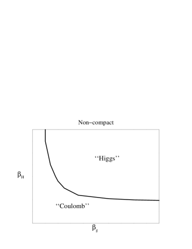
(a) (b)

FIG. 1.: Qualitative phase diagrams for the compact and non-compact scalar QED.

B Monopoles

Following [11] we can separate the plaquette angle $\Theta_{\mu\nu}$ into two pieces: physical fluctuations which lie in the range $-\pi$ to $\pi$ and Dirac strings which carry $2\pi$ units of flux. Introducing an electric charge $e$ we define an integer-valued Dirac string by

$$e\Theta_{\mu\nu}=e\bar{\Theta}_{\mu\nu}(\tilde{n})+2\pi S_{\mu\nu},$$ (3)

where the integer $S_{\mu\nu}$ determines the strength of the string threading the plaquette and $e\Theta_{\mu\nu}$ represents physical fluctuations. The integer-valued monopole current, $m_{\mu}(n)$, defined on links of the dual lattice, is then

$$m_{\mu}(\tilde{n})={1\over 2}\epsilon_{\mu\nu\kappa\lambda}\Delta_{\nu}^{+}S_{\kappa\lambda}(n+\hat{\mu}),$$ (4)

where $\Delta_{\nu}^{+}$ is the forward lattice difference operator, and $m_{\mu}$ is the oriented sum of the $S_{\mu\nu}$ around the faces of an elementary cube. This gauge-invariant definition implies the conservation law $\Delta_{\mu}^{-}m_{\mu}(\tilde{n})=0$, which means that monopole world lines form closed loops.

The appearance of topological excitations in the abelian Higgs model was studied in Ref. [9, 10]. Furthermore, in Ref [19] a Monte Carlo simulation was performed to look for the density of monopoles. They observed that the confined (Higgs and Colulomb) phase was characterized by a large (vanishing) density of monopoles vortices and electric current densities.

III Percolation

A Concepts of percolation

The role of the monopole percolation in this model is analyzed using the techniques of standard percolation [20]. In the simplest models the sites are occupied with a probability $p$. One can define a cluster as a group of occupied sites connected by nearest-neighbor distances. When a cluster becomes infinite in extent, it is called a percolation cluster. Obviously, for $p=0$ all the sites are empty and there is no percolation cluster. For $p=1$ all the sites are occupied and one percolation cluster exists. There exists a critical concentration $p_{c}$ such that for $p<p_{c}$ ($p>p_{c}$) no (one) percolation cluster exists. This is the typical behavior of a phase transition. We define $P_{\infty}$ as the probability for an occupied site to belong to the infinite cluster.

If we define $g_{n}$ as the relative number of clusters of size $n$, the probability of any site to belong to a cluster of size $n$ is $ng_{n}$. According to this definitions, the mean cluster size is

$$S=\frac{\sum_{n}n^{2}g_{n}}{\sum_{n}ng_{n}},$$ (5)

where the infinite cluster is excluded from the sum. This quantity diverges at the critical concentration.

Thus, $P_{\infty}$ is the order parameter of the transition and $S$ is its associated susceptibility. Their behaviors near the critical point are:

$$P_{\infty}\sim\left(p-p_{c}\right)^{\beta}\\ \hskip 28.45274pt\mathrm{for}\hskip 12.0ptp>p_{c},$$ (6)

and

$$S\sim\left|p-p_{c}\right|^{-\gamma}.$$ (7)

B Percolation of monopoles in QED

We have defined the monopole current $m_{\mu}(x)$ in eq. (4). One can define a connected cluster of monopoles as a set of sites joined by monopole line elements [21]. Notice that this definition ignores the fact that monopoles are actually vectors. The density of occupation is

$$\rho=\frac{n_{tot}}{L^{4}}=\sum_{n=4}^{n_{max}}g_{n}n,$$ (8)

where $n_{tot}$ is the total number of connected sites and $n_{max}$ is the size of the largest cluster. The number 4 in the sum comes from the conservation law.

The order parameter ($P_{\infty}$) is

$$M=\frac{n_{max}}{n_{tot}}.$$ (9)

Its corresponding susceptibility (the mean cluster size $S$) is

$$\chi=\frac{1}{n_{tot}}\left(\sum_{n=4}^{n_{max}}g_{n}n^{2}-n^{2}_{max}\right).$$ (10)

Near the critical point, $M$ should have a non analytical behavior with a “magnetic” exponent $\beta$. We have followed lines of constant $\beta_{H}$, so

$$M\sim\left(\beta_{g}^{c}-\beta_{g}\right)^{\beta}\hskip 28.45274pt\mathrm{for}\hskip 12.0pt\beta_{g}<\beta_{g}^{c}.$$ (11)

where the upperscript $c$ means “critical”. The susceptibility also diverges:

$$\chi\sim\left(\beta_{g}^{c}-\beta_{g}\right)^{-\gamma}.$$ (12)

One should remark that the natural parameter when studying percolation is the probability of occupation (in random percolation it determines all the observables). In a lattice gauge model, the fundamental variables are the couplings, which determine all the other observables. In particular, they determine the density of monopoles $\rho$, i.e., the probability of occupation. In this sense, it is also possible to parameterize percolation as a function of the densities. In this case the critical behavior will be

$$M\sim\left(\rho-\rho_{c}\right)^{\beta}\hskip 28.45274pt\mathrm{for}\hskip 12.0pt\beta_{g}<\beta_{g}^{c},$$ (13)

and

$$\chi\sim\left(\rho-\rho_{c}\right)^{-\gamma}.$$ (14)

Clearly, the two parameterizations might have the same critical exponents, but the first one seems to exhibit stronger finite size effects.

IV Numerical results

A Phase transition vs. monopole percolation

We have performed numerical simulations with the action (1) on hypercubical lattices with standard periodic boundary conditions. In these simulations we have measured the internal gauge and Higgs energies

$$E_{g}=\sum_{n\mu\nu}\cos\Theta_{\mu\nu}(n),$$ (15)

$$E_{H}=\sum_{x,\mu}\left(\phi_{x}^{*}U_{x,\mu}\phi_{x+\mu}+c.c.\right).$$ (16)

as well as all magnitudes related to monopole percolation, i.e. $\rho$, $M$ and $\chi$, which are defined in eqs. (8, 9, 10) respectively.

In order to locate the continuation into the full $(\beta_{g},\beta_{H})$ plane of the monopole percolation transition previously determined over the pure gauge axis in Ref [13], we have performed repeated measurements over thermal cycles changing the $\beta_{g}$ coupling, until the entire region inside the limits $0<\beta_{g}<1.5$ and $0<\beta_{H}<1.5$ has been covered. In particular, the confined-Coulomb and confined-Higgs phase transition lines. Lattice size for this exploratory runs has been of $6^{4}$ and the $\beta_{g}$ step has been $\Delta\beta_{g}=0.005$.

We have not used any reweighting technique when measuring the monopole-related magnitudes. In all the plots, lines are only to guide the eyes and the errors are not shown because they are smaller than the symbols used.

The number of iterations at each $\beta_{g}$ value has been $30.000$, discarding the first $10.000$. In addition, several thermal cycles have been performed at different values of $\beta_{H}$ in order to determine the location of the Coulomb-Higgs phase transition line.

Fig. 2 collects the results of these runs. The small black points represent the maximum of the monopole susceptibility. The solid line is the phase-transition line. Note that the monopole percolation transition line is on top of both the confined-Coulomb line and the confined-Higgs line up to the end point. Beyond this point monopole percolation transition line continues, now unrelated to any energy phase transition, approaching the vertical axis. This behavior is in clear contrast with the non-compact case [14] where the monopole-transition is completely independent of the Coulomb-Higgs phase transition.

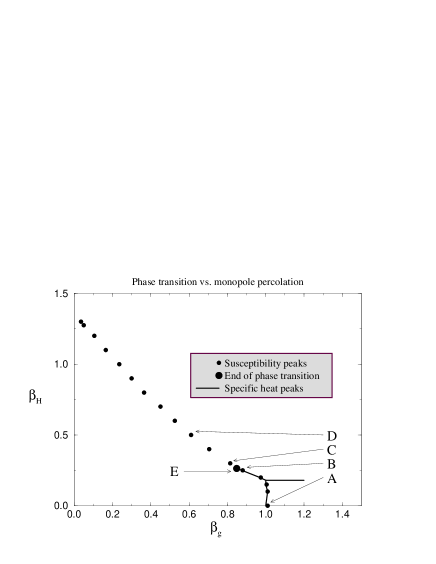
FIG. 2.: The plane $(\beta_{g},\beta_{H})$ showing the lines of phase transition and the monopole percolation. Thermal cycles have been done at fixed $\beta_{H}$ values: A ($\beta_{H}=0.00$), B ($\beta_{H}=0.25$), C ($\beta_{H}=0.30$) and D ($\beta_{H}=0.30$). The magnitudes measured along this lines are shown in the Figs. 4a, 4b, 4c and 4d respectively. The point E is the end of the phase transition.

In Fig. 3 we compare two sets of histograms corresponding to cycles: (a) for $\beta_{H}=0.25$, over the confined-Higgs phase transition line and (b) for $\beta_{H}=0.3$, i.e. just beyond the end-point $E$. In the two figures the solid line corresponds to the value of $\beta_{g}$ for which the monopole susceptibility has a maximum. The appearance of a two-peak structure over the phase transition confirms that the lattice size, the statistics used and the coupling step in the thermal cycle are enough to establish the appearance of the phase transition.

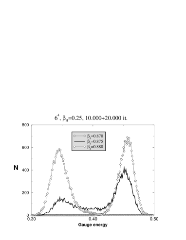
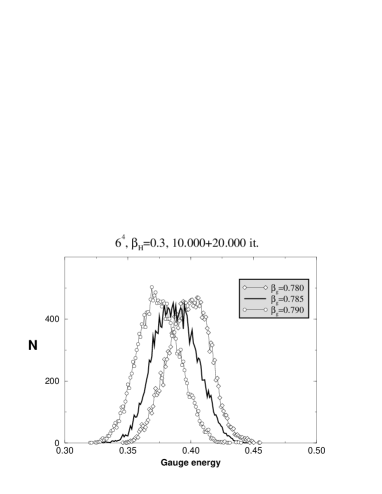
(a) (b)

FIG. 3.: Some histograms. The plot (a) is evaluated in the point $B$. Notice the clear two peaks structure revealing a first order phase transition. This structure is not present in the plot (b), evaluated in the point $C$ where no specific heat peak is present.

An interesting question to establish is the concordance of all the phenomena (phase transition, monopole condensation and monopole percolation) at the same coupling. In this sense it was proposed in Ref. [13] to use $M$ as an order parameter to determine the location of the phase transition. The existence of an end-point for the confined-Higgs phase transition line gives us a chance to check the behavior of these three parameters over and right beyond the end-point. In Fig. 4 we have collected the results for thermal cycles at different values of $\beta_{H}$. Fig. 4a corresponds to the pure gauge compact action (point $A$ in the phase diagram), the case of Ref. [13]. Fig. 4b corresponds to $\beta_{H}=0.25$, i.e., over the confined-Higgs phase transition (point $B$). The behavior of all three parameters is similar to that observed in the pure gauge case, although the discontinuity is more abrupt. Fig. 4c corresponds to $\beta_{H}=0.30$ (point $C$), just after the end point, and Fig. 4d to $\beta_{H}=0.5$ (point $D$), a line that crosses the maximum of the monopole susceptibility but is far away from the end-point. In these last cases the energy clearly shows no discontinuity and the monopole density is completely smooth. Nevertheless, the $M$ parameter shows a fast decrease corresponding to the percolation phenomena investigated in the next subsection.

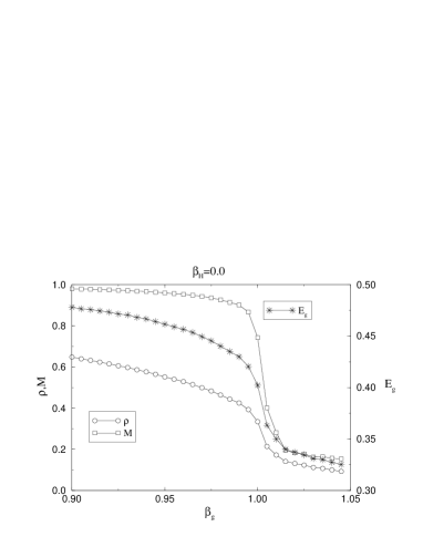
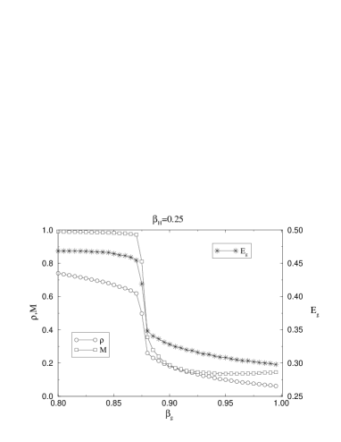
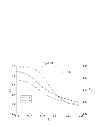
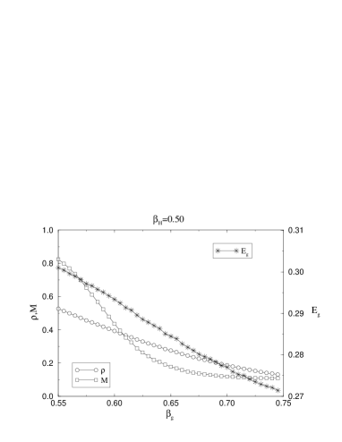
(a) (b) (c) (d)

FIG. 4.: Results for thermal cycles at different $\beta_{H}$ (points A, B, C and D in the Fig. 2). The values of $\rho$ and $M$ can be read in the left $Y$ axes, and the energies in the right $Y$ axes.

Fig. 5 shows another hint of the change of nature of the percolation at the end-point. We show the maximum of $\chi$ along the percolation line. A clear change can be seen at the end point.

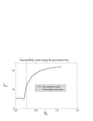
FIG. 5.: Susceptibility peaks along the percolation line. Notice the change of behavior at the end of the phase transition.

B Finite size scaling of monopole percolation transition

We want to determine the critical exponents of the monopole percolation away from the phase transition lines, at the point $D=(0.5,0.606)$ in the plane $(\beta_{g},\beta_{H})$. To do this, we keep $\beta_{H}=0.5$ fixed, and we vary $\beta_{g}$ within the range $[0.594,0.620]$ for lattice sizes ranging from $8^{4}$ to $12^{4}$. We have recorded some percolation parameters for each simulation: the density of monopoles $\rho$, $M$ and $\chi$. The statistics for each point is of $10.000$ iterations once the first $5.000$ have been discarded.

In Fig. 6, we collect the results for $M$ and $\chi$ as a function of $\beta_{g}$.

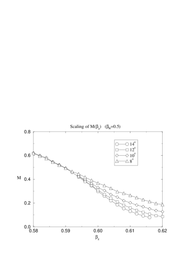
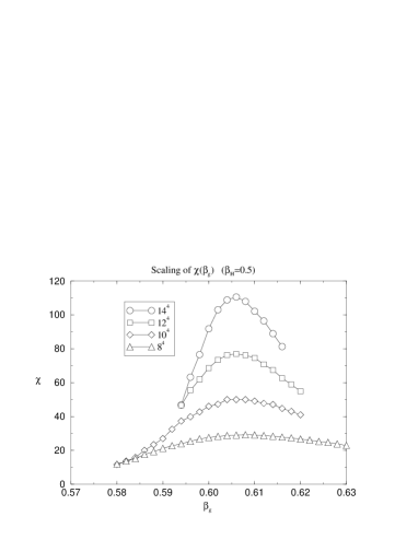
(a) (b)

FIG. 6.: $M$ (in a) and $\chi$ (in b). Both as a function of $\beta_{g}$, keeping $\beta_{H}=0.5$. The finite size effects of $M$ are stronger than in Fig. 7a.

In Fig. 7, we show the same results for $M$ and $\chi$ as a function of $\rho$.

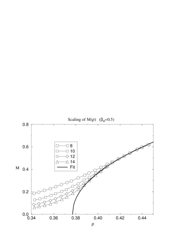
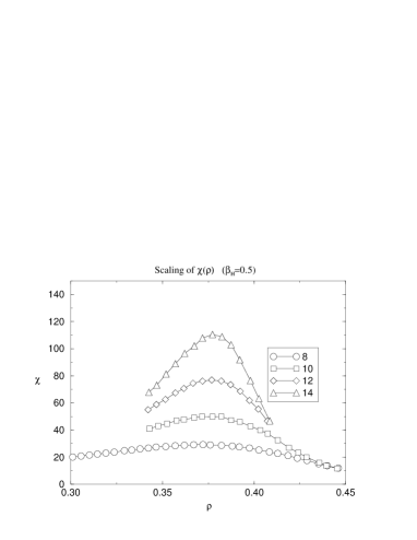
(a) (b)

FIG. 7.: $M$ (in a) and $\chi$ (in b). Both as a function of $\rho$, keeping $\beta_{H}=0.5$. The finite size effects of $M$ are lesser than in Fig. 6a.

According to finite size scaling arguments [22], the peak of the susceptibility should grow with the lattice size $L$ as

$$\chi_{max}\sim L^{\gamma/\nu},$$ (17)

and the value of $M$ at the critical point must vanish as

$$M_{crit}\sim L^{-\beta/\nu}.$$ (18)

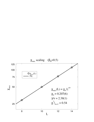
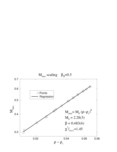
(a) (b)

FIG. 8.: Log-log plots for $\chi_{max}(L)$ and $M(\rho-\rho_{c})$, being $\rho_{c}=0.377$.

We show the value of $\chi_{max}$ as a function of $L$ in a log-log plot in the Fig. 8a. Notice that the scaling law is satisfied. A fit to eq. (17) gives

$$\frac{\gamma}{\nu}=2.38(1).$$ (19)

The straight line resulting from the fit is also shown.

We measure $\beta$ fitting the values that are not distorted by finite-size effects to the equation (13). The result is

$$\beta=0.483(4).$$ (20)

In Fig. 8b we show the selected points and the fit, with a value for the critical density about of $\rho_{c}=0.377$.

The fit of (18) is not very good. It gives $\beta/\nu=0.7(1)$. Putting our measurements of $\gamma/\nu$ into the hyperscaling relation

$$\frac{\beta}{\nu}=\frac{1}{2}\left(d-\frac{\gamma}{\nu}\right),$$ (21)

we obtain

$$\frac{\beta}{\nu}=0.81(1),$$ (22)

which is more accurate than our measurement. So, we take this value and regard the measurement as a test of hyperscaling.

Combining eqs. 20 and 22, the value of $\nu$ is

$$\nu=0.60(1).$$ (23)

The remaining critical exponents can be derived from those above using hyperscaling relations.

In the below table we compare our results with other related works:

	$p_{c}$	$\beta$	$\nu$
Our results	0.377	0.483(4)	0.60(1)
Non compact quenched QED [12]	-	0.58(2)	0.66(3)
Pure four dimensional site percolation [23]	0.161	0.715	0.683
FKL97 [16]	-	0.50(4)	0.61(4)

The vector nature of the monopole current suggests that our model do not lie in the same universality class that the four-dimensional site percolation.

We also see that our values are closed to the non-compact QED [12], but more data is required to decide if the two models belong to the same universality class.

Finally, we would like to stress the remarkable agreement with [16]. Nevertheless, they perform their analysis using a different value of the Higgs coupling, $\beta_{H}\sim 0.9$. As it pointed out in [16], a more careful analysis is necessary to decide if the critical exponents are the same along the percolation line beyond the end point.

V Conclusions

We have performed a numerical simulation of the compact lattice gauge $U(1)$ coupled to Higgs fields of unitary norm. Some results concerning the phase diagram previously obtained by Alonso et al. [15], have been confirmed but measuring at the same time the behavior of monopoles, condensation and percolation. The location of the percolation transition line –the line defined by the maxima of the monopole susceptibility– in the plane $(\beta_{g},\beta_{H})$ has been determined. This line overlaps the confined-Coulomb and the confined-Higgs phase transition lines, which are originated by a monopole-condensation mechanism, but it continues away from the end-point. This is in contrast with the behavior of the monopole percolation transition in the non-compact abelian Higgs model where it is unrelated to any phase transition. In addition, the critical exponents of the monopole percolation transition in the region far away from the phase transition lines have been determined. The finite size scaling has been performed in terms of the monopole density instead of the coupling, because the density seems to be the natural parameter when dealing with percolation phenomena.

While this paper was written up we have received Ref. [16] where a model with both, scalar and fermion matter fields has been considered. Their results for the scalar sector are in perfect agreement with our simulations. It is interesting to compare the finite size scaling analysis for the critical exponents in the pure-percolation region obtained using couplings and density parameterizations. The values obtained in both cases are in perfect agreement. However our density parameterization results have been obtained with lattice sizes smaller than those in Ref. [16]. This suggests that the finite volume effects are smaller if our parameterization is used.

- [1] B. Lautrup and M. Nauenberg Phys. Lett.95B (1980) 63.
- [2] J, Jersák, T. Neuhaus and P.M. Zerwas Phys. Lett.133B (1983) 103.
- [3] V. Azcoiti, G. Di Carlo and A.F. Grillo Phys. Lett. B267 (1991) 101.
- [4] J. Cox, W. Franzki, J. Jersák, C. B. Lang, T. Neuhaus, and P. W. Stephenson, Gauge-ball spectrum of the four-dimensional pure gauge theory, HLRZ 84/96, hep-lat/9701005, to be published in Nucl. Phys. B.
- [5] M. Baig and H. Fort Phys. Lett. B332 (1994) 428.
- [6] J. Jersák, C. B. Lang, and T. Neuhaus, Phys. Rev. D54 (1996) 6909.
- [7] B. Krishnan, U. M. Heller, V. K. Mitrjushkin, M. Mueller-Preussker, Compact U(1) Lattice Gauge-Higgs Theory with Monopole Suppression, hep-lat/9605043.
- [8] A. Bode, K. Schilling, V. Bornyakov and T. Lippert Proceedings of International RCNP Workshop on Color Confinement and Hadrons, edited by H. Toki et. al. World Scientific (1995) 247.
- [9] M. B. Einhorn and R. Savit, Phys. Rev. D17 (1978) 2583; D19 (1979) 1198.
- [10] T. Banks, R. Myerson, and J. Kogut, Nucl. Phys. B129 (1977) 493.
- [11] T. A. DeGrand and D. Toussaint Phys. Rev. D22 (1980) 2478.
- [12] A. Kocić, J.B. Kogut and S.J. Hands, Phys.Lett. B289 (1992) 400.
- [13] M. Baig, H. Fort and J.B. Kogut, Phys.Rev. D50 (1994) 5920.
- [14] M. Baig, H. Fort, J.B. Kogut and S. Kim, Phys.Rev. D51 (1995) 5216.
- [15] J.L. Alonso et al., Nucl. Phys. B405 (1993) 574.
- [16] W. Franzki, J.B. Kogut and M.P. Lombardo Chiral transition and monopole percolation in lattice scalar QED with quenched fermions, hep-lat/9707002.
- [17] D. Callaway and R. Petronzio Nucl.Phys. B277 (1986) 50.
- [18] M. Baig, E. Dagotto, J. Kogut and A. Moreo Phys. Lett. B242 (1990) 444.
- [19] J. Ranft, J. Kripfganz and G. Ranft Phys. Rev. D28 (1982) 360.
- [20] D. Stauffer, Phys. Rep. 54 (1979) 1.
- [21] S. Hands and R. Wensley, Phys. Rev. Lett. 63 (1989) 2169.
- [22] M.N. Barber in Phase transitions and critical phenomena Vol. 8, edited by C. Domb and M.S. Green, Academic Press (1983).
- [23] H.G. Ballesteros, L.A. Fernández, V. Martín-Mayor, A. Muñoz Sudupe, G. Parisi and J.J. Ruiz-Lorenzo, Measures of critical exponents in the four-dimensional site percolation, hep–lat/9612024.