1) The Influence of Gribov Copies on Gluon and Ghost Propagators in Landau Gauge and 2) A New Implementation of the Fourier Acceleration Method

Abstract

We study the influence of Gribov copies on gluon and ghost propagators in lattice Landau gauge. For the gluon propagator, Gribov noise seems to be of the order of magnitude of the numerical accuracy. On the contrary, for the ghost propagator, Gribov noise is clearly observable, at least in the strong-coupling regime. We also observe, in the limit of large lattice volume, a gluon propagator decreasing as the momentum goes to zero. Finally, we introduce an implementation of the method of Fourier Acceleration which avoids the use of the fast Fourier transform, being well suited for parallel and vector machines. We apply it to the case of Landau gauge fixing, and study its performance on APE computers.

1 GRIBOV NOISE

In ref. [1] Gribov showed that, for non-abelian gauge theory, the standard gauge-fixing conditions used for perturbative calculations do not fix the gauge fields uniquely. The existence of these Gribov copies does not affect the results from perturbation theory, but their elimination could play a crucial role for non-perturbative features of these theories.

In lattice gauge theories gauge fixing is, in principle, not required. However, because of asymptotic freedom, the continuum limit is the weak-coupling limit, and a weak-coupling expansion requires gauge fixing. Thus, one is led to consider gauge-dependent quantities on the lattice as well. Unfortunately gauge fixing on the lattice is afflicted by the same problem of Gribov copies encountered in the continuum case [2].

In order to get rid of Gribov copies the physical configuration space has to be identified with the so-called fundamental modular region $\Lambda$, which is defined (in the continuum) as the set of absolute minima of the functional [3]

$$E_{A}[g]\equiv\frac{1}{2}\,\sum_{\mu\mbox{,}\,a}\,\int\,d^{4}x\,\left\{\,\left[\,A^{(g)}\,\right]^{a}_{\mu}(x)\,\right\}^{2}\,\mbox{.}$$ (1)

Similarly, on the lattice, we can eliminate Gribov copies looking for the absolute minimum of the functional ${\cal E}_{U}[g]$ (minimal Landau gauge) [4]

$${\cal E}_{U}[g]\equiv\frac{1}{8\,V}\sum_{\mu\mbox{,}\,x}\,\mathop{\rm Tr}\nolimits\,\left[\,1\!\!\!\bot\,-\,U_{\mu}^{(g)}(x)\,\right]\;\mbox{.}$$ (2)

Given the appearance of Gribov copies in numerical studies, we need to understand their influence (Gribov noise) on the evaluation of gauge-dependent quantities. To this end we compare the results for gluon and ghost propagators using two different averages [5]: the average considering only the absolute minima (denoted by “am”), which should give us the result in the minimal Landau gauge; and the average considering only the first gauge-fixed gauge copy generated for each configuration (denoted by “fc”). The latter average is the result that we would obtain if Gribov noise were not considered.

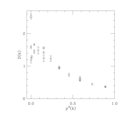
Figure 1: Plot of the three-momentum-space gluon propagator $D(k)$ (“fc”-data), as a function of the square of the lattice momentum $p^{2}(k)$. Data correspond to $V=16^{3}$ ($\Box$), $V=32^{3}$ ($\Diamond$) and $V=64^{3}$ ($\ast$), at $\beta=5.0$. Error bars are one standard deviation. Averages are taken over $40$ gauge-fixed configurations.

Our data [5, Table 2] show absence of Gribov noise for the gluon propagator. In fact, data corresponding to the minimal Landau gauge (absolute minima) are in complete agreement, within statistical errors, with those obtained in a generic Landau gauge (average “fc”). This happens even at $\beta=0$, where the number of Gribov copies is very large and Gribov noise, if present, is more easily detectable. On the contrary, a nonzero Gribov noise for the ghost propagator can be clearly observed [5, Table 3]. In particular, data corresponding to the absolute minima (average “am”) are constantly smaller than or equal to the corresponding “fc”-data. This effect is small but clearly detectable for the values of $\beta$ in the strong-coupling region. (This was not observed at $\beta=2.7$. However, at this value of $\beta$ almost no Gribov copies were produced, even for a lattice volume $V=16^{4}$, and therefore we cannot expect a difference between the two sets of data.) This result can been qualitatively explained [5]. As for the infrared behavior of these two propagators, the data for the ghost propagator show a pole “between” the zeroth-order perturbative behavior $p^{-2}$ — valid at large momenta — and the $p^{-4}$ singularity predicted in [4], but in agreement with the pole $p^{-2(1+s)}(0<s<1)$ recently obtained in ref. [6]. For the gluon propagator the data show, in the strong-coupling regime, a propagator decreasing as the momentum goes to zero. This anomalous behavior, predicted in [1, 4, 7], is still observable at $\beta=1.6$, if large volumes are considered [8]. This result is also observable in the scaling region in the three-dimensional case, and in the limit of large lattice volume (see Fig. 1). Finally, the behavior of the zero three-momentum-space gluon propagator is strongly affected by the zero-momentum modes of the gluon field [5, Fig. 2], as predicted in [9].

2 FOURIER ACCELERATION

In order to minimize the functional ${\cal E}_{U}[g]$ defined in eq. (2), and to reduce critical slowing-down, we can use the Fourier accelerated algorithm [10, 11]. With this algorithm the update is given by $g^{(new)}(x)\equiv R(x)\,g^{(old)}(x)$, where

$$R(x)\,\propto\,1\!\!\!\bot-{\widehat{F}}^{-1}\left[\,\frac{\alpha}{p^{2}(k)}\,{\widehat{F}}\left(\nabla\cdot A^{\left(g\right)}\right)\right](x)\;\mbox{.}$$ (3)

Here ${\widehat{F}}$ is a Fourier transform, $\alpha$ is a tuning parameter, $p^{2}(k)$ is the square of the lattice momentum, and $\nabla\cdot A$ is the lattice divergence of the gluon field $A_{\mu}$. However, this algorithm is of difficult implementation on parallel machines, due to the use of the fast Fourier transform (FFT).

Let us notice that ${\widehat{F}}^{-1}\,p^{-2}(k)\,{\widehat{F}}\,=\,\left(\,-\Delta\,\right)^{-1}$, where $\Delta$ is the lattice Laplacian operator. Thus, the FFT can be avoided by inverting $\Delta$ using an algorithm that requires the same computational work (i.e. $V\log N$), such as a multigrid (MG) algorithm with W cycle and piecewise-constant interpolation. At the same time, using MG, we can reduce the computational work with a good initial guess for the solution, and we can choose the accuracy of the solution. (With FFT the accuracy is fixed by the precision used in the numerical code.) We note that the tuning parameter $\alpha$ is usually fixed with an accuracy of a few percent, and thus the inversion of $\Delta$ should not require a very high accuracy either.

We started our simulations on an IBM RS-6000/340 workstation. We tested different types of multigrid cycles: $\gamma=0$ (Gauss-Seidel update), $\gamma=1$ (V cycle) and $\gamma=2$ (W cycle). We see that MG with $\gamma=2$, two relaxation sweeps on each grid, a minimum of two full multigrid sweeps for each version of $\Delta$, and an accuracy of $10^{-6}$, is equivalent to an FFT algorithm [12].

algorithm	$V$	GF-sweeps	CPU-time
FFT	$4^{4}$	$13.6\pm 0.3$	$36\pm 1$
MG	$4^{4}$	$13.7\pm 0.3$	$65\pm 3$
FFT	$8^{4}$	$16.1\pm 0.3$	$972\pm 16$
MG	$8^{4}$	$16.1\pm 0.3$	$1381\pm 49$
FFT	$16^{4}$	$20.0\pm 0.4$	$25254\pm 560$
MG	$16^{4}$	$19.9\pm 0.4$	$33797\pm 1114$

Table 1:            : Comparison between the FFT and MG algorithms at $\beta=\infty$.

In Table 1 we report results obtained at $\beta=\infty$ for the FFT algorithm, and for MG. Clearly, the two algorithms have a similar performance, showing a number of gauge-fixing sweeps increasing logarithmically with the lattice size $N$, and the CPU-time increasing as $N^{4}\log N$. We also did a test at $\beta=2.2$ (see Table 2). Again, MG is equivalent to the FFT algorithm.

algorithm	$V$	GF-sweeps	CPU-time
FFT	$8^{4}$	$333\pm 27$	$19998\pm 1236$
MG	$8^{4}$	$312\pm 25$	$18722\pm 1496$

Table 2:            : Comparison between the FFT and MG algorithms at $\beta=2.2$.

In order to parallelize, the idea is to use as the coarsest grid for the multigrid algorithm a grid with volume equal to or larger than the number of nodes of the parallel machine. For example, for an APE100 computer with $8^{3}$ nodes we implemented MG with the coarsest grid $8^{4}$. Then, on the coarsest grid, we can use a Gauss-Seidel relaxation if its volume is small. Otherwise we can use a Conjugate Gradient algorithm to relax the solution. (This combination MG+CG has been used in the past to accelerate MG on vector machines [13].) In this way, the computational work for the inversion of $\Delta$ still increases as V$\log$N, provided that we keep fixed the size of the coarsest grid. We tested this combination first on a workstation for a $16^{4}$ lattice with coarsest grid $8^{4}$ at $\beta=\infty$, performing two CG-sweeps when relaxing on the coarsest grid. We obtained $20.0\pm 0.4$ for the GF-sweeps, and $46281\pm 1732$ for the CPU-time. Therefore (see Table 1) the performance of this gauge-fixing algorithm is essentially equivalent to that of FFT and MG.

Similarly, the performance at $\beta=2.2$, for an $8^{4}$ lattice with coarsest grid $4^{4}$, is comparable to the performance of the FFT and MG algorithms (see Table 2): we obtained $314\pm 25$ for the GF-sweeps, and $23599\pm 1884$ for the CPU-time.

Finally, we implemented the MG+CG algorithm on an APE100 computer comparing its performance with a standard overrelaxation (OVE) and an unaccelerated local algorithm (the so-called Los Alamos algorithm, LOS) [11]. The number of gauge-fixing sweeps obtained, at $\beta=\infty$ and for lattice volume $16^{4}$, was $131\pm 3$ for LOS, $34.8\pm 0.5$ for OVE, and $16.4\pm 0.1$ for MG+CG. Clearly the MG+CG algorithm is able to reduce the number of gauge-fixing sweeps compared to the two local algorithms.

We plan to extend the tests on APE computers to larger lattice volumes.

References

- [1] V.N.Gribov, Nucl.Phys. B139 (1978) 1.
- [2] E.Marinari et al., Nucl.Phys. B362 (1991) 487; Ph. de Forcrand et al., Nucl.Phys. B (Proc.Suppl.) 20 (1991) 194.
- [3] G.Dell’Antonio and D.Zwanziger, Commun.Math.Phys. 138 (1991) 291; P. van Baal, hep-th/9511119, Proceedings of the QCD Workshop, Trento (Italy) 1995.
- [4] D.Zwanziger, Nucl.Phys. B412 (1994) 657.
- [5] A.Cucchieri, hep-lat/9705005, submitted to Nucl.Phys. B.
- [6] L. von Smekal et al., hep-ph/9707327.
- [7] D.Zwanziger, Nucl.Phys. B364 (1991) 127.
- [8] A.Cucchieri, hep-lat/9709015, submitted to Phys.Lett. B.
- [9] V.K.Mitrjushkin, Phys.Lett. B390 (1997) 293.
- [10] C.T.H.Davies et al., Phys.Rev. D37 (1988) 1581.
- [11] A.Cucchieri and T.Mendes, Nucl.Phys. B471 (1996) 263; A.Cucchieri and T.Mendes, Nucl.Phys. B (Proc.Suppl.) 53 (1997) 811; A.Cucchieri and T.Mendes, to be submitted to Nucl.Phys. B.
- [12] A.Cucchieri and T.Mendes, in preparation.
- [13] S.Solomon and P.G.Lauwers, Proceedings of the Workshop on Fermion Algorithms, Jul̈ich (Germany) 1991.