Real-time simulations and the electroweak phase transition

Abstract

We review recent developments in real-time simulations of SU(2)-Higgs theory near the electroweak transition and related topics.

1 Nonequilibrium phenomena

Nonequilibrium quantum field theory is important in various physical situations, such as domain formation during cosmological phase transitions and the properties of the electroweak transition in the early universe, or the QCD transition in heavy ion collisions. We concentrate in this talk on the SU(2)-Higgs model and the electroweak transition, which is relevant to theories of baryogenesis [1].

The description of nonequilibrium phenomena involves real time, as opposed to the imaginary time which is so useful for Monte Carlo computations in quantum field theory. Consider the time dependence of an observable $O$,

$$\langle O(t)\rangle=\mbox{Tr}\,\rho\,e^{iHt}\,O\,e^{-iHt}.$$

We know how to turn this operator expression into path integral form. It leads to phase factors $\exp(\pm iS)$, which are hopeless for Monte Carlo. Very hard is also the anaytical continuation of an imaginary time expression back to real time when the data for $\langle O(-i\tau)\rangle$ have errors, especially at ‘large’ times. A possible way out of these difficulties is the classical approximation.

2 Classical SU(2)-Higgs model on a spatial lattice

The action $S=\int dt\,(K-W)$, is given schematically by the kinetic energy

$$K = a\sum_{{\bf x}}\left[\frac{1}{z_{E}g^{2}}\,\mbox{Tr}\,(D_{0}U_{m})^{\dagger}D_{0}U_{m}\right.$$

$$\mbox{}\left.+\frac{1}{z_{\pi}}\,((\partial_{0}-iA_{0})\varphi)^{\dagger}(\partial_{0}-iA_{0})\varphi\right]_{{\bf x}}$$

and the potential energy

$$W = \frac{1}{a}\sum_{{\bf x}}\left[\sum_{mn}\frac{1}{g^{2}}\,\mbox{Tr}\,(1-U_{mn})\right.$$

$$\left.\mbox{}+(D_{m}\varphi)^{\dagger}D_{m}\varphi+\mu^{2}\varphi^{\dagger}\varphi+\lambda(\varphi^{\dagger}\varphi)^{2}\right]_{{\bf x}}.$$

Here time and $A_{0}$ are in physical units, but everything else is in lattice units $a=1$, with the exception of the explicitly indicated lattice spacing $a$.

Starting from an arbitrary initial field configuration the system will evolve in time over a region in phase space compatible with the conserved quantities. By ergodicity the field configurations sampled at large time intervals will be distributed according to the microcanonical ensemble. For large systems this is equivalent to the canonical ensemble: time average $\approx$ canonical average. Such averaging implies thermal equilibrium but we can still study small departures from equilibrium by looking at linear response functions $\langle O(t)O^{\prime}(0)\rangle$. Once the properties of these quantities are well understood we can turn to larger departures from equilibrium.

In the canonical description in the temporal gauge $A_{0}=0$, Gauss’ law $\delta S/\delta A_{0{\bf x}}^{\alpha}\equiv G_{{\bf x}}^{\alpha}=0$ has the status of a constraint. The hamiltonian takes the form $H=K+W$, with now

$$K=\frac{1}{a}\sum_{{\bf x}}\left[\frac{z_{E}}{2}\,g^{2}E^{\alpha}_{m}E^{\alpha}_{m}+z_{\pi}\pi^{\dagger}\pi\right]_{{\bf x}},$$

and the canonical partition function

$$Z=\int DED\pi DUD\varphi\,[\prod_{{\bf x}\alpha}\delta(G_{{\bf x}}^{\alpha})]\,\exp(-H/T).$$

By equipartition any initial configuration which is smooth on the lattice scale evolves into a ‘rough’ configuration, with temperature given by

$$\frac{\langle K\rangle}{V}=\frac{1}{2}\,(3\times 3+4-3)\,\frac{T}{a^{3}},$$

where $V$ is the volume and $\mbox{}-3$ reflects the three Gauss contraints per lattice site ${\bf x}$. The energy density diverges as the lattice spacing $a\to 0$ at fixed temperature, which is the notorious Rayleigh-Einstein-Jeans divergence [2].

3 Relation to dimensional reduction

The REJ divergence is not the only one, which can be seen by studying time-independent correlation functions like $\langle Q_{{\bf x}}(t)O_{{\bf y}}(t)\rangle$. It is then illuminating to integrate out the momenta by reintroducing $A_{0}$ into the canonical partition function, using $\int\exp(iA_{0{\bf x}}^{\alpha}G_{{\bf x}}^{\alpha})dA_{0{\bf x}}^{\alpha}$ to represent $\delta(G_{{\bf x}}^{\alpha})$. This leads via a rescaling of $A_{0}$ to the form of a three dimensional euclidean field theory,

$$Z_{\rm DR}=\int DA_{0}DUD\varphi\exp(-S_{\rm DR}),$$

with

$$S_{\rm DR} = \frac{W}{T}+\frac{1}{g^{2}aT}\sum_{{\bf x}}\left[\frac{1}{2}\,D_{m}A_{0}^{\alpha}D_{m}A_{0}^{\alpha}\right.$$ (2)

$$\left.\mbox{}+\frac{z_{E}/z_{\pi}}{4}\,g^{2}\varphi^{\dagger}\varphi A_{0}^{\alpha}A_{0}^{\alpha}\right]_{{\bf x}}.$$

Hence, for static quantities the classical theory is a dimensional reduction approximation to the quantum theory.

Dimensional reduction is an accurate approximation to a weakly coupled quantum theory in equillibrium at high temperature [3]. The reduced 3D theory is superrenormalizable which means that only mass counterterms are needed to obtain a finite theory. However, the above $S_{\rm DR}$ lacks a mass term for the ‘adjoint Higgs field’ $A_{0}$, since this is prohibited by the locality and gauge invariance of the classical action. In contrast, the usual derivation of the DR theory leads to additional terms of the form $\mu_{A}^{2}\mbox{Tr}\,A_{0}^{2}$ and $\lambda_{A}\mbox{Tr}\,A_{0}^{4}$. The coefficient $\lambda_{A}$ turns out to be negligible, but the fact that $\mu_{A}\equiv 0$ in the above $S_{\rm DR}$ means that the there is no possibility for an $A_{0}^{2}$ mass counterterm. It follows that the Debije screening mass $m_{D}$ associated with $A_{0}$ is divergent in perturbation theory, $m_{D}\propto 1/\sqrt{a}$. This need not be a disaster as $a\to 0$, because $A_{0}$ will simply decouple as it gets heavy. Indeed, $A_{0}$ is often integrated out explicitly as an additional approximation to dimensional reduction, because the renormalized Debije mass is large in perturbation theory.

The classical action evidently has to be interpreted as an effective action. Its parameters can be found by comparison with the dimensionally reduced quantum action with $A_{0}$ integrated out, which is known analytically through perturbative calculations. This means that $g^{2}$, $\lambda$ and $\mu^{2}$ are explicitly known in terms of the corresponding parameters of the quantum theory, and $a$ and $T$ [4]. In fact, $g^{2}\approx g^{2}_{\overline{MS}}(7T)$. This comparison also shows that the ratio $z_{E}/z_{\pi}\approx 1$ to a very good approximation.

We conclude, that for static observables the classical theory can approximate the quantum theory well. There is one undetermined parameter $z=z_{E}=z_{\pi}$. This parameter sets the time scale relative to the lattice spacing and it therefore plays a role in dynamical quantities, to which we turn next.

4 Dynamics

Time dependent quantities like $\langle O(t)O(0)\rangle$ can be computed in the microcanonical ensemble by solving the equations of motion on a computer. We can ‘help ergodicity’ by using the canonical ensemble for generating many initial configurations and averaging over these. Luckily, there are now two good solutions to the algorithmic problem of the implementation of the Gauss constraint [5, 6].

To see how well the classical theory may fare for dynamical quantities, one may turn to pertubation theory. The problem of solving perturbatively the equations of motion and averaging over initial conditions with the canonical ensemble has been studied in [7, 8] for $\phi^{4}$ scalar field theory. It was concluded in [8] that the mass counterterm needed to make static correlation functions finite is also sufficient for obtaining finite time-dependent correlation functions. The classical $\phi^{4}$ theory is renormalizable in this sense. Furthermore, after matching parameters of the classical theory to the dimensionally reduced quantum theory, the classical plasmon damping rate turned out to be identical to the quantum rate to leading order in the temperature and coupling [8] (see also [9]). Further analysis led to the conclusion that the classical $\lambda\phi^{4}$ theory can approximate the quantum theory for momenta and frequencies up to $O(\sqrt{\lambda}T)$, with corrections $O(\sqrt{\lambda})$ [10].

The procedure of solving equations of motion and averaging over initial conditions is awkward analytically. A more convenient formalism can be given which is a classical analogue of thermal field theory [10]. Alternatively one may use the imaginary time formalism of finite temperature quantum field theory and replace (after analytic continuation to real time) the Bose distribution by its high temperature approximation:

$$\frac{1}{2}\,+\frac{1}{e^{\omega/T}-1}\to\frac{T}{\omega}.$$ (3)

We assume this latter procedure for a brief discussion of the situation in gauge theories.

Figure 1: Gauge boson self energy diagrams.

Consider the gauge boson selfenergy
$\Pi_{\mu\nu}({\bf p},p^{0})=\Pi_{\mu\nu}^{(a)}({\bf p},p^{0})+\Pi_{\mu\nu}^{(b)}({\bf p},p^{0})$, as given by the diagrams in fig. 1, using the abelian Higgs model as a simple example. Both contributions (a) and (b) are linearly divergent (the quadratic divergence of the quantum theory is reduced to a linear divergence in the classical theory by (3)). Because of gauge invariance we may expect cancelations. Indeed, for external frequency $p^{0}=0$ the fields are static and therefore the spatial components $\Pi_{mn}^{(a)}({\bf p},0)$ and $\Pi_{mn}^{(b)}({\bf p},0)$ are related by a Ward identity of the dimensionally reduced theory. As a consequence, their sum $\Pi_{mn}({\bf p},0)$ is finite. However, for $p^{0}\neq 0$, the cancellation is incomplete and $\Pi_{mn}({\bf p},p^{0})$ turns out to be linearly divergent, in both real and imaginary parts. This may seem unfamiliar because in the quantum theory at zero temperature the Ward indentity reduces a quadratic divergence into a logarithmic divergence for all momenta. The reason such reduction does not follow here is that at finite temperature $\Pi_{mn}({\bf p},p^{0})$ is not analytic at ${\bf p}=0$ for $p^{0}\neq 0$. This is related to the physical process of Landau damping and a detailed physical picture has been developed by Arnold [11] which is also valid in the nonabelian case (on the lattice, measure-effects end up only into the momentum independent $\Pi_{\mu\nu}^{(b)}$).

The momentum dependence of the divergent terms is complicated, typically of the hard thermal loop form $\ln[(p^{0}+|{\bf p}|)/(p^{0}-|{\bf p}|)]$. This means that the divergencies in classical gauge theory are nonlocal in spacetime (in contrast to scalar field theory), which suggests nonlocal counterterms. This does not look attractive, although it may be possible to introduce new degrees of freedom to re-express such counterterms in local form. The situation is complicated, however, by the fact that on the lattice the divergencies lack rotational covariance [7, 11].

A different point of view prevails, in which the lattice spacing is supposed to stay finite, of order of the inverse temperature (the linear divergence $\propto g^{2}T/a$ is cured to $\propto g^{2}T^{2}$ in the quantum theory), and where the hard thermal loop physics is to be added ‘by hand’. There are difficulties with double counting, but practical proposals [12] are being pursued. Yet another approach consists of deriving an effective theory in which high frequency modes are subdominant, such that regulator effects vanish as the lattice spacing goes to zero [13].

In conclusion, for time-dependent quantities the classical model suffers from hard thermal loop effects which have lattice artefacts and which are divergent as the lattice spacing goes to zero. This is also relevant for Lyapunov exponents (cf. the brief remarks in [4]). Awaiting a solution of these problems, we still may expect to obtain useful information with the classical model at finite lattice spacing, provided the results are interpreted with care [11].

5 Sphaleron rate

The sphaleron rate, plays an important role in theories of baryogenesis [1]. It is the real time analogue of the topological susceptibility in imaginary time,

$$\Gamma=\frac{1}{t}\,\langle\left[\int_{0}^{t}dx^{0}\int d^{3}x\,\frac{\mbox{Tr}\,F\tilde{F}}{16\pi^{2}}\right]^{2}\rangle,\;\;\;t\to\infty,$$ (4)

in continuum notation. The usual expectations have been

$$\kappa \equiv \frac{\Gamma/V}{(\alpha_{W}T)^{4}},\;\;\;\alpha_{W}=\frac{g^{2}}{4\pi},$$ (5)

$$\propto \exp[-E_{s}(T)/T],\;\;\;T<T_{c},$$ (6)

$$\approx \mbox{const},\;\;\;\;\;\;\;\;\;\;\;\;\;\;\;\;\;\;\;T>T_{c},$$ (7)

where $E_{s}(T)$ is the temperature dependent sphaleron energy (of order 10 TeV for $T=0$, vanishing near $T_{c}$) and $\mbox{const}=O(1)$. The prefactors of the exponential sphaleron suppression (6) have been calculated analytically and the main problem for the numerical simulations is the computation of $\kappa$ above $T_{c}$. Recent work in pure SU(2) gauge theory [14] and in SU(2)-Higgs theory [4] using the same numerical implementation found $\kappa\approx 1.1$ in the high temperature phase. Furthermore, the results did not appear to depend on the lattice spacing. This is quite remarkable: a reduction of $a$ by a factor 0.6 caused $\Gamma/V$ to fall by factor $(0.6)^{4}\approx 0.13$, in both phases [4]. However, the expected sphaleron suppression was not observed in the low temperature phase, and indeed the results are considered to be wrong. The reason is that the imperfections of the ‘naive’ lattice implementation used for $\mbox{Tr}\,F\tilde{F}$ imply not only the need for a multiplicative renormalization, but also a subtractive renormalization for the rate; these were not taken into account. Such a subtraction has been controversial in euclidean lattice QCD, but in practise it appears to work well [15].

Recently, there have been two new computations using improved methods for obtaining $\Gamma$ [16, 17, 18], but before presenting these it is useful to mention new theoretical analysis questioning the lorical $\alpha_{W}$ independence of ‘const’ in (7). Arnold, Son and Yaffe (ASY) proposed the following picture [19]:

the nonperturbative processes important for $\Gamma$ occur on the typical momentum scale $g^{2}T$; however, due to Landau damping, the corresponding frequencies are not of the order $g^{2}T$, but $g^{4}T$.

Hence, the prediction is $\Gamma/V\approx\mbox{const}^{\prime}\,g^{2}\,(g^{2}T)^{4}$ or $\kappa\propto g^{2}$ as $g^{2}\to 0$, in contrast to the lore that $\kappa$ in (7) is practically independent of $g^{2}$.

Now $g^{2}T$ is the natural classical (dimensional reduction) scale for static processes ($H/T=\int d^{3}x\,\mbox{Tr}\,F_{mn}F_{mn}/4g^{2}T+\cdots$), but the extra factor of $g^{2}$ can only be supplied in a given regularization. On the lattice this involves the combination $\beta\equiv 4/g^{2}aT$ (recall (2)). So the prediction is that $\kappa\propto\beta^{-1}$, i.e. $\propto a$! Physically, the damping in the classical theory diverges as $a\to 0$, as discussed in the previous section, and then nothing moves anymore.

A detailed study of lattice effects in the classical theory by Arnold [11] suggests that not all is lost: we should readjust the time scale in the classical theory proportional to the ratio of damping rates of the quantum and classical theory. He obtained the following matching relation:

$$\kappa\approx 3.2\,\alpha_{W}\,\beta\,\kappa_{\rm class},$$ (8)

with an estimated error of about 30 % due to the cubic anisotropy of the lattice.

Figure 2: Data for $\beta\kappa_{\rm class}$ versus $\beta^{-1}$. The straight lines are fits to the MT data [16]: $\kappa_{\rm class}=25.1\,\beta^{-1}-56.7\,\beta^{-2}$ (upper) and $\kappa_{\rm class}=23.6\,\beta^{-1}-78.1\,\beta^{-2}$ (lower). The AK data are connected by lines to guide the eye; lower: ref. [17], upper: ref. [18].

The new methods for the computation of $\Gamma$ use cooling (Ambjørn and Krasnitz (AK) [17, 18]) or computing winding numbers of gauge transformations (Moore and Turok (MT) [16]). With either method the rate in the low temperature phase was found too small to be measureable, which is what one expects because of the sphaleron suppression (6). Fig. 2 summarizes the results for $\kappa_{\rm class}$ in the high temperature phase, in the form of $\beta\kappa_{\rm class}$ as a function of $\beta^{-1}$. The lower MT data are perturbatively corrected for some discretization errors. The AK data should be compared with the upper MT data, and they can be seen to be compatible, but the trend as a function of $\beta$ is different. If $\kappa_{\rm class}$ indeed vanishes proportional to $a$ we expect $\beta\kappa_{\rm class}$ to approach a constant as $\beta^{-1}\to 0$. This is clearly suggested by the MT data which can be fitted very well by a straight line (the slope represents $O(a^{2})$ corrections), but not by the AK data, for which $\kappa_{\rm class}$ itself and not $\beta\kappa_{\rm class}$ is approximately constant. Given the much larger leverage in the MT data one may tentatively conclude that $\kappa_{\rm class}\sim\beta^{-1}$. Of course, smaller $\beta^{-1}$ are desirable to confirm this behavior, or not. However, small volume AK results also show $\kappa_{\rm class}\propto\beta^{-1}$ [17]. Using (8) and the corrected MT data the tentative conclusion is then $\kappa\approx 76\,\alpha_{W}$.

Figure 3: The autocorrelator $C_{H}(t)$ in the Higgs phase for $T/T_{c}=0.85$, $aT=0.96$ (small amplitude) and $T/T_{c}=0.78$, $aT=0.41$ (large amplitude). The time is in lattice units.

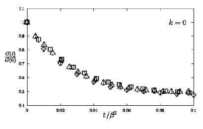
Figure 4: Zero momentum gauge field correlation function in Coulomb gauge, $C_{A}(t)/C_{A}(0)$ versus $t/\beta^{2}$, for $\beta=10$, 12, 14; ref. [17].

6 Autocorrelation functions

Apart from the correlation (4) used for the computation of the sphaleron rate there is very little nonperturbative information on time-dependent correlation functions. Correlators $C_{O}=\langle O(t)O(0)\rangle$ of gauge invariant fields

$$O\to\varphi^{\dagger}\varphi\equiv H,\;\;\;\to i\mbox{Tr}\,\phi^{\dagger}(\partial_{k}-iA_{k})\phi\tau_{\alpha}\equiv W^{\alpha}_{k},$$

($\phi$ is the matrix version of the doublet $\varphi$) have been computed at zero momentum [20]. Their interpretation may be guided by perturbation theory. In the Higgs phase $H$ and $W_{k}^{\alpha}$ are equivalent to $\varphi$ and $A_{k}^{\alpha}$, to lowest order, but in the plasma (high temperature) phase the interpretation is not so straightforward. In particular the analogy with the confinement phase of QCD, which holds for time-independent correlation functions and which suggests pole dominance by confined states, appears to be misleading in this time-dependent case. Furthermore, there is to my knowledge no analogue of the zero temperature ‘theorem of the arbitrariness of the interpolating field’.

Fig. 3 shows an example of $C_{H}$ in the Higgs phase. Similar results were obtained for $C_{W}(t)$. From the damped oscillations ‘plasmon’ frequencies and damping rates $\omega$ and $\gamma$ were extracted by fitting to a pole dominance form $C(t)=R\exp(-\gamma t)\cos(\omega t+\alpha)+\mbox{background}$. In the plasma phase the correlators are noisier; pole dominance is questionable and the extraction of $\gamma$ is difficult especially for $H$. The resulting $\omega$ and $\gamma$ appear to be approximately independent of the lattice spacing. Closer examination in the Higgs phase reveals, however, that the data for $\omega_{W}$ are compatible with a weak lattice spacing dependence expected from the perturbative $1/\sqrt{a}$ divergence. On the other hand, the damping rates are not divergent to leading order and both $\gamma_{H}$ and $\gamma_{W}$ turn out to have magnitudes similar to the analytic results in the quantum theory.

Ambjørn and Krasnitz [17] studied correlators of the gauge field itself in Coulomb gauge, $O\to A_{k}^{\alpha}$, for various momenta ${\bf p}$, in pure SU(2) gauge theory. These are better suited for comparison with perturbation theory and currently a hot issue is if the ASY analysis [11, 19] applies. This suggests overdamped correlation functions (which do not oscillate), while the classical divergence will show up in time scales increasing $\propto\beta$, i.e. in lattice units $\propto\beta^{2}$. The analysis applies to a regime $p_{0}^{2}\ll{\bf p}^{2}\ll T^{2}$, which is hard to satisfy in current simulations. Surprisingly the characteristics of overdamping and lattice time scale $\propto\beta^{2}$ shows up even for ${\bf p}=0$, cf. Fig. 4. This remains to be explained.

We have not shown here the richer structures found in the correlation functions in the plasma phase [20, 17], which are currently being analyzed [21, 22].

7 Dynamics of the phase transition

In a very stimulating paper [23], Moore and Turok studied the real time properties of the electroweak phase transition by numerical simulation. They obtained the drag coefficient for the moving wall between the Higgs and plasma phase, $\eta=\mbox{pressure}/\mbox{wall velocity}$, from the fluctuations of the wall position via a fluctation-dissipation argument. Another computation was the change in $\int F\tilde{F}$ under influence of a chemical potential related fermion production, in moving walls. There were several other interesting results and techniques, but there is no more space here for an illustration.

I thank Gert Aarts, Peter Arnold and Alex Krasnitz for useful discussions.

References

- [1] V.A. Rubakov, M.A. Shaposhnikov, hep-ph/9603208.
- [2] A. Pais, “Subtle is the Lord …”, sect. 19b. Oxford Unversity Press 1982.
- [3] K. Rummukainen, Nuc. Phys. (Proc. Suppl.) 53 (1997) 30.
- [4] W.H. Tang, J. Smit, Nucl. Phys. B482 (1996) 265.
- [5] A. Krasnitz, Nucl. Phys. B455 (1995) 320;
- [6] G.D. Moore, Nucl. Phys. B480 (1996) 657.
- [7] D. Bödeker, L. McLerran, A. Smilga, Phys. Rev. D52 (1995) 4675.
- [8] G. Aarts, J. Smit, Phys. Lett. B393 (1997) 395.
- [9] W. Buchmüller, A. Jakovác, hep-ph/9705452.
- [10] G. Aarts, J. Smit, hep-ph/9707342.
- [11] P. Arnold, Phys. Rev. D 55 (1997) 7781.
- [12] C.R. Hu, B. Müller, hep-ph/9611292.
- [13] D.T. Son, hep-ph/9707351.
- [14] J. Ambjørn, A. Krasnitz, Phys. Lett. B362 (1995) 97.
- [15] B. Allés, these proceedings.
- [16] G.D. Moore, N.G. Turok, hep-ph/9703266.
- [17] J. Ambjørn, A. Krasnitz, hep-ph/9705380.
- [18] A. Krasnitz, these proceedings.
- [19] P. Arnold, D. Son, L.G. Yaffe, Phys. Rev. D55 (1997) 6264.
- [20] W.H. Tang, J. Smit, hep-lat/9702017.
- [21] B. Bödeker, M. Laine, hep-ph/9707489.
- [22] P. Arnold, L.G. Yaffe, hep-ph/9709449.
- [23] G.D. Moore, N. Turok, Phys. Rev. D55 (1997) 6538.