Abstract. The metric of two-dimensional quantum gravity interacting with conformal matter is believed to collapse to a branched polymer metric when the central charge $c>1$. We show analytically that the spectral dimension, $d_{S}$, of such a branched polymer phase is ${4\over 3}$. This is in good agreement with numerical simulations for large $c$.

1 Introduction

The nature of the dimensionality of the manifolds appearing in euclidean quantum gravity ensembles has attracted considerable attention recently [1, 2, 3, 4, 5, 6, 7]. There are, in principle, many ways of defining the dimension; on smooth regular manifolds we expect every definition to yield the same value (for example 2 if the system is “two-dimensional”). However the euclidean quantum gravity ensembles contain many members which are very far from smooth, often showing some kind of fractal structure, and different definitions of dimension probe different global aspects of the geometry. Thus they can (and sometimes do) yield different numerical values.

Although these questions are of very general applicability by far the most complete studies of the notion of dimension have been conducted for two-dimensional euclidean quantum gravity (here “two-dimensional” means that every manifold in the ensemble is of dimension two in terms of the standard mathematical definition of a manifold). The ensemble is defined at fixed volume (which we denote the canonical ensemble, CE for short) by the partition function

$${}Z(V;\lambda)=\int Dg\,\delta\left(\int d^{2}\xi\,{\sqrt{g}}-V\right)\exp\left(-S_{eff}(g;\lambda)\right)$$ (1)

where the functional integral runs over all physically inequivalent metrics $g$ with the volume constrained by the delta-function to be $V$. The functional $S_{eff}(g;\lambda)$ is the effective action obtained for the metric after integrating out all matter fields and $\lambda$ represents any parameters (for example the central charge $c$) describing the matter field theory. Expectation values are given by

$${}{\left\langle\cdot\right\rangle}_{CE}=\frac{1}{Z(V;\lambda)}\int Dg\,(\cdot)\,\delta\left(\int d^{2}\xi\,{\sqrt{g}}-V\right)\exp\left(-S_{eff}(g;\lambda)\right)$$ (2)

with the understanding that it only makes sense to calculate the expectation values of reparametrization invariant quantities. We can also define a grand canonical ensemble (or GCE) partition function

$${}{\mathcal{Z}}(\mu;\lambda)=\int_{0}^{\infty}e^{-\mu V}Z(V;\lambda)\,dV.$$ (3)

In practice nearly all the available results about the dimensionality of the manifolds in these ensembles have been obtained in the discretized formulation [8, 9, 10]. The functional integral over metrics of a given volume is replaced by the sum over all triangulations (or, more generally, graphs), ${\mathcal{G}}$, with the number of vertices, $N_{{\mathcal{G}}}$, fixed so that the CE partition function is

$${}Z(N;\lambda)=\sum_{{{\mathcal{G}}}}\delta_{N,N_{{\mathcal{G}}}}\exp\left(-S_{eff}({{\mathcal{G}}};\lambda)\right)$$ (4)

and expectation values given by

$${}{\left\langle\cdot\right\rangle}_{CE}=\frac{1}{Z(N;\lambda)}\sum_{{{\mathcal{G}}}}\delta_{N,N_{{\mathcal{G}}}}(\cdot)\exp\left(-S_{eff}({{\mathcal{G}}};\lambda)\right).$$ (5)

To calculate the GCE partition function the integral over $V$ in (3) is replaced by a sum over $N$.

Two different notions of dimension have been considered in detail. The first is the “Hausdorff dimension”, $d_{h}$, which is defined by considering the volume of space, $d\tau$, contained in a shell of geodesic radius $R$ and thickness $dR$; provided that $R$ is much bigger than the short distance cut-off and much smaller than the characteristic linear geodesic size (which is $V^{1/\nu}$ for some exponent $\nu$) we expect that

$${}{\left\langle d\tau\right\rangle}_{CE}\sim R^{d_{h}-1}dR.$$ (6)

For $c=0$ an analytic calculation has been done and it is found that $d_{h}=4$ [2]. For other central charges $c>0$ the situation is still unclear but numerical results indicate that $d_{h}=4$ for unitary $c<1$ theories [5] and there is some analytic support for this [4]. For $c>1$ it is believed that the ensemble of universes collapses to a branched-polymer (BP) like phase; for a pure BP ensemble analytic calculation shows that $d_{h}=2$ [11] which is in very good agreement with numerical simulation for $c=5$ [7] (which seems to be the value of $c$ above which all these results change very little).

The second notion of dimension which has been investigated is the “spectral dimension”, $d_{S}$. This is defined for a given smooth metric $g$ on a d-dimensional manifold by the behaviour of the coincidence limit of the heat kernel $K_{g}(t;\xi,\xi^{\prime})$ for which it is known that

$${}K_{g}(t;\xi,\xi)=\frac{1}{t^{d/2}}\sum_{r=0}^{\infty}t^{r}a_{r}(\xi)$$ (7)

where the functions $a_{r}(\xi)$ are reparametrization invariant, see e.g. [12]. Thus in the quantum gravity ensemble we can define $d_{S}$ by

$${}{\left\langle K_{g}(t;\xi,\xi)\right\rangle}_{CE}\sim\frac{1}{t^{d_{S}/2}}$$ (8)

for $t$ small enough that the random walks generated by the Laplacian do not probe the finite size structure of the manifolds. In the discretized formulation we consider a random walk on a graph ${\mathcal{G}}$ with $N$ sites [7]; the random walker moves from one lattice point to one of its neighbours at each time step with equal probabilities corresponding to diffusion governed by the Laplacian of the graph. Letting the probability that the walker has returned to the starting point $i$ after $t$ steps be $P_{{\mathcal{G}}}(i;t)$ we can define $d_{S}$ by

$${}P_{N}(t)={\left\langle N^{-1}\sum_{i=1}^{N}P_{{\mathcal{G}}}(i;t)\right\rangle}_{CE}\sim\frac{1}{t^{d_{S}/2}}.$$ (9)

This behaviour is expected to hold provided $0\ll t\ll N^{1/\Delta}$ for some exponent $\Delta$ so that discretization and finite size effects are avoided. Numerical simulations show that $d_{S}\approx 2$ for $c=0$ and that as $c$ increases $d_{S}$ decreases [7]. It was conjectured in [7] that $d_{h}=2d_{S}$ for all values of $c$. This would imply that if the large $c$ phase is a BP phase then it has $d_{S}=1$. The purpose of this paper is to compute $d_{S}$ analytically for a pure branched polymer phase in order to check this conjecture and provide some definite result with which to compare the numerical simulations.

This paper is organized as follows. In section 2 we explain how $d_{S}$ which is defined in the CE can be calculated in the GCE. In section 3 we define the branched polymer ensemble and find relations satisfied by the return probabilities. In section 4 we do the GCE sum and show that $d_{S}={4\over 3}$. Section 5 contains the proofs of various results used in section 4; some technicalities are relegated to the appendix. Finally in section 6 we discuss our result and its connection to other spectral dimension problems (in particular on percolation clusters) that have been considered in the past.

2 Spectral dimension in the CE and the GCE

Our calculation of the spectral dimension for the BP ensemble (which we will define carefully in section 3) depends crucially upon the relationship between the CE and the GCE. This is most easily understood in the following way (we assume from now on that we are working with the discretized formulation). Consider first the CE; at very large times $t\gg N^{\Delta}$, where $\Delta$ is a suitable exponent, the walk will have uniform probability of being at any of the $N$ lattice sites (essentially this is just the contribution of the zero mode of the Laplacian) so

$${}\lim_{t\to\infty}P_{N}(t)=\frac{1}{N}.$$ (10)

At much smaller times we expect the behaviour (9) so that

$${}\lim_{N\to\infty}P_{N}(t)\sim\frac{1}{t^{d_{S}/2}}$$ (11)

A suitable interpolating function between these two limits is

$${}P_{N}(t)=\frac{1}{N}+\frac{a}{t^{d_{S}/2}}\exp\left(-\frac{t}{N^{\Delta}}\right)$$ (12)

where $a$ is a constant. From this we can compute the generating function

$${}{\bar{P}}_{N}(y)=\sum_{t=0}^{\infty}y^{t}P_{N}(t)\approx\frac{1}{N}\frac{1}{1-y}+\frac{a}{(1-y+N^{-\Delta})^{1-d_{S}/2}}$$ (13)

where we have assumed that $d_{S}<2$ and only written the dominating terms in ${\bar{P}}_{N}(y)$ as $y\uparrow 1$ and $N\to\infty$. Note the appearance of the simple pole at $y=1$ as a consequence of the zero mode and that the rest of ${\bar{P}}_{N}(y)$ is analytic at $y=1$ for finite $N$. Defining ${\bar{P}}\,^{\prime}_{N}(y)$ to be ${\bar{P}}_{N}(y)$ with the contribution of the zero mode subtracted (which we will find is straightforward in our actual calculation) we see that

$${}\lim_{N\to\infty}{\bar{P}}\,^{\prime}_{N}(y)=\frac{a}{(1-y)^{1-d_{S}/2}}$$ (14)

so that, as we might expect, the non-analyticity associated with $d_{S}$ appears only in the thermodynamic limit. Note that we also have that at large $N$

$${}{\bar{P}}\,^{\prime}_{N}(1)\sim N^{\Delta(1-d_{S}/2)}.$$ (15)

This result depends only on there being a cut-off in the $t^{-d_{S}/2}$ behaviour at $t\sim N^{\Delta}$ and not on its particular form.

In the GCE the natural quantity to compute is

$${}{\mathcal{P}}(z,y)=\sum_{{\mathcal{G}}}z^{N_{{\mathcal{G}}}}\sum_{t=0}^{\infty}y^{t}P_{{\mathcal{G}}}(i;t)$$ (16)

where the sum runs over all graphs ${\mathcal{G}}$ in the ensemble, $N_{{\mathcal{G}}}$ is the number of points in ${\mathcal{G}}$ and, as before, $P_{{\mathcal{G}}}(i;t)$ is the return probability of a walker on ${\mathcal{G}}$ returning to site $i$ after $t$ steps (in general one would also sum over starting points $i$ but in the case of branched polymers it is sufficient to consider walks starting at the root and summation over $i$ is not necessary). The function ${\mathcal{P}}$ is related to the CE quantity ${\bar{P}}_{N}(y)$ through

$${}{\mathcal{P}}(z,y)=\sum_{N}z^{N}Z(N;\lambda){\bar{P}}_{N}(y).$$ (17)

We expect that for large $N$ the CE partition function behaves as

$${}Z(N;\lambda)\sim N^{\gamma_{str}-2}z_{0}^{-N}$$ (18)

where $z_{0}$ is a constant and $\gamma_{str}\leq{1\over 2}$. It follows that the coefficient of the pole term is finite at criticality (ie at $z\uparrow z_{0}$ where graphs of arbitrary size contribute). Dropping the pole term to get

$${}{\mathcal{P}}^{\prime}(z,y)=\sum_{N}z^{N}Z(N;\lambda){\bar{P}}\,^{\prime}_{N}(y)$$ (19)

and approximating the sum over $N$ by an integral we find, using (13),

$${}{\mathcal{P}}^{\prime}(z,y)\sim\left(1-\frac{z}{z_{0}}\right)^{\beta}\Phi\left(\frac{1-y}{\left(1-\frac{z}{z_{0}}\right)^{\Delta}}\right)$$ (20)

where the prefactor exponent $\beta$ is given by

$${}\beta=1-\gamma_{str}+\Delta\left(\frac{d_{S}}{2}-1\right)$$ (21)

and the function $\Phi$ by

$${}\Phi(v)=\int_{1}^{\infty}\frac{ae^{-x}}{(v+x^{\Delta})^{1-d_{S}/2}}\,dx.$$ (22)

Note that $\Phi(v)$ is analytic for $v\geq 0$ with $\Phi(0)=O(1)$. The result (20) describes correctly the singularity of ${\mathcal{P}}^{\prime}(z,y)$ at $z=z_{0}$ provided that the prefactor diverges as $z\uparrow z_{0}$; if it does not then we consider instead a higher derivative of ${\mathcal{P}}^{\prime}(z,y)$ with respect to $z$. We draw three lessons from (20):

1. It is not the case that

   $${}{\mathcal{P}}^{\prime}(z,y)\stackrel{{\scriptstyle y\to 1}}{{\sim}}\frac{1}{(1-y)^{1-d_{S}/2}}$$ (23)

   In fact, for $z<z_{0}$, ${\mathcal{P}}^{\prime}(z,y)$ is an analytic function on a neighbourhood of $y=1$.

2. The exponent $\Delta$ is a gap exponent; that is the $n+1$st derivative of ${\mathcal{P}}^{\prime}(z,y)$ with respect to $y$ is more divergent than the $n$th derivative as $z\uparrow z_{0}$ by a factor $(1-z/z_{0})^{-\Delta}$.

3. If we can compute the prefactor exponent, $\beta$, and the gap exponent $\Delta$ in the GCE we can find $d_{S}$ using (21).

This discussion is based on the interpolating ansatz (12) and the reader might worry that it is not completely general. In fact, although the ansatz is useful for pedagogical purposes, we shall show in section 4.2 that it is not necessary.

3 Branched Polymers

3.1 The Polymer Ensemble

In this work we will restrict our attention to polymers which have vertices of order one or of order three and in which one vertex of order one, called the root, is distinguished. This is the simplest case of the generic rooted branched polymer ensemble [11]. The simplest polymer, ${\mathrm{B}}_{0}$, consists of one link joining the root, labelled “0”, to one other vertex of order one which we label “1” as shown in fig.1.

Figure 1: The elementary polymer ${{\mathrm{B}}}_{0}$.

The ensemble of all polymers, ${\mathcal{B}}$, is generated by the statements:

1. The only element of ${\mathcal{B}}$ consisting of one link is ${\mathrm{B}}_{0}$.

2. Any two polymers, ${\mathrm{B}}_{1}$ and ${\mathrm{B}}_{2}$ may be combined to generate a new, and larger, polymer ${\mathrm{B}}_{3}={\mathrm{B}}_{1}\cup{\mathrm{B}}_{2}$ as shown in fig.2.

Figure 2: The combination of polymers ${{\mathrm{B}}}_{1}$ and ${{\mathrm{B}}}_{2}$ to form ${{\mathrm{B}}}_{3}$.

It is clear that any polymer ${\mathrm{B}}\in{\mathcal{B}}$, ${{{\mathrm{B}}}}\neq{{{\mathrm{B}}}}_{0}$, has a unique decomposition into two constituent polymers ${\mathrm{B}}^{\prime}$ and ${\mathrm{B}}^{\prime\prime}$ by cutting just to the right of vertex “1” as shown in fig.3.

Figure 3: The unique decomposition of polymer ${{\mathrm{B}}}$ to its constituents ${{\mathrm{B}}}^{\prime}$ and ${{\mathrm{B}}}^{\prime\prime}$.

One characteristic of an element ${\mathrm{B}}$ of ${\mathcal{B}}$ is the number of order one vertices (not counting the root) which we will call the size and denote $N_{B}$; clearly we have

$${}N_{{\mathrm{B}}_{1}\cup{\mathrm{B}}_{2}}=N_{{\mathrm{B}}_{1}}+N_{{\mathrm{B}}_{2}}.$$ (24)

Letting $\Omega_{N}$ be the number of elements of ${\mathcal{B}}$ with a given size, $N$, we find

$${}\Omega_{N}=\sum_{M=1}^{N-1}\Omega_{M}\Omega_{N-M}$$ (25)

with $\Omega_{1}=1$. This is the recurrence relation for the Catalan numbers, $T_{N}$, so

$${}\Omega_{N}=T_{N}=\frac{(2N-2)!}{N!(N-1)!}.$$ (26)

For large $N$, the numbers $T_{N}$ have the asymptotic behaviour

$${}T_{N}\sim\frac{4^{N}}{N^{\frac{3}{2}}}.$$ (27)

Note that the number of vertices of order three is $N-1$, and hence the total number of vertices excluding the root is $2N-1$, so $N$ is a sensible measure of the volume of the system. We therefore expect on general grounds that $\Omega_{N}\sim N^{\gamma_{str}-2}\exp\mu_{0}N$; comparing with (27) we recover the well known result for branched polymers that $\gamma_{str}={1\over 2}$. The generating function of the Catalan numbers will appear repeatedly in the rest of this paper and is given by

$${}{\mathcal{T}}(z)=\sum_{N=1}^{\infty}z^{N}T_{N}={1\over 2}(1-\sqrt{1-4z}).$$ (28)

Note that this definition of ${\mathcal{B}}$ naturally connects ensemble members of different sizes suggesting that the Grand Canonical Ensemble (GCE), which contains polymers of all sizes, may be easier to calculate with than the Canonical Ensemble (CE) which contains polymers of fixed size; indeed (28) is nothing but the GCE partition function for ${\mathcal{B}}$ with the action $N_{{{\mathrm{B}}}}$.

3.2 Random Walks on Polymers

Since ${\mathcal{B}}$ is defined with a vertex of special status, the root, it is convenient to consider walks starting and ending at the root rather than summing over all vertices. This does not affect the value of $d_{S}$ because in fact half of all vertices have coordination number one like the root and are therefore equivalent as starting points. First consider an arbitrary polymer ${{{\mathrm{B}}}}\neq{{{\mathrm{B}}}}_{0}$. At $t=0$ a walker sets out from the root; at $t=1$, after taking one step, he/she is necessarily at the first vertex; for the next step one of the three links attached to the first vertex is chosen with uniform probability and the walk proceeds down that link. The process continues in this way with the step taken chosen with uniform probability from the possible steps. Now let $P_{{\mathrm{B}}}^{1}(t)$ be the probability that the walker returns to the root for the first time after $t$ steps, and let $P_{{{\mathrm{B}}}}(t)$ be the probability that, after $t$ steps, the walker is at the root. Note that both $P_{{\mathrm{B}}}^{1}(t)$ and $P_{{\mathrm{B}}}(t)$ are zero for odd $t$ and that $P_{{\mathrm{B}}}^{1}(0)=0$ because at least two steps are needed to return to the root for the first time. Clearly walks contributing to $P_{{\mathrm{B}}}(t)$ may be back at the origin for the first, second, third …. occasion so we have

$${}P_{{\mathrm{B}}}(t)=\delta_{t,0}+P_{{\mathrm{B}}}^{1}(t)+\sum_{t_{1}+t_{2}=t}P_{{\mathrm{B}}}^{1}(t_{1})P_{{\mathrm{B}}}^{1}(t_{2})+\ldots+\sum_{t_{1}+t_{2}+\ldots+t_{n}=t}\prod_{i=1}^{n}P_{{\mathrm{B}}}^{1}(t_{i})+\ldots\,.$$ (29)

Introduce the generating functions

$${\bar{P}}_{{\mathrm{B}}}(y)=\sum_{t=0}^{\infty}y^{t/2}P_{{\mathrm{B}}}(t)$$ (30)

and

$${\bar{P}}_{{\mathrm{B}}}^{1}(y)=\sum_{t=0}^{\infty}y^{t/2}P_{{\mathrm{B}}}^{1}(t).$$ (31)

We substitute (29) into (30) and then use (31) to obtain

$${\bar{P}}_{{\mathrm{B}}}(y) = 1+{\bar{P}}_{{\mathrm{B}}}^{1}(y)+({\bar{P}}_{{\mathrm{B}}}^{1}(y))^{2}+\ldots$$ (32)

$$= \frac{1}{1-{\bar{P}}_{{\mathrm{B}}}^{1}(y)}.$$

Let us now consider a polymer ${{\mathrm{A}}}\neq{{\mathrm{B}}}_{0}$ which is made by joining two polymers B and C, cf. fig.2. We want to relate the first return probability on A to the first return probabilities on its constituents B and C. A typical walk leaves the root and then goes out and back many times from the first vertex along B and C before finally returning to the root; an example is shown in fig.4.

Figure 4: Example of a walk contributing to the first return probability on polymer ${{\mathrm{A}}}={{\mathrm{B}}}\cup{{\mathrm{C}}}$.

Taking all these walks into account we find that

$$P_{{\mathrm{A}}}^{1}(t) = {1\over 3}\delta_{t,2}+\left({1\over 3}\right)^{2}\left(P_{{\mathrm{B}}}^{1}(t-2)+P_{{\mathrm{C}}}^{1}(t-2)\right)$$ (33)

$$+\left({1\over 3}\right)^{3}\sum_{t_{1}+t_{2}=t-2}\left(P_{{\mathrm{B}}}^{1}(t_{1})+P_{{\mathrm{C}}}^{1}(t_{1})\right)\left(P_{{\mathrm{B}}}^{1}(t_{2})+P_{{\mathrm{C}}}^{1}(t_{2})\right)+\ldots$$

$$\ldots+\left({1\over 3}\right)^{n+1}\sum_{t_{1}+\ldots+t_{n}=t-2}\prod_{i=1}^{n}\left(P_{{\mathrm{B}}}^{1}(t_{i})+P_{{\mathrm{C}}}^{1}(t_{i})\right)+\ldots\,.$$

Inserting (33) into (31) we get

$${\bar{P}}_{{\mathrm{A}}}^{1}(y) = {1\over 3}y+\left({1\over 3}\right)^{2}\left({\bar{P}}_{{\mathrm{B}}}^{1}(y)+{\bar{P}}_{{\mathrm{C}}}^{1}(y)\right)+\left({1\over 3}\right)^{3}\left({\bar{P}}_{{\mathrm{B}}}^{1}(y)+{\bar{P}}_{{\mathrm{C}}}^{1}(y)\right)^{2}+\ldots$$ (34)

$$\ldots+\left({1\over 3}\right)^{n+1}\left({\bar{P}}_{{\mathrm{B}}}^{1}(y)+{\bar{P}}_{{\mathrm{C}}}^{1}(y)\right)^{n}+\ldots$$

$$= \frac{y}{3-({\bar{P}}_{{\mathrm{B}}}^{1}(y)+{\bar{P}}_{{\mathrm{C}}}^{1}(y))}.$$

It is convenient to introduce a new quantity $h_{{\mathrm{A}}}(y)$ defined by

$${}h_{{\mathrm{A}}}(y)=\frac{1}{1-y}\left(1-{\bar{P}}^{1}_{{\mathrm{A}}}(y)\right).$$ (35)

We find from (32) that the return probability generating function on A is then given by

$${}{\bar{P}}_{{\mathrm{A}}}(y)=\frac{1}{1-y}\,\frac{1}{h_{{\mathrm{A}}}(y)}$$ (36)

and the recurrence relation for the first return probabilities (34) becomes

$${}h_{{\mathrm{A}}}(y)=\frac{1+h_{{\mathrm{B}}}(y)+h_{{\mathrm{C}}}(y)}{1+(1-y)\left(h_{{\mathrm{B}}}(y)+h_{{\mathrm{C}}}(y)\right)}.$$ (37)

Note that for the elementary polymer, ${\mathrm{B}}_{0}$, we have

$${}h_{{\mathrm{B}}_{0}}=1.$$ (38)

We can, at least in principle, generate ${\bar{P}}_{{\mathrm{B}}}(y)$ for every ${\mathrm{B}}\in{\mathcal{B}}$ from the recurrence (37) and the initial condition (38).

4 Random Walks in the GCE

4.1 The generating function

We define the GCE generating function

$${}{\mathcal{Q}}(z,y)=\sum_{{\mathrm{B}}\in{\mathcal{B}}}z^{N_{{\mathrm{B}}}}{\bar{P}}_{{\mathrm{B}}}(y)$$ (39)

which, because of (36), becomes

$${}{\mathcal{Q}}(z,y)=\frac{1}{1-y}\sum_{{\mathrm{B}}\in{\mathcal{B}}}z^{N_{{\mathrm{B}}}}\left(h_{{\mathrm{B}}}(y)\right)^{-1}.$$ (40)

First we will show that ${\mathcal{Q}}(z,y)$ has a simple pole at $y=1$ with finite residue provided $z\leq{1\over 4}$. From (37) we see easily by induction that the functions $h_{{{\mathrm{B}}}}$ are non-decreasing. It therefore suffices to show that the sum in (40) with $h_{{\mathrm{B}}}(y)$ replaced by $h_{{\mathrm{B}}}(1)$ converges. From (37) we have

$${}h_{{\mathrm{B}}\cup{\mathrm{C}}}(1)=1+h_{{\mathrm{B}}}(1)+h_{{\mathrm{C}}}(1).$$ (41)

From this, the initial condition (38), and the relation between the sizes (24), it follows that

$${}h_{{\mathrm{A}}}(1)=2N_{{\mathrm{A}}}-1.$$ (42)

Note that this quantity takes the same value for all polymers of a given size. Using (42) we have

$${}(1-y){\mathcal{Q}}(z,y)|_{y=1}=\sum_{N=1}^{\infty}\frac{z^{N}\Omega_{N}}{2N-1}$$ (43)

which converges for $z\leq{1\over 4}$ on account of (27).

As we discussed in section 2, the simple pole in ${\mathcal{Q}}(z,y)$ at $y=1$ arises from walks that are much longer than the size of the polymer; we expect to find these walks at an arbitrary point in the polymer with essentially uniform probability which in this case, according to (42), is $(2N_{{\mathrm{A}}}-1)^{-1}$. The information about $d_{S}$ is contained in the remaining (ie non-pole) part of ${\mathcal{Q}}(z,y)$ so we define a new function

$${\widetilde{{\mathcal{Q}}}}(z,y) = -\frac{d~{}}{dy}\left((1-y){\mathcal{Q}}(z,y)\right)$$ (44)

$$= \sum_{{\mathrm{B}}\in{\mathcal{B}}}z^{N_{{\mathrm{B}}}}\left(h_{{\mathrm{B}}}(y)\right)^{-2}\frac{dh_{{\mathrm{B}}}(y)}{dy}.$$

Now define

$${\widetilde{{\mathcal{Q}}}}_{n}(z) = {\left(\frac{d~{}}{dy}\right)}^{n}{\widetilde{{\mathcal{Q}}}}(z,y){\Bigg{|}_{y=1}}$$ (45)

$$= -\sum_{{{\mathrm{B}}}\in{\mathcal{B}}}z^{N_{{\mathrm{B}}}}{\left(\frac{d~{}}{dy}\right)}^{n+1}\frac{1}{h_{{\mathrm{B}}}(y)}{\Bigg{|}_{y=1}}.$$

Assuming for the moment that all these objects actually exist, then formally

$${}{\widetilde{{\mathcal{Q}}}}(z,y)=\sum_{n=0}^{\infty}\frac{(y-1)^{n}}{n!}{\widetilde{{\mathcal{Q}}}}_{n}(z).$$ (46)

We show in the appendix that this series is asymptotic but that it is not Borel summable. Nonetheless, we will argue in section 5 that the leading terms can be re-summed to an integral representation which is analytic in the region of interest. The absence of Borel summability means that such a function is not unique. However it can only differ from the true result by terms which have essential singularities at $y=1$ (and vanish there) and we do not expect these to affect the spectral dimension; so long as there is any power law scaling as $y\to 1$ any vanishing essential singularities are irrelevant.

Now let

$${}h_{{{\mathrm{B}}}}^{(n)}={\left(\frac{d~{}}{dy}\right)}^{n}h_{{\mathrm{B}}}(y){\Bigg{|}_{y=1}}.$$ (47)

Then

$${}-{\left(\frac{d~{}}{dy}\right)}^{n+1}\frac{1}{h_{{\mathrm{B}}}(y)}{\Bigg{|}_{y=1}}=\sum_{r=1}^{n+1}\frac{(-1)^{r+1}r!}{(h_{{{\mathrm{B}}}}^{(0)})^{r+1}}\sum_{{\mathcal{F}}(n+1,r)}(n+1;a_{1},\ldots a_{n+1})^{\prime}\prod_{i=1}^{n+1}(h_{{{\mathrm{B}}}}^{(i)})^{a_{i}}$$ (48)

where $(m;a_{1}\ldots a_{m})^{\prime}$ is the multinomial coefficient [13]

$${}(m;a_{1}\ldots a_{m})^{\prime}=\frac{m!}{(1!)^{a_{1}}\ldots(m!)^{a_{m}}a_{1}!\ldots a_{m}!}$$ (49)

and the summation region ${\mathcal{F}}(n+1,r)$ consists of all non-negative integers $a_{1},\ldots,a_{n+1}$ such that

$${}\sum_{k=1}^{n+1}ka_{k}=n+1,\quad\sum_{k=1}^{n+1}a_{k}=r.$$ (50)

Inserting (48) into (45) and reordering the sums gives

$${\widetilde{{\mathcal{Q}}}}_{n}(z) = \sum_{r=1}^{n+1}{(-1)^{r+1}r!}\sum_{{\mathcal{F}}(n+1,r)}(n+1;a_{1},\ldots a_{n+1})^{\prime}\left(\sum_{{{\mathrm{B}}}\in{\mathcal{B}}}z^{N_{{\mathrm{B}}}}\frac{\prod_{i=1}^{n+1}(h_{{{\mathrm{B}}}}^{(i)})^{a_{i}}}{(h_{{{\mathrm{B}}}}^{(0)})^{r+1}}\right).$$ (51)

Let us define

$${}H^{(n_{1},n_{2},\ldots,n_{p})}(z)=\sum_{{{\mathrm{B}}}\in{\mathcal{B}}}z^{N_{B}}\prod_{i=1}^{p}h_{{{\mathrm{B}}}}^{(n_{i})},\qquad p,n_{i}>0.$$ (52)

We will prove in section 5 that

$${}H^{(n_{1},n_{2},\ldots,n_{p})}(z)\simeq A^{(n_{1},n_{2},\ldots,n_{p})}(1-4z)^{{1\over 2}-p-{3\over 2}\sum_{i=1}^{p}n_{i}}$$ (53)

where the symbol $\simeq$ means the most singular part as $z\uparrow{1\over 4}$ and where $A^{(n_{1},n_{2},\ldots,n_{p})}$ is a constant. Using (42) we note that

$$H^{(a_{1}\otimes 1,a_{2}\otimes 2,\ldots,a_{n+1}\otimes n+1)}(z) = \left(2z\frac{\partial~{}}{\partial z}-1\right)^{r+1}\left(\sum_{{{\mathrm{B}}}\in{\mathcal{B}}}z^{N_{{\mathrm{B}}}}\frac{\prod_{i=1}^{n+1}(h_{{{\mathrm{B}}}}^{(i)})^{a_{i}}}{(h_{{{\mathrm{B}}}}^{(0)})^{r+1}}\right)$$ (54)

where by $q\otimes m$ we mean that the number $m$ appears $q$ times in the list. Using (53) and integrating $r+1$ times we find the leading singular behaviour of ${\widetilde{{\mathcal{Q}}}}_{n}(z)$ for $n\neq 0$ to be

$${\widetilde{{\mathcal{Q}}}}_{n}(z) \simeq (1-4z)^{-{3\over 2}n}\sum_{r=1}^{n+1}\frac{(-1)^{r+1}r!}{2^{r+1}}\frac{\Gamma({3\over 2}n)}{\Gamma({3\over 2}n+r+1)}$$ (55)

$$\times\sum_{{\mathcal{F}}(n+1,r)}(n+1;a_{1},\ldots a_{n+1})A^{(a_{1}\otimes 1,a_{2}\otimes 2,\ldots,a_{n+1}\otimes n+1)}.$$

When $n=0$ we obtain

$${\widetilde{{\mathcal{Q}}}}_{0}(z) = -{1\over 8}\log(1-4z).$$ (56)

Substituting (55) and (56) in (46) we see that the most singular part of ${\widetilde{{\mathcal{Q}}}}(z,y)$ as $z\uparrow{1\over 4}$ is the sum of a logarithmic piece and a function of $(1-y)(1-4z)^{-{3\over 2}}$. For the rest of the analysis it is more convenient to work with $\frac{\partial{\widetilde{{\mathcal{Q}}}}}{\partial z}$ which takes the form

$${}\frac{\partial{\widetilde{{\mathcal{Q}}}}}{\partial z}=\frac{1}{1-4z}{\widetilde{\Phi}}\left(\frac{1-y}{(1-4z)^{3\over 2}}\right)$$ (57)

for some function ${\widetilde{\Phi}}$. From now on in this paper we will be working with this most singular (as $z\uparrow{1\over 4}$) part of ${\widetilde{{\mathcal{Q}}}}$ unless otherwise stated. Note that from (57) we deduce that the gap exponent $\Delta={3\over 2}$.

4.2 Extracting $d_{S}$ from the GCE

The behaviour of ${\widetilde{{\mathcal{Q}}}}(z,1)={\widetilde{{\mathcal{Q}}}}_{0}(z)$ given by (56) can be used to place an upper bound on $d_{S}$ which we will need later. From (27), (39), (44) we have

$${}{\widetilde{{\mathcal{Q}}}}(z,1)=\sum_{N}N^{-{3\over 2}}(4z)^{N}{\bar{P}}^{\prime}_{N}(1).$$ (58)

Together with (56) this implies that ${\bar{P}}^{\prime}_{N}(1)\sim N^{1\over 2}$ at large $N$. But from (15) this can only happen if $d_{S}<2$.

As we discussed in section 2, the GCE generating function is related to the CE generating function by

$$\frac{\partial{\widetilde{{\mathcal{Q}}}}}{\partial z} = \frac{1}{u}{\widetilde{\Phi}}\left(\frac{1-y}{u^{\Delta}}\right)$$ (59)

$$= \int_{0}^{\infty}dx\,x^{\gamma_{str}-1}\,\Phi(1-y,x)\exp(-xu)$$

where, for convenience, we have introduced $u=1-4z$ and a continuous variable $x$ equivalent at integer values to $N$, the size of the system. Since we are looking for the asymptotic behaviour at large $N$ we can approximate the discrete sum over $N$ by a Laplace Transform in $x$; the difference will be sub-leading. The extra factor of $x$ appears in (59) compared to (18) because we are looking at $\frac{\partial{\widetilde{{\mathcal{Q}}}}}{\partial z}$ rather than ${\widetilde{{\mathcal{Q}}}}$; this makes life easier because it removes the possibility of a trivial divergence at small $x$. From (59) it follows that

$${}\Phi(1-y,x)=x^{1-\gamma_{str}}\phi((1-y)x^{\Delta})$$ (60)

for a suitable function $\phi$. To show this introduce new variables $u^{\prime}=u(1-y)^{-1/\Delta}$ and $x^{\prime}=x(1-y)^{1/\Delta}$ into (59) to get

$$\frac{1}{u^{\prime}}{\widetilde{\Phi}}\left(\frac{1}{u^{\prime\Delta}}\right)=(1-y)^{-(\gamma_{str}-1)/\Delta}\int_{0}^{\infty}dx^{\prime}\,x^{\prime\gamma_{str}-1}\Phi(1-y,\frac{x^{\prime}}{(1-y)^{1/\Delta}})\exp(-x^{\prime}u^{\prime})$$ (61)

but by setting $y=0$ and $u=u^{\prime}$ in (59) we also have

$${}\frac{1}{u^{\prime}}{\widetilde{\Phi}}\left(\frac{1}{u^{\prime\Delta}}\right)=\int_{0}^{\infty}dx\,x^{\gamma_{str}-1}\,\Phi(1,x)\exp(-xu^{\prime}).$$ (62)

Similar identities are valid for the derivatives of ${\widetilde{\Phi}}$ w.r.t. $z$ so

$${}\Phi(1,x)=(1-y)^{-(\gamma_{str}-1)/\Delta}\Phi(1-y,\frac{x}{(1-y)^{1/\Delta}})$$ (63)

and the result (60) follows. Now it is easy to see that $\Phi(1-y,x)$ must be a bounded quantity in $x>0$ for fixed $y<1$; we have

$$\Phi(1-y,N)=\frac{1}{T_{N}}\sum_{i=1}^{T_{N}}\sum_{t=0}^{\infty}y^{t}\left(P_{i}(t)-\frac{1}{2N-1}\right)$$ (64)

where the subtraction is to remove the pole term. Now $P_{i}(t)<1$ and $P_{i}(0)=1$ so we get

$$1-\frac{1}{2N-1}<\Phi(1-y,N)<\frac{1}{1-y}\left(1-\frac{1}{2N-1}\right).$$ (65)

It follows from (65) that $\lim_{x\to\infty}\Phi(1-y,x)$ must be finite for $y<1$ and this is compatible with (60) only if $\phi(s)$ behaves like,

$${}\phi(s)\stackrel{{\scriptstyle s\to\infty}}{{\sim}}s^{-(1-\gamma_{str})/\Delta}$$ (66)

and so we conclude that

$${}\lim_{x\to\infty}\Phi(1-y,x)\sim(1-y)^{-(1-\gamma_{str})/\Delta}.$$ (67)

Substituting in the values of $\gamma_{str}={1\over 2}$ and $\Delta={3\over 2}$ for the branched polymer ensemble ${\mathcal{B}}$ we obtain

$${}\lim_{x\to\infty}\Phi(1-y,x)\sim(1-y)^{-{1\over 3}}.$$ (68)

This is the generating function $\lim_{N\to\infty}{\bar{P}}^{\prime}_{N}(y)$ so we find that $\lim_{N\to\infty}P_{N}(t)\sim t^{-{2\over 3}}$ and hence that $d_{S}={4\over 3}$ (see (13) and (14)).

4.3 Sub-leading terms

There are two sources of subleading behaviour. The first is the corrections to the asymptotic form (66) which must be like

$${}\phi(s)\stackrel{{\scriptstyle s\to\infty}}{{\sim}}s^{-(1-\gamma_{str})/\Delta}\left(1+\frac{const}{s^{\epsilon}}\right),\quad\epsilon>0$$ (69)

in order for (65) to be satisfied. The correction term is more singular as $y\uparrow 1$, and so has smaller $d_{S}$, but is suppressed by $N^{\epsilon}$ in the thermodynamic limit. This is expected because we know that there are members of ${\mathcal{B}}$ (for example the linear polymers which are basically infinite chains with finite sized outgrowths) which have $d_{S}=1$ but are thermodynamically insignificant.

The second source of subleading behaviour is the corrections to (53) which, as we will show in section 5, take the form $u^{\delta+{1\over 2}-p-{3\over 2}\sum_{i=1}^{p}n_{i}}$ with $\delta={1\over 2},1,{3\over 2}\ldots$. The consequence of this is that (57) is modifed to

$${}\frac{\partial{\widetilde{{\mathcal{Q}}}}}{\partial z}=\frac{1}{1-4z}{\widetilde{\Phi}}\left(\frac{1-y}{(1-4z)^{3\over 2}}\right)+\sum_{i}\frac{1}{(1-4z)^{1-\delta_{i}}}{\widetilde{\Phi}}_{i}\left(\frac{1-y}{(1-4z)^{3\over 2}}\right)$$ (70)

where the functions $\Phi_{i}(1-y,N)$ have the same upper bound as $\Phi(1-y,N)$, see (65). Repeating the manipulations of section 4.2, and assuming that the $i$’th term in (70) makes a contribution which survives as $N\to\infty$ we find by the arguments of the previous sub-section that it has a spectral dimension

$${}d_{S}^{i}=2+{2\over 3}(2\delta-1)\geq 2.$$ (71)

This shows that it is not possible that the leading term, i.e. the ${\widetilde{\Phi}}$ term, makes no contribution as $N\to\infty$ and that the lower bound (65) is fulfilled by one of the subleading terms; this would lead to $d_{S}\geq 2$ for ${\mathcal{B}}$ in violation of the bound $d_{S}<2$ obtained from the behaviour at $y=1$.

5 Proof of the Principal Result

In this section we will prove the result (53) and derive constraints on the coefficients $A^{(n_{1},\ldots n_{p})}$. It is convenient for what follows to adopt a more concise notation. Let $S$ denote a list of non-negative integers $n_{1},\ldots n_{p_{S}}$ and let

$${}n_{S}=\sum_{n_{i}\in S}n_{i}.$$ (72)

We adopt the convention that the empty list corresponds to $p_{S}=0$. In this notation we will prove that leading singular behaviour as $z\uparrow{1\over 4}$ is given by

$$H^{(S)}(z) = \sum_{{{\mathrm{B}}}\in{\mathcal{B}}}z^{N_{B}}\prod_{i=1}^{p_{S}}h_{{{\mathrm{B}}}}^{(n_{i})},\qquad p_{S},n_{i}>0,$$ (73)

$$\simeq A^{(S)}u^{{1\over 2}-p_{S}-{3\over 2}n_{S}},\qquad u=1-4z,$$

where $A^{(S)}$ is a constant. We will refer to the power of $u$ in (73) as the actual degree (of singularity) of $H^{(S)}(z)$. If $p_{S}=0$ we have the special case

$${}H^{()}(z)={{\mathcal{T}}}(z)\simeq{1\over 2}.$$ (74)

We note that, having established (73) for a given set of integers $S$, it is a corollary of (73) that

$$H^{(q\otimes 0,S)}(z) = \sum_{{{\mathrm{B}}}\in{\mathcal{B}}}z^{N_{B}}\left(h^{(0)}_{{{\mathrm{B}}}}\right)^{q}\prod_{i=1}^{p_{S}}h_{{{\mathrm{B}}}}^{(n_{i})},\qquad n_{i}>0,$$ (75)

$$\simeq A^{(S)}2^{q}\frac{\Gamma({3\over 2}n_{S}+p_{S}+q-{1\over 2})}{\Gamma({3\over 2}n_{S}+p_{S}-{1\over 2})}u^{{1\over 2}-p_{S}-q-{3\over 2}n_{S}}.$$

This follows from (42) since

$$H^{(q\otimes 0,S)}(z) = \sum_{{{\mathrm{B}}}\in{\mathcal{B}}}z^{N_{B}}\left(2N_{{{\mathrm{B}}}}-1\right)^{q}\prod_{i=1}^{p}h_{{{\mathrm{B}}}}^{(n_{i})}$$ (76)

$$= \left(2z\frac{\partial~{}}{\partial z}-1\right)^{q}H^{(S)}(z)$$

$$\simeq \left({1\over 2}\,\frac{\partial~{}}{\partial z}\right)^{q}A^{(n_{1},n_{2},\ldots,n_{p})}u^{{1\over 2}-p_{S}-{3\over 2}n_{S}}$$

and the result follows.

We start by computing the derivatives for polymer ${{\mathrm{A}}}={{\mathrm{B}}}\cup{{\mathrm{C}}}$ in terms of those for its constituents ${{\mathrm{B}}}$ and ${{\mathrm{C}}}$; differentiating (37) $n$ times and setting $y=1$ we obtain

$$h_{{\mathrm{A}}}^{(n)} = h_{{\mathrm{B}}}^{(n)}+h_{{\mathrm{C}}}^{(n)}$$ (77)

$$+\sum_{r=1}^{n}\frac{n!}{n-r!}{\left(\frac{d~{}}{dy}\right)}^{n-r}\Bigg{\{}(h_{{\mathrm{B}}}(y))^{r}(1+h_{{\mathrm{B}}}(y))+{({\scriptstyle{{\mathrm{B}}}\to{{\mathrm{C}}}})}$$

$$\qquad\qquad\qquad\qquad+\sum_{k=1}^{r-1}{r\choose k}(h_{{\mathrm{C}}}(y))^{k}(h_{{\mathrm{B}}}(y))^{r-k}+$$

$$\qquad\qquad\qquad\qquad+\sum_{k=1}^{r}{r+1\choose k}(h_{{\mathrm{C}}}(y))^{k}(h_{{\mathrm{B}}}(y))^{r+1-k}\Bigg{\}}{\Bigg{|}_{y=1}}.$$

Consider first the case $p=1$, $n_{1}=1$. We have

$${}h_{{\mathrm{A}}}^{(1)}=h_{{\mathrm{B}}}^{(1)}+h_{{\mathrm{C}}}^{(1)}+h_{{\mathrm{B}}}^{(0)}(1+h_{{\mathrm{B}}}^{(0)})+h_{{\mathrm{C}}}^{(0)}(1+h_{{\mathrm{C}}}^{(0)})+2h_{{\mathrm{B}}}^{(0)}h_{{\mathrm{C}}}^{(0)}.$$ (78)

Summing over all ${{\mathrm{A}}}={{\mathrm{B}}}\cup{{\mathrm{C}}}$ (and remembering that $h_{{{\mathrm{B}}}_{0}}^{(1)}=0$) we find that

$$H^{(1)}(z) = \sum_{{{\mathrm{A}}}\in{\mathcal{B}}}z^{N_{A}}h_{{\mathrm{A}}}^{(1)}$$ (79)

$$= \left\{\sum_{{{\mathrm{B}}}\in{\mathcal{B}}}z^{N_{B}}\left(h_{{\mathrm{B}}}^{(1)}+h_{{\mathrm{B}}}^{(0)}(1+h_{{\mathrm{B}}}^{(0)})\right)\sum_{{{\mathrm{C}}}\in{\mathcal{B}}}z^{N_{C}}+{({\scriptstyle{{\mathrm{B}}}\to{{\mathrm{C}}}})}\right\}$$

$$\qquad+2\sum_{{{\mathrm{B}}}\in{\mathcal{B}}}z^{N_{B}}h_{{\mathrm{B}}}^{(0)}\sum_{{{\mathrm{C}}}\in{\mathcal{B}}}z^{N_{C}}h_{{\mathrm{C}}}^{(0)}$$

$$= 2{{\mathcal{T}}}(z)\left(H^{(1)}(z)+H^{(0,0)}(z)+H^{(0)}(z)\right)+2H^{(0)}(z)H^{(0)}(z).$$

This can be rearranged to give, using (73) and (75),

$${}H^{(1)}(z)(1-2{{\mathcal{T}}}(z))={1\over 2}(1-4z)^{-{3\over 2}}+O((1-4z)^{-1}).$$ (80)

Note that the most singular term on the r.h.s. of (80) comes from the $H^{(0,0)}(z)$ term in (79). Finally, substituting for ${{\mathcal{T}}}(z)$ from (28), we find

$${}H^{(1)}(z)\simeq{1\over 2}(1-4z)^{-2}$$ (81)

in accordance with (73).

We can now proceed to the general case by induction. The strategy is always the same as the one we have just used. We take the definition

$${}H^{(S)}(z)=\sum_{{{\mathrm{A}}}\in{\mathcal{B}}}z^{N_{A}}\prod_{i=1}^{p_{S}}h_{{{\mathrm{A}}}}^{(n_{i})}$$ (82)

and replace $h_{{{\mathrm{A}}}}^{(n_{i})}$ by its expression (77) in terms of its constituent polymers ${{\mathrm{B}}}$ and ${{\mathrm{C}}}$. By doing this for sets of integers $S$ chosen in a particular order we can ensure that the resulting expression on the r.h.s. of (82) contains only $H^{(\tilde{S})}(z)$ which are already known. To see this we can write (77) as

$${}h_{{\mathrm{A}}}^{(n)}=h_{{\mathrm{B}}}^{(n)}+h_{{\mathrm{C}}}^{(n)}+T(n-1)$$ (83)

where by $T(n-1)$ we denote all contributions which contain derivatives of no higher order than $n-1$. Let $S=(n_{1},n_{2},\ldots,n_{P_{S}})$ where each $n_{i}\leq n-1$. Then consider

$$H^{(q\otimes n,S)}(z) = \sum_{{{\mathrm{B}}}\in{\mathcal{B}}}z^{N_{B}}\sum_{{{\mathrm{C}}}\in{\mathcal{B}}}z^{N_{C}}\left(h_{{\mathrm{B}}}^{(n)}+h_{{\mathrm{C}}}^{(n)}+T(n-1)\right)^{q}$$ (84)

$$\quad\quad\quad\quad\times\prod_{i=1}^{p_{S}}\left(h_{{\mathrm{B}}}^{(n_{i})}+h_{{\mathrm{C}}}^{(n_{i})}+T(n_{i}-1)\right).$$

After multiplying out and doing the sums over B and C the generic term on the r.h.s. of (84) is of the form

$${}H^{(S_{1})}(z)H^{(S_{2})}(z)$$ (85)

where $S_{1}$ and $S_{2}$ are lists of integers with the property that no member is higher than $n$. We will denote by $S_{-}$ a generic list of numbers derived from $S$ by removing one element and by $S_{+}$ a generic list of numbers derived from $S$ by removing one element $n_{k}$ and replacing it by $\{m_{1},...\}$ where the $m_{i}$ add up to $n_{k}$. We can categorize the possible pairs of lists $S_{1}$ and $S_{2}$ that appear in (85) by keeping track of the number of factors of $T$ which appear on multiplying out.

1. No $T$ factors. Apart from the two terms which reproduce the l.h.s. multiplied by ${\mathcal{T}}(z)$ these give $S_{1}$ and $S_{2}$ each with either a) fewer than $q$ elements with the value $n$ and all other elements less than $n$ (since they are drawn from $S$) or b) $q$ elements with the value $n$ but fewer than $p_{S}$ remaining elements less than $n$ drawn from $S$.

2. One or more $T(n-1)$ factors and any number (up to $p_{S}$) of $T(n_{i}-1)$ factors. In this case each of $S_{1}$ and $S_{2}$ contain $n$ fewer than $q$ times with all other members being less than $n$.

3. One or more $T(n_{i}-1)$ factors and no $T(n-1)$ factors. In this case $S_{1}$ and $S_{2}$ contain $n$ up to $q$ times, at most $p_{S}-1$ members drawn from $S$ and the rest are drawn from the integers $\leq n-2$.

From 1a and 2 we see that $H^{(q-1\otimes n,S)}(z)$ must be calculated before $H^{(q\otimes n,S)}(z)$ and from 1b that $H^{(q\otimes n,S_{-})}(z)$ must be calculated before $H^{(q\otimes n,S)}(z)$. Finally, from 3 we see that $H^{(q\otimes n,S_{+})}(z)$ must be computed before $H^{(q\otimes n,S)}(z)$. These criteria are automatically satisfied by lists of numbers ordered in the following way (below $S_{a}>S_{b}$ means that $H^{(S_{b})}$ is calculated before $H^{(S_{a})}$). Let the largest number appearing in the list $S_{a}$ be $n_{a}$ and denote the number of appearances by $q_{a}$. The ordering is defined as follows:

1. If $n_{a}>n_{b}$ then $S_{a}>S_{b}$.

2. If $n_{a}=n_{b}$, and $q_{a}>q_{b}$ then $S_{a}>S_{b}$.

3. If $q_{a}=q_{b}$ then replace $n_{a}$ and $n_{b}$ by the next largest numbers appearing in $S_{a}$ and $S_{b}$ respectively and apply 1.,2., and 3. recursively until the issue is decided (if there are no more numbers in a list then the corresponding $n$ is set to zero).

Of course to calculate as far as a given $S$ it is not necessary to know the result for all preceding lists in the ordering defined above because (84) only requires knowledge of preceding lists with at most $n_{S}+1$ elements.

Now we need to keep track of the degree of singularity of the terms (85) appearing on the r.h.s. of (84). Define the naive degree of $h_{{{\mathrm{B}}}}^{(n_{i})}$ as

$${}d_{0}(h_{{{\mathrm{B}}}}^{(n_{i})})=-1-{3\over 2}n_{i}$$ (86)

and the naive degree of a product of such terms

$${}d_{0}(\prod_{i=1}^{p}h_{{{\mathrm{B}}}}^{(n_{i})})=\sum_{i=1}^{p}d_{0}(h_{{{\mathrm{B}}}}^{(n_{i})}).$$ (87)

Then, if (73) is already established for the lists $S_{1}$ and $S_{2}$, the actual degree is given by

$${}d=1+d_{0},\quad\mathrm{(Case~{}1)}$$ (88)

unless it happens that the product consists entirely of $h_{{\mathrm{B}}}^{(n_{i})}$ and no $h_{{\mathrm{C}}}^{(n_{i})}$ (or vice versa) in which case

$${}d={1\over 2}+d_{0},\quad\mathrm{(Case~{}2)}$$ (89)

(this is because, anomalously, $H^{()}\simeq{1\over 2}$ and not $u^{1\over 2}$). Now compare two terms of naive degree $d_{0}^{\prime}$ and $d_{0}^{\prime\prime}$ respectively which satisfy $d_{0}^{\prime}<d_{0}^{\prime\prime}-{1\over 2}$; then the corresponding actual degrees $d^{\prime}$ and $d^{\prime\prime}$ satisfy $d^{\prime}<d^{\prime\prime}$ because

$${}\max(d^{\prime})=d_{0}^{\prime}+1<d_{0}^{\prime\prime}+{1\over 2}=\min(d^{\prime\prime}).$$ (90)

This result can be used to discard terms in (82) that can only make sub-leading contributions to $H^{(S)}(z)$; only terms whose naive degree is at most ${1\over 2}$ greater than the lowest naive degree appearing in an expression can possibly contribute to the leading divergence at $z\uparrow{1\over 4}$. We will call this result the “naive degree criterion”.

To keep account of the naive degree in subsequent formulae, we will adopt the notation that quantities in square brackets $[~{}]$ immediately after a term denote its value of $d_{0}$. Anotating (77) in this way

$$h_{{\mathrm{A}}}^{(n)} = h_{{\mathrm{B}}}^{(n)}[{\scriptstyle-1-{3\over 2}n}]+{({\scriptstyle{{\mathrm{B}}}\to{{\mathrm{C}}}})}$$ (91)

$$+\sum_{r=1}^{n}\frac{n!}{n-r!}{\left(\frac{d~{}}{dy}\right)}^{n-r}\Bigg{\{}(h_{{\mathrm{B}}}(y))^{r}[{\scriptstyle{1\over 2}r-{3\over 2}n}]+(h_{{\mathrm{B}}}(y))^{r+1}[{\scriptstyle{1\over 2}r-1-{3\over 2}n}]+{({\scriptstyle{{\mathrm{B}}}\to{{\mathrm{C}}}})}$$

$$\qquad\qquad\qquad\qquad+\sum_{k=1}^{r-1}{r\choose k}(h_{{\mathrm{C}}}(y))^{k}(h_{{\mathrm{B}}}(y))^{r-k}[{\scriptstyle{1\over 2}r+1-{3\over 2}n}]$$

$$\qquad\qquad\qquad\qquad+\sum_{k=1}^{r}{r+1\choose k}(h_{{\mathrm{C}}}(y))^{k}(h_{{\mathrm{B}}}(y))^{r+1-k}[{\scriptstyle{1\over 2}r-{3\over 2}n}]\Bigg{\}}{\Bigg{|}_{y=1}}.$$

Using the naive degree criterion we see immediately that there is only one term in the braces which can ever contribute to the leading divergence which can therefore be computed from the expression

$$H^{(S)}(z) \simeq \sum_{{{\mathrm{B}}}\in{\mathcal{B}}}z^{N_{B}}\sum_{{{\mathrm{C}}}\in{\mathcal{B}}}z^{N_{C}}\prod_{i=1}^{p_{S}}\Bigg{(}h_{{\mathrm{B}}}^{(n_{i})}[{\scriptstyle-1-{3\over 2}n}]$$ (92)

$$+n_{i}{\left(\frac{d~{}}{dy}\right)}^{n_{i}-1}h_{{\mathrm{B}}}(y)^{2}{\Bigg{|}_{y=1}}[{\scriptstyle-{1\over 2}-{3\over 2}n}]+{({\scriptstyle{{\mathrm{B}}}\to{{\mathrm{C}}}})}\Bigg{)}.$$

When we multiply out the r.h.s. of (92) the naive degree criterion again tells us that only contributions containing at most one factor of the term with $d_{0}=-{1\over 2}-{3\over 2}n$ need be retained leaving

$$H^{(S)}(z)(1-2{\mathcal{T}}(z)) \simeq \mathop{{\sum}^{\prime}}_{\scriptstyle S_{1}\cup S_{2}=S}H^{(S_{1})}(z)H^{(S_{2})}(z)$$ (93)

$$+2{\mathcal{T}}(z)\sum_{k=1}^{p_{S}}\sum_{m=0}^{n_{k}-1}n_{k}{n_{k}-1\choose m}H^{(n_{k}-1-m,m,S\backslash n_{k})}(z)$$

where the primed sum indicates that the empty list is not included, and $S\backslash n_{k}$ is the list $S$ with the number $n_{k}$ removed. Both terms on the r.h.s. of (93) have actual degree $1-p_{S}-{3\over 2}n_{S}$ and so the result (73) follows for $H^{(S)}(z)$.

Having established the leading behaviour of $H^{(S)}$ it is straightforward to categorize the possible sub-leading behaviour. From (93) we note that one contribution to the first sub-leading term of $H^{(S)}$ arises when on the r.h.s. we take the first sub-leading term of $H^{(S_{1})}$ and the leading term of $H^{(S_{2})}$ (or vice versa). Assuming that the first sub-leading term of $H^{(S)}$ takes the form $u^{a-bp_{S}-cn_{S}}$ and equating powers we get

$${}u^{1\over 2}u^{a-bp_{S}-cn_{S}}\simeq u^{{1\over 2}-p_{S_{2}}-{3\over 2}n_{S_{2}}}u^{a-bp_{S_{1}}-cn_{S_{1}}}$$ (94)

which immediately tells us that $b=1$, $c={3\over 2}$. From (91) and the result (80) for $H^{(1)}$ we also see that the first sub-leading term is just $u^{1\over 2}$ less singular than the leading one. Repeating this argument for lower divergences we conclude that a general sub-leading contribution to $H^{(S)}$ must take the form

$${}u^{\delta+{1\over 2}-p_{S}-{3\over 2}n_{S}},\quad\delta={\scriptstyle{1\over 2}},1,{\scriptstyle{3\over 2}},\ldots\,.$$ (95)

We can also use (93) to obtain an expression relating the coefficients $A^{(S)}$

$${}A^{(S)}=\mathop{{\sum}^{\prime}}_{\scriptstyle S_{1}\cup S_{2}=S}A^{(S_{1})}A^{(S_{2})}+\sum_{k=1}^{p_{S}}\sum_{m=0}^{n_{k}-1}n_{k}{n_{k}-1\choose m}A^{(n_{k}-1-m,m,S\backslash n_{k})}.$$ (96)

Although these recursion relations cannot be solved exactly we can use them to obtain estimates of the coefficients $A^{(S)}$. First we show that all $A^{(S)}$ are positive. Assume that the $A^{(S)}$ are computed in the sequence described above. From (75) we see that if $A^{(\tilde{S})}$ is positive for some $\tilde{S}$ then so is $A^{(q\otimes 0,\tilde{S})}$ and it follows that if $A^{(\tilde{S})}>0$ then also $A^{(\tilde{S}_{+})}>0$. Since $A^{(1)}>0$ (from (81)) it follows that all $A^{(S)}$ are positive. It is convenient to define a new coefficient $B^{(S)}$, which is also always positive, by

$${}A^{(S)}=B^{(S)}\prod_{i=1}^{p_{S}}n_{i}!$$ (97)

and substitute this in (96); all the factorials cancel leaving

$${}B^{(S)}=\mathop{{\sum}^{\prime}}_{\scriptstyle S_{1}\cup S_{2}=S}B^{(S_{1})}B^{(S_{2})}+\sum_{k=1}^{p_{S}}\sum_{m=0}^{n_{k}-1}B^{(n_{k}-1-m,m,S\backslash n_{k})}.$$ (98)

We can obtain a lower bound on $B^{(S)}$ by introducing $\tilde{B}^{(S)}$ which satisfies $\tilde{B}^{()}=B^{()}$, $\tilde{B}^{(q\otimes 0)}=B^{(q\otimes 0)}$, and

$$\tilde{B}^{(S)}=\sum_{k=1}^{p_{S}}\sum_{m=0}^{n_{k}-1}\tilde{B}^{(n_{k}-1-m,m,S\backslash n_{k})}$$ (99)

which is (98) with the quadratic term dropped. Now (99) is solved by $\tilde{B}^{(S)}=b(n_{S},p_{S})$ where

$$b(n,p) = n\,b(n-1,p+1).$$ (100)

Iterating this equation we find that

$${}b(n,p)=n!\,b(0,p+n).$$ (101)

But $b(0,p+n)=B^{((p+n)\otimes 0)}$ which we can compute exactly from (75), so we obtain

$${}b(n,p)=2^{n+p-2}n!\,\frac{\Gamma(n+p-{1\over 2})}{\Gamma({1\over 2})}.$$ (102)

Now note from (75) and (102) that

$${}\frac{B^{(S,q\otimes 0)}}{B^{(S)}}>\frac{b(n_{S},p_{S}+q)}{b(n_{S},p_{S})}.$$ (103)

This ensures that those terms on the r.h.s. of (98) and (99) which arise when $m=0$ or $n_{k}=1$ are larger for the true coefficients $B^{(S)}$ than they are for the $\tilde{B}^{(S)}$. It now follows that, since (99) is just (98) without the quadratic term,

$${}B^{(S)}>b(n_{S},p_{S}).$$ (104)

Finally note that, as a consistency check, for $p=1$, $n_{1}=1$, this lower bound evaluates to give $A^{(1)}={1\over 2}$ which is the exact result (81).

To find an upper bound on $B^{(S)}$ we first need the subsidiary result that

$$Q = \mathop{{\sum}^{\prime}}_{\scriptstyle S_{1}\cup S_{2}=S}\Gamma(\alpha n_{S_{1}}+p_{S_{1}}-{\textstyle{1\over 2}})\Gamma(\alpha n_{S_{2}}+p_{S_{2}}-{\textstyle{1\over 2}})$$ (105)

$$\leq 4\Gamma({\textstyle{1\over 2}})\Gamma(\alpha n_{S}+p_{S}-{\textstyle{1\over 2}}).$$

This can be proved by replacing the Gamma functions with their integral representation and using the inequality $t^{\beta}+s^{\beta}\leq(t+s)^{\beta}$ for $t,s\geq 0$ and $\beta\geq 1$. Now define

$${}B_{+}^{(S)}=B_{0}\Gamma(\alpha\,n_{S}+p_{S}-{\textstyle{1\over 2}})r^{\alpha n_{S}+p_{S}}$$ (106)

where $B_{0}$, $\alpha$, and $r$ are constants. By (105) we have

$${}\mathop{{\sum}^{\prime}}_{\scriptstyle S_{1}\cup S_{2}=S}B_{+}^{(S_{1})}B_{+}^{(S_{2})}\leq 4\Gamma({\textstyle{1\over 2}})B_{0}B_{+}^{(S)}$$ (107)

and

$$\sum_{k=1}^{p_{S}}\sum_{m=0}^{n_{k}-1}B_{+}^{(n_{k}-1-m,m,S\backslash n_{k})} = \left(\sum_{i=1}^{p_{S}}n_{i}\right)B_{0}\Gamma(\alpha n_{S}+p_{S}-{\textstyle{1\over 2}}+(1-\alpha))r^{1-\alpha}r^{\alpha n_{S}+p_{S}}$$ (108)

$$= \frac{B_{0}r^{1-\alpha}}{\alpha}\left(\alpha n_{S}+p_{S}-{\textstyle{1\over 2}}+(1-\alpha)-(p_{S}-{\textstyle{1\over 2}}+1-\alpha)\right)$$

$$\times\Gamma(\alpha n_{S}+p_{S}-{\textstyle{1\over 2}}+(1-\alpha))r^{\alpha n_{S}+p_{S}}$$

$$< \frac{B_{0}r^{1-\alpha}}{\alpha}\Gamma(\alpha n_{S}+p_{S}-{\textstyle{1\over 2}}+(2-\alpha))r^{\alpha n_{S}+p_{S}}.$$

If we choose $\alpha<2$ then this is generically bigger than $B_{+}^{(S)}$ whereas if we choose $\alpha>2$ it is generically smaller. Combining (105) and (108) we find that for $\alpha=2$

$${}\mathop{{\sum}^{\prime}}_{\scriptstyle S_{1}\cup S_{2}=S}B_{+}^{(S_{1})}B_{+}^{(S_{2})}+\sum_{k=1}^{p_{S}}\sum_{m=0}^{n_{k}-1}B_{+}^{(n_{k}-1-m,m,S\backslash n_{k})}<\left(4\Gamma({\textstyle{1\over 2}})B_{0}+\frac{1}{2r}\right)B_{+}^{(S)}.$$ (109)

Now note from (75) and (106) that

$${}\frac{B^{(S,q\otimes 0)}}{B^{(S)}}<\frac{B_{+}^{(S,q\otimes 0)}}{B_{+}^{(S)}}.$$ (110)

This ensures that those terms on the r.h.s. of (98) and which arise when $m=0$ or $n_{k}=1$ are smaller for the true coefficients $B^{(S)}$ than they are for the $B_{+}^{(S)}$. The numbers $B_{+}^{(S)}$ provide consistent upper bounds on $B^{(S)}$ if we can choose $B_{0}$ and $r$ such that the r.h.s. of (109) is less than $B_{+}^{(S)}$ and such that $B^{(1)}<B_{+}^{(1)}$. It is easy to see that this can be accomplished by choosing $r=2$ and

$${}B_{0}=\left({1\over 3}+\epsilon\right)\frac{1}{4\Gamma({1\over 2})}$$ (111)

where $\epsilon$ is small and positive so we conclude that

$${}B^{(S)}<B_{0}\Gamma(2n_{S}+p_{S}-\textstyle{{1\over 2}})2^{2n_{S}+p_{S}}.$$ (112)

Both the upper (112) and the lower (102) bounds on $B^{(S)}$ behave as $\Gamma(2n_{S}+p_{S}-{1\over 2})$ with an exponential prefactor. With coefficients of this form the Taylor series for ${\widetilde{{\mathcal{Q}}}}(z,y)$ (46) is re-summable which we will demonstrate for the upper bound $B_{+}^{(S)}$. From (46) and (56) we have

$${}{\widetilde{{\mathcal{Q}}}}(z,y)=-{1\over 8}\log(1-4z)+G(z,y).$$ (113)

Replacing the coefficients $B^{(S)}$ by their upper bounds $B_{+}^{(S)}$ and using (97) and (106) $G(z,y)$ becomes

$$G_{+}(z,y) = {1\over 2}\sum_{n=1}^{\infty}\left(\frac{y-1}{(1-4z)^{3\over 2}}\right)^{n}\frac{1}{n!}\sum_{r=1}^{n+1}(-1)^{r+1}\frac{r!\Gamma({3\over 2}n)}{\Gamma({3\over 2}n+r+1)}2^{2(n+1)}$$ (114)

$$\times\sum_{{\mathcal{F}}(n+1,r)}\frac{(n+1)!\Gamma(2(n+1)+r-{1\over 2})}{a_{1}!\ldots a_{n+1}!}.$$

Using the integral representations of the Beta and Gamma functions and interchanging the order of the summations gives

$$G_{+}(z,y) = 2\frac{\partial~{}}{\partial w}\int_{0}^{1}\frac{dt}{t}\int_{0}^{\infty}\frac{e^{-s}ds}{s}\Bigg{\{}(1-t)s^{5\over 2}w\sum_{n=1}^{\infty}(wt^{3\over 2}s^{2})^{n}$$ (115)

$$+s^{-{1\over 2}}\sum_{r=2}^{\infty}(-1)^{r+1}\sum_{m\geq r}(wt^{3\over 2}s^{2})^{m}\sum_{{\mathcal{F}}(n+1,r)}\frac{1}{a_{1}!\ldots a_{n+1}!}\Bigg{\}}$$

where

$${}w=\frac{y-1}{(1-4z)^{3\over 2}}.$$ (116)

The remaining sums can be done leaving the integral representation

$$G_{+}(z,y) = 2\frac{\partial~{}}{\partial w}\int_{0}^{1}\frac{dt}{t}\int_{0}^{\infty}\frac{e^{-s}ds}{s}$$ (117)

$$\Bigg{\{}(1-t)s^{5\over 2}w\frac{wt^{3\over 2}s^{2}}{1-wt^{3\over 2}s^{2}}-s^{-{1\over 2}}t^{-{3\over 2}}\left(e^{\zeta}-1-\zeta\right)\Bigg{\}}$$

where

$${}\zeta=-s(1-t)\frac{wt^{3\over 2}s^{2}}{1-wt^{3\over 2}s^{2}}.$$ (118)

We see that, as claimed in section 4.1, $G_{+}$ is a function of $w$. In the region of interest, $0\leq y<1$, $0\leq z<{1\over 4}$, $w$ is always negative and it is straightforward to check that the integrals are finite, not only for $G_{+}$ but also for all derivatives of $G_{+}$ with respect to $w$. Thus $G_{+}$ is analytic in this region; it is a function whose asymptotic series about $y=1$ reproduces the series for $G$ with the coefficients $B^{(S)}$ replaced by $B_{+}^{(S)}$. It is not at all trivial that this is the case; indeed if the coefficients were to have the behaviour $\Gamma(2n_{S}+\beta p_{S}-{1\over 2})$ with $\beta>1$ then the resummation would lead to a divergent integral.

6 Discussion

The value $d_{S}={4\over 3}$ can be compared with the numerical simulations of [7] and in particular fig.10 of that paper. The data for central charge $c=5$ is in good agreement with the analytic result for ${\mathcal{B}}$. The $c=5$ data also yields a value of $\gamma_{str}$ close to ${1\over 2}$ and a very good fit to $d_{h}=2$ which is the analytic result for the Hausdorff dimension of ${\mathcal{B}}$. Taken altogether this is very strong evidence that at $c=5$ the quantum gravity ensemble is truly branched-polymer like. On the other hand our result clearly rules out the conjecture that $d_{h}=2d_{S}$ for a unitary quantum gravity ensemble (this conjecture is also inconsistent with very high precision numerical results for $c=-2$ which is a non-unitary theory [6]). For values of $c$ closer to one the numerical results for $d_{S}$ are some distance from ${4\over 3}$ just as those for $d_{h}$ and $\gamma_{str}$ are some distance from the generic branched polymer values. This is a familiar phenomenon in these models which seem, at least from the numerical point of view on finite size systems, to have complicated cross-over behaviour from $c<1$ properties to generic large $c$ properties. This can arise from competing contributions which obscure the asymptotic large volume behaviour and has been discussed at length in [14]. Recently simulations have been performed to determine the spectral dimension of what is believed to be a branched polymer phase in four-dimensional euclidean quantum gravity; the results are in excellent agreement with the expectation that $d_{S}={4\over 3}$ [16].

The calculation presented in this paper shows that $d_{S}={4\over 3}$ for the simplest example of a generic branched polymer ensemble. By tracing the origin of the gap exponent $\Delta$ it is straightforward to see that the same structure will emerge for any other generic ensemble. The crucial point is the factor $(1-2{\mathcal{T}}(z))=(1-4z)^{1\over 2}$ appearing on the l.h.s. of (93); the power ${1\over 2}$ just arises from the structure of the GCE partition function and is simply $1-\gamma_{str}$ where, generically, $\gamma_{str}={1\over 2}$. For the non-generic branched polymer ensembles which can be produced by allowing vertices of arbitrary order and weighting them in particular ways [15] it is possible to generate different values of $\gamma_{str}$ and we expect that these ensembles will in general have $d_{S}\neq{4\over 3}$.

Finally we would like to discuss the connection between our calculation and the spectral dimension on percolation clusters [17]. These authors originally conjectured that the spectral dimension on percolation clusters at criticality is ${4\over 3}$ independent of the embedding dimension $D$. High precision numerical calculations have long since shown that this is not correct for small $D$ (see [18] for a review). However for infinite (or sufficiently large) $D$ this result is believed to be exact and there are a number of scaling arguments and approximate calculations for it [19]. Now consider the set of (bond) percolation clusters (PC) on a Cayley tree with vertices of order three and with the constraint that the bond from the root to the first vertex is occupied (fig.5).

Figure 5: Percolation cluster on a Cayley tree.

This set is very similar to the ${\mathcal{B}}$ ensemble except that the percolation clusters contain two-point as well as three-point vertices. It is straightforward to map the clusters onto a branched polymer ensemble which contains graphs with two-point and three-point vertices with appropriate weights. The only subtlety arises in the weighting of the two-point vertex. Every time a two-point vertex is present in a branched polymer there are two percolation clusters corresponding to it (fig.6).

Figure 6: Mapping of percolation cluster two-point vertex to branched polymer.

Thus the branched polymer ensemble which generates the percolation clusters with the correct weights has GCE partition function ${{\mathcal{Z}}}$ satisfying (see fig.7)

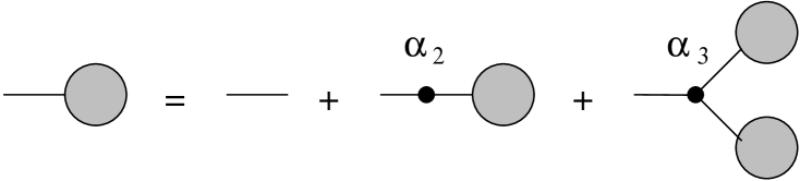
Figure 7: The branched polymer equation that generates percolation clusters.

$${}{{\mathcal{Z}}}=z(1+\alpha_{2}{{\mathcal{Z}}}+\alpha_{3}{{\mathcal{Z}}}^{2})$$ (119)

where $\alpha_{3}=1$ but $\alpha_{2}=2$ and $z$ is the bond occupation probability in PC language. This modified branched polymer ensemble still has $\gamma_{str}={1\over 2}$ and hence, according to our discussion above, $d_{S}={4\over 3}$; in fact it is the simplest extension of ${\mathcal{B}}$. Because of our interest in quantum gravity we defined $d_{S}$ in terms of probabilities averaged over all clusters of size $N$ rather than in terms of a particular “typical” cluster. The calculation picks out the leading non-analyticity as $y\to 1$ after taking the thermodynamic limit; we have (67)

$${}\lim_{N\to\infty}\Phi(1-y,N)\simeq\frac{1}{(1-y)^{1-d_{S}/2}}=\frac{1}{(1-y)^{1/3}}$$ (120)

This shows that in the thermodynamic limit a finite proportion of the $T_{N}$ clusters of size $N$ have $d_{S}={4\over 3}$. As we discussed in section 4.3 clusters with $d_{S}$ smaller than ${4\over 3}$ are present but the number of such clusters is suppressed by a power of $N$ relative to $T_{N}$ and so the probability that they appear as an infinite percolation cluster is zero.

T.J. would like to thank Bergfinnur Durhuus for many helpful discussions. This work was supported in part by PPARC visiting fellowship grant GR/K95086 and by EU grant ERBCHRX CT930343.

Appendix

In this appendix we prove that the GCE generating function (39) with the pole term at $y=1$ removed has an asymptotic expansion about $y=1$.

The return probability $P_{{\mathrm{B}}}(t)$ on an individual polymer B can be expressed in terms of a transfer matrix $T_{{\mathrm{B}}}=1-D_{{\mathrm{B}}}$ where $D_{{\mathrm{B}}}$ is the Laplacian on B. $D_{{\mathrm{B}}}$ has eigenvalues $\{\lambda_{{\mathrm{B}}}^{i},\;i=1\ldots N_{{\mathrm{B}}}\}$; one eigenvalue, $\lambda_{{\mathrm{B}}}^{N_{{\mathrm{B}}}}$, is zero while the rest satisfy $1\geq\lambda_{{\mathrm{B}}}^{i}>0$. We have

$${}P_{{\mathrm{B}}}(t)=\sum_{i=1}^{{N_{{\mathrm{B}}}}}a^{i}_{{\mathrm{B}}}(1-\lambda_{{\mathrm{B}}}^{i})^{t}$$ (121)

where the constants $a^{i}_{{\mathrm{B}}}$ depend on the eigenvectors of $D_{{\mathrm{B}}}$ and satisfy $0\leq a^{i}_{{\mathrm{B}}}\leq 1$. Substituting (121) into (39) but omitting the zero eigenvalue (which generates the pole at $y=1$) we obtain

$${}{{\mathcal{Q}}}^{\prime}(z,y)=\sum_{{\mathrm{B}}\in{\mathcal{B}}}z^{N_{{\mathrm{B}}}}\sum_{t=0}^{\infty}y^{t}\sum_{i=1}^{{N_{{\mathrm{B}}}-1}}a^{i}_{{\mathrm{B}}}(1-\lambda_{{\mathrm{B}}}^{i})^{t}.$$ (122)

${{\mathcal{Q}}}^{\prime}$ is absolutely convergent for $0\leq y<1$, $0\leq z<{1\over 4}$. Using the binomial expansion we get

$$\delta{{\mathcal{Q}}}^{\prime}(z,y) = {{\mathcal{Q}}}^{\prime}(z,y)-{{\mathcal{Q}}}^{\prime}(z,1)$$ (123)

$$= \sum_{{\mathrm{B}}\in{\mathcal{B}}}z^{N_{{\mathrm{B}}}}\sum_{t=0}^{\infty}\sum_{n=1}^{t}{t\choose n}(y-1)^{n}\sum_{i=1}^{{N_{{\mathrm{B}}}-1}}a^{i}_{{\mathrm{B}}}(1-\lambda_{{\mathrm{B}}}^{i})^{t}.$$

The term $(y-1)^{n}$ can be replaced using the integral representation

$${}x^{n}=\frac{1}{\Gamma(n)}\int_{0}^{\infty}v^{n-1}e^{-\frac{v}{x}}\,dv$$ (124)

so that, by re-arranging and re-summing over $n$ and $t$, we get

$${}\delta{{\mathcal{Q}}}^{\prime}(z,y)=\int_{0}^{\infty}\beta(v)\,e^{-\frac{v}{1-y}}\,dv$$ (125)

where

$${}\beta(v)=-\sum_{{\mathrm{B}}\in{\mathcal{B}}}z^{N_{{\mathrm{B}}}}\sum_{i=1}^{{N_{{\mathrm{B}}}-1}}a^{i}_{{\mathrm{B}}}\frac{(1-\lambda_{{\mathrm{B}}}^{i})}{(\lambda_{{\mathrm{B}}}^{i})^{2}}\exp\left(-v\frac{1-\lambda_{{\mathrm{B}}}^{i}}{\lambda_{{\mathrm{B}}}^{i}}\right).$$ (126)

We can now use (125) to develop a formal series in powers of $(1-y)$ by repeatedly integrating by parts which gives

$${}{{\mathcal{Q}}}^{\prime}(z,y)={{\mathcal{Q}}}^{\prime}(z,1)+(1-y)\beta(0)+(1-y)^{2}\beta^{\prime}(0)+\ldots+(1-y)^{n}\beta^{(n-1)}(0)+R_{n}$$ (127)

where

$${}R_{n}=(1-y)^{n}\int_{0}^{\infty}\beta^{(n)}(v)\,e^{-\frac{v}{1-y}}\,dv.$$ (128)

To compute the $n$th derivative of $\beta(v)$ from (126) is trivial and so is the remaining $v$ integral in (128) (remember that $y<1$). We find the remainder term

$${}R_{n}=(1-y)^{n}(-1)^{n+1}\sum_{{\mathrm{B}}\in{\mathcal{B}}}z^{N_{{\mathrm{B}}}}\sum_{i=1}^{{N_{{\mathrm{B}}}-1}}a^{i}_{{\mathrm{B}}}\frac{(1-\lambda_{{\mathrm{B}}}^{i})^{n+1}(\lambda_{{\mathrm{B}}}^{i})^{-n-2}}{\frac{1}{1-y}+\frac{1-\lambda_{{\mathrm{B}}}^{i}}{\lambda_{{\mathrm{B}}}^{i}}}$$ (129)

and the coefficient

$${}\beta^{(n)}(0)=(-1)^{n+1}\sum_{{\mathrm{B}}\in{\mathcal{B}}}z^{N_{{\mathrm{B}}}}\sum_{i=1}^{{N_{{\mathrm{B}}}-1}}a^{i}_{{\mathrm{B}}}{(1-\lambda_{{\mathrm{B}}}^{i})^{n+1}(\lambda_{{\mathrm{B}}}^{i})^{-n-2}}.$$ (130)

We see immediately that

$${}R_{n}=(1-y)^{n+1}(-1)^{n+1}r_{n}$$ (131)

where

$${}r_{n}<\beta^{(n)}(0).$$ (132)

It follows that, provided the $\beta^{(n)}(0)$ exist, the series will be at worst asymptotic.

Letting $\lambda_{{\mathrm{B}}}^{min}$ be the smallest non-zero eigenvalue and using the bound $a^{i}_{{\mathrm{B}}}\leq 1$ we find that

$${}|\beta^{(n)}(0)|<\sum_{{\mathrm{B}}\in{\mathcal{B}}}z^{N_{{\mathrm{B}}}}N_{{\mathrm{B}}}(\lambda_{{\mathrm{B}}}^{min})^{-n-2}.$$ (133)

Now $\lambda_{{\mathrm{B}}}^{min}\sim N_{{\mathrm{B}}}^{-\delta}$ where the largest value taken by $\delta$ is $\delta=2$ (the value for the linear polymer). This leaves us with an upper bound on $\beta^{n}(0)$ of the form

$${}\Gamma(2n+{\textstyle\frac{9}{2}})(1-4z)^{-2n-9/2}.$$ (134)

Of course this is a substantial over-estimate compared to the detailed calculation presented in the body of this paper but it tells us two things. Firstly the series (127) is asymptotic. Secondly, since the linear polymer is only exponentially suppressed in the ensemble, $\beta^{n}(0)$ must grow much faster than $\Gamma(n)$ and hence the series cannot be Borel summable.

References

-
[1]
H.Kawai, N.Kawamoto, T.Mogami and Y.Watabiki,
Phys. Lett. B306 (1993) 19;
Y.Watabiki, Nucl. Phys. B441 (1995) 119;
N.Ishibashi and H.Kawai, Phys. Lett. B322 (1994) 67;
M.Fukuma, N.Ishibashi, H.Kawai and M.Ninomiya, Nucl. Phys. B427 (1994) 139. - [2] J.Ambjørn and Y.Watabiki, Nucl. Phys. B445 (1995) 129.
- [3] S.Catterall, G.Thorleifsson, M.J.Bowick and V.John, Phys. Lett. B354 (1995) 58.
- [4] M.J.Bowick, V.John and G.Thorleifsson, Phys. Lett. B403 (1997) 197.
- [5] J.Ambjørn and K.N.Anagnostopoulos, Nucl. Phys. B497 (1997) 445.
- [6] J.Ambjørn et al, “The quantum space-time of c=-2 gravity”, preprint EPHOU-97-006, NBI-HE-97-19, TIT/HEP-371, hep-lat/9706009.
- [7] J.Ambjørn, J.Jurkiewicz and Y.Watabiki, Nucl. Phys. B454 (1995) 313.
- [8] J.Ambjørn, B.Durhuus and J.Fröhlich, Nucl. Phys. B 257 [FS14](1985) 433.
- [9] V.A.Kazakov, I.K.Kostov and A.A.Migdal, Phys. Lett. 157B (1985) 295.
- [10] F.David, Nucl. Phys. B 257 [FS14](1985) 543.
- [11] J.Ambjørn, B.Durhuus and T.Jonsson, Phys. Lett. B244 (1990) 403.
- [12] B.S. Dewitt, in General Relativity, A Centenary Survey, eds. S.W.Hawking and W.Israel, Cambridge University Press, 1979.
- [13] M.Abramowitz and I.Stegun, Handbook of Mathematical Functions, Dover Publications, 1972.
- [14] F.David, Nucl. Phys. B487 (1997) 633.
- [15] P.Bialas and Z.Burda, Phys. Lett. B384 (1996) 75.
- [16] J.Ambjørn, private communication.
- [17] S.Alexander and R.Orbach, J.Physique Lettres 43 (1982) 625.
- [18] S.Havlin and D.Ben-Avraham, Adv. Phys. 36 (1987) 695.
- [19] F.Leyvraz and H.E.Stanley, Phys. Rev. Lett. 51 (1983) 2048.