A new phase structure in three-dimensional dynamical triangulation model
Abstract
We investigate a new phase structure of the three-dimensional dynamical triangulation model with an additional local term by Monte Carlo simulation. We find that the first order phase transition observed for the naive Einstein-Hilbert action terminates at a finite coefficient of the new term. The phase transition turns into second order at the endpoint, beyond which it becomes a crossover.
1 Introduction
The success of the dynamical triangulation model in two dimensions summarized by its equivalence to the Liouville theory in the continuum limit motivated intensive studies of the model in higher dimensions through Monte Carlo simulation. It turned out, however, that with an action obtained by naive discretization of the Einstein-Hilbert action, the phase transition observed is of first order both in three dimensions and in four dimensions [1]. In lattice theories in general, it is often preferable (e.g. improved actions to reduce the finite lattice spacing effects) or even necessary (e.g. the Wilson term to eliminate doublers) to modify the lattice actions from that obtained by naive discretization of the action in the continuum. We may therefore hope to obtain a second order phase transition in the present case by adding a local term to the naive Einstein-Hilbert action.
The new term we consider is motivated by a possible contribution from the measure for the path integral over the metric and has been first studied in four dimensions [2]. Recently this modified action has been studied in three dimensions by the Monte Carlo renormalization group and a possibility was suggested that the first order phase transition terminates at a finite coefficient of the new term [3] 111Note that our is the minus of the in Ref. [3]. We clarify this possibility by high statistics Monte Carlo simulation using multi-canonical technique.
2 The model
The naive discretization of the Einstein-Hilbert action in the dynamical triangulation model in dimensions gives where and are the number of vertices and simplices respectively in the simplicial manifold. We modify the action as
| (1) | |||||
| (2) |
where is the new coupling constant, and is the number of simplices that contain the node . The summation in (2) is taken over all the nodes in the manifold. This term [2] can be considered as the contribution from the path integral measure , since can be interpreted as the “local volume”, which corresponds to in the continuum.
In the following we consider the canonical ensemble with fixed given by the partition function :
| (3) | |||||
| (4) |
where the summation in (3) is taken over all possible triangulations of -dimensional sphere that contain -simplices. The is the partition function for fixed , which can be given by
| (5) |
where the summation is now taken over all possible triangulations that contain -simplices and vertices. The details of the numerical simulation will be reported elsewhere [4].
3 End point of the first order phase transition

In order to investigate the phase diagram with the modified action, we measure the microcanonical entropy defined by
| (6) |
from which we calculate the microcanonical inverse temperature by
| (7) |
Precise measurement of the microcanonical entropy near the first order phase transition point is possible by using the multi-canonical technique. This was previously done for the unmodified action with in Ref. [5], and the critical exponents consistent with the first order phase transition have been successfully extracted by the finite-size scaling analysis.
In Fig. 3, we show the microcanonical inverse temperature for several values of . Note that the node distribution is given for each and by and the double peak structure in the node distribution, which is a signal of the first order phase transition, can be probed directly by looking at the microcanonical inverse temperature . The double peaks appear if and only if (i) has both local maximum and local minimum and (ii) is set to a value between the local minimum and the local maximum. One can see that the local minimum and the local maximum observed for [5] merge at , beyond which the becomes a monotonous function of . This suggests that the first order phase transition ceases to exist at , beyond which it becomes a crossover.
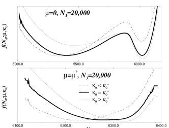
For each below , we define the critical coupling of the phase transition as the position of the peak of the node susceptibility . The end point of the phase transition line is given by for , and for . In Fig. 3, we plot the free energy , which is nothing but the minus log of the node distribution, as a function of near for and . The two local minima observed for merge into one at . The free energy curve at has a wide flat bottom, which suggests the existence of a massless mode.
4 Fractal structure at the end point
In order to examine a possible continuum limit at the end point, we measure the boundary area distribution , which is the number of boundaries with the area at the geodesic distance . The corresponding quantity in two dimensions called the loop length distribution is calculated analytically and is found to possess a continuum limit [6]. The scaling behavior expected from this result has been correctly reproduced by numerical simulation [7].
In Fig. 4, we plot the boundary area distribution at the end point of the first order phase transition line as a function of .

One can see a reasonable scaling behavior. The power of in the scaling variable implies that the fractal dimension is 3. We would like to remark that the scaling behavior we observe is much better than the one that has been claimed to exist with the unmodified action [8].
5 Discussions
Our results suggest that the first order phase transition becomes second order at the end point, where one can obtain a continuous theory. A natural question to be asked is what the continuum theory is. One may suspect that we cannot construct any continuum theory in three-dimensional quantum gravity, since we have no physical degrees of freedom. This argument is too naive, however. An example of field theory which has no physical degrees of freedom that is still completely well-defined is two-dimensional Yang-Mills theory.
The fact that we have to fine-tune two parameters to obtain the continuum limit implies that there are two relevant operators around the fixed point. A possible interpretation of the continuum theory is therefore the gravity. The observation that the fractal dimension at the fixed point is approximately three is also suggestive of this interpretation. The fractal dimension we extracted, however, is still preliminary, and the value might increase as we increase the system size. Needless to say, a lot of work is yet to be done to understand the nature of the continuum theory.
In 4D, the situation is different from the 3D case in that singular vertices which are shared by huge number of -simplices exist in the strong coupling phase [9]. We can add a local term in the action that eliminates these singular vertices, if one wishes, and then the situation becomes more or less the same [4]. We therefore expect that the first order phase transition can be changed into second order by modifying the action.
References
- [1] P. Bialas, Z. Burda, A. Krzywicki and B. Petersson, Nucl. Phys. B472 (1996) 293; B. de Bakker, Phys. Lett. B389 (1996) 238; S. Catteral, R. Renken and J. Kogut, hep-lat/9709007.
- [2] B. Brugmann and E. Marinari, Phys. Lett. B349 (1995) 35.
- [3] R. Renken, Nucl. Phys. B485 (1997) 503.
- [4] T. Hotta, T. Izubuchi and J. Nishimura, in preparation.
- [5] A. Fujitsu and T. Izubuchi, in preparation.
- [6] H. Kawai, N. Kawamoto, T. Mogami and Y. Watabiki, Phys. Lett. B306 (1993) 19.
- [7] N. Tsuda and T. Yukawa, Phys. Lett. B305 (1993) 223.
- [8] H. Hagura, N. Tsuda and T. Yukawa, hep-lat/9512016.
- [9] T. Hotta, T. Izubuchi and J. Nishimura, Prog. Theor. Phys. 94 (1995) 263; S. Catterall, G. Thorleifsson and J. Kogut, Nucl. Phys. B468 (1996) 263.