ITEP-TH-48/97

HUB-EP-97/68

1 Introduction

It might be surprising that topological aspects of the electroweak theory (although being under discussion already for some time outside the lattice community) have not paid due attention to by people doing lattice simulations of the electroweak phase transition. With the present paper, we are entering investigations in that direction for the standard $SU(2)$ Higgs model. The phase transition of this model (without supersymmetric extensions) has lost most of its phenomenological appeal as a viable scenario explaining the generation of baryon asymmetry (taking the present lower limit of the Higgs mass into account). From the non–perturbative point of view in general, this model remains attractive, however, as a laboratory for studying the strong coupling features of high temperature gauge field theory coupled to matter.

In the case of QCD, in contrast to the situation in electroweak theory, the thermal transition between the hadronic and the quark–gluon plasma phase is under intensive study with respect to its topological aspects. The transition is known to be accompanied by a restructuring of the Euclidean field configurations concerning their instanton and monopole content, the latter, however, being detected only by choosing particular gauges. The most promising one in the case of QCD seems to be the maximally Abelian gauge. The Abelian degrees of freedom in this gauge [1] were shown to be relevant for various dynamical properties of the confining phase of Yang–Mills theories realizing the dual superconductor scenario of confinement [2]. This development can be followed in Refs. [3]. The Abelian degrees of freedom provide the dominant contribution to the non-Abelian string tension in the $SU(2)$ gluodynamics [4].

We are wondering whether Abelian monopoles, perhaps in a particular Abelian projection, may also play a non–trivial role in the dynamics of the electroweak theory at high temperature. One outstanding feature of the symmetric phase of the $SU(2)$ fundamental Higgs model is its $3D$ (magnetic) confinement property. Of course, this is also captured in the dimensionally reduced variant of the model which is able to describe the thermal transition with high quantitative accuracy [5]. With respect to $3D$ confinement, the symmetric phase resembles very much the $3D$ pure Yang-Mills theory investigated by Teper [6]. Some years ago, Bornyakov and Grygoryev [7] attempted to identify the agents of confinement in $3D$ pure gauge theory by applying the Abelian projection technique to this model. They found that Abelian monopoles occur with a density becoming constant in the continuum limit $\beta\to\infty$ measured in natural units $g_{3}^{2}=g_{4}^{2}~{}T$. It is known that dimensional reduction cannot describe the nature of the deconfinement transition in QCD. In the electroweak case, however, dimensional reduction has been shown to work very well in the temperature range of interest.

Therefore it seems natural to start our consideration of topological restructuring at the electroweak phase transition by choosing the $3D$ formulation and applying the Abelian projection approach. We will compare the maximally Abelian gauge with a gauge independent prescription which corresponds to Abelian projection from the unitary gauge (for the Higgs field in the fundamental representation). The first approach requires an iterative procedure, and usually the monopole content suffers from gauge dependencies. The second one does not need any gauge fixing.

Instead of addressing directly the phase transition, we will test our tools analyzing certain classical field configurations that exist in the broken phase and are believed to contain pairs of non-Abelian Nambu monopoles [10, 13] (non–Abelian monopolium). Numerical work is in progress [8] indicating that the density of the corresponding type of monopoles to be defined in the present paper indeed behaves almost as an disorder parameter characterizing the $3D$ confining, symmetric phase in the dimensionally reduced theory. The condensation of vortices, presumably the correct order parameter, is presently under study. But if monopole–anti-monopole pairs become unbound in the symmetric phase, being invisibly bound in the broken phase, couldn’t be the monopole separation inside the sphalerons the precursor of this mechanism ?

The sphaleron [9, 10, 11] is believed to be important for the relaxation of an eventual baryon number asymmetry after the electroweak phase transition is completed [12]. In the standard electroweak model all constraints concerning the strength of the electroweak phase transition are derived from the requirement that the thermal barrier factor $exp(-E_{sphal}(T_{c})/T_{c})$ should be sufficiently small to suppress the washing–out of the baryon number in the broken, lower–temperature phase. In the present work we are only interested to learn how the electroweak sphaleron looks like in various Abelian projections. We study the electroweak sphaleron using the $SU(2)$ Higgs model since due to the smallness of the Weinberg angle $\theta_{W}$ the $U(1)$ component of the electroweak group $SU(2)\times U(1)$ has little effect on the sphaleron properties and also the influence of the standard model fermions on the sphaleron solution is quite small. Thus the properties of the sphaleron in the standard electroweak model are basically determined by the $SU(2)$ Higgs sector [12]. The $3D$ sphaleron is perfectly known on the lattice due to the work of Garcia Perez and van Baal [16]. They used a $3D$ variant of the $SU(2)$ fundamental Higgs theory in order to construct sphalerons as saddle point solutions of the lattice energy functional [16].

In the maximally Abelian gauge we find that the sphaleron contains a highly symmetric structure of Abelian monopole–anti-monopole pairs connected by vortex strings. We also study the other definition of defects which corresponds to Abelian projection from the unitary gauge. The sphaleron configurations have been generated just in this gauge [16], but the prescription works without any gauge fixing. We show, that in this Abelian projection the sphaleron contains a Nambu monopole–anti-monopole pair [13] connected by a $Z$-vortex string [10, 13] (non–Abelian monopolium). This result comes not unexpectedly in view of some investigations [14, 15] done in the continuum.

The structure of the paper is as follows. In Section 2 we formulate the maximally Abelian projection of the $SU(2)$ fundamental Higgs model with emphasis on the Higgs degrees of freedom. We show that this model in the maximally Abelian projection contains Abelian monopoles and two types of Abrikosov–Nielsen–Olesen strings [17]. In Section 3 we present our gauge invariant lattice definitions of the Nambu monopole and the $Z$–string. Section 4 is devoted to the analysis of some $3D$ sphaleron configurations (produced by [16]) and Section 5 to the interpretation of our findings.

2 The maximally Abelian Projection of $SU(2)$–Higgs Theory

The maximally Abelian gauge is defined [1] to maximize some gauge–noninvariant functional $R[U]$ by suitable gauge transformations, where $R[U]=\sum_{l}{\rm Tr}\,(U_{l}\sigma^{3}U^{+}_{l}\sigma^{3})$. $U_{l}$ denotes a link representing a $SU(2)$ gauge field and $\sigma^{3}$ is one of the Pauli matrices. The functional $R$ is still invariant under $U(1)$ gauge transformations, $\Omega^{abel}_{x}=e^{i\sigma_{3}\,\alpha_{x}}$, $\alpha_{x}\in[0,2\pi)$. The gauge condition fixes the $SU(2)$ gauge freedom up to the $U(1)$ subgroup.

One speaks about Abelian projection if Abelian link phases $\theta_{l}$ are extracted from the diagonal elements of the $SU(2)$ gauge field $U$ according to $\theta_{l}=\arg U^{11}_{l}\in[-\pi,\pi)$. Usually, the Abelian projection is done after the maximally Abelian gauge has been chosen. Under the residual $U(1)$ gauge transformations the field $\theta_{l}$ behaves as an Abelian gauge field: $\theta_{x,\mu}\to\theta_{x,\mu}+\alpha_{x+\hat{\mu}}-\alpha_{x}$ mod $2\pi$. The components of the $SU(2)$–Higgs field $\Phi={(\phi^{(1)},\phi^{(2)})}^{T}$ transform as follows: $\phi^{(1)}\to e^{i\alpha}\phi^{(1)}$ and $\phi^{(2)}\to e^{-i\alpha}\phi^{(2)}$. Thus the fields $\phi^{(1)}$ and $\phi^{(2)}$ carry Abelian charges $+1$ and $-1$, respectively.

Therefore, the $SU(2)$–Higgs theory in the Abelian projection can be considered as a theory which contains a compact Abelian gauge field $\theta_{l}$ and two charged Abelian $scalar$ fields $\phi^{(1)}$ and $\phi^{(2)}$. The reduced theory possesses two types of topological defects, Abelian monopoles (due to the compactness of the residual Abelian group) and Abelian vortices (due to the presence of the charged scalar fields).

The Abelian plaquette $\theta_{x,\mu\nu}=\theta_{x,\mu}+\theta_{x+\hat{\mu},\nu}-\theta_{x+\hat{\nu},\mu}-\theta_{x,\nu}$ can be decomposed into two parts: $\theta_{x,\mu\nu}={\bar{\theta}}_{x,\mu\nu}+2\pi m_{x,\mu\nu}$. Here ${\bar{\theta}}_{x,\mu\nu}\in[-\pi,\pi)$ is the electromagnetic flux through the plaquette $P_{x,\mu\nu}$ and $m_{x,\mu\nu}$ is an integer associated with a Dirac string. The Abelian monopole charge inside a cube $C$ is identified as follows [18]:

$$j_{C}={(\mbox{d}m)}_{P}\equiv\sum_{P\in\partial C}m_{P}\,,$$ (1)

where the summation is taken over the plaquettes which form the boundary of the cube $C$ and d denotes the lattice differential.

Actually, the effective Abelian theory possesses two types of Abelian vortices since there are two Abelian charged fields. The vorticity numbers (of sort $i$) $\sigma^{(i)}$ carried by the plaquette $P_{x,\mu\nu}$ are given by the following equations [19]:

$$\sigma^{(i)}_{x,\mu\nu}=m_{x,\mu\nu}-l^{(i)}_{x,\mu\nu}\,,\quad l^{(i)}_{x,\mu\nu}=l^{(i)}_{x,\mu}+l^{(i)}_{x+\hat{\mu},\nu}-l^{(i)}_{x+\hat{\nu},\mu}-l^{(i)}_{x,\nu}\,,\quad i=1,2\,,$$ (2)

where the integer-valued link variables $l^{(i)}$ are defined, in terms of the link angles $\theta_{x,\mu}$ and the phases of the respective (upper or lower) Higgs field components $\varphi^{(i)}_{x}=\arg\phi^{(i)}_{x}$, through the usual decomposition

$$\mp\varphi^{(i)}_{x}+\theta_{x,\mu}\pm\varphi^{(i)}_{x+\hat{\mu}}-2\pi l^{(i)}_{x,\mu}\in[-\pi,\pi)\,,\qquad i=1,2\,.$$ (3)

The vorticity number $\sigma^{(i)}_{P}$ is equal to the number of type-$i$ vortices penetrating the plaquette $P$. The vortex trajectories are defined as the set of oriented links which are dual to the plaquettes with non–zero vorticity number. On can check that the Abelian vortices of both types end on the Abelian monopoles, i. e. $\mbox{d}\sigma^{(i)}=j$.

3 The Nambu Monopoles and the $Z$–Strings

There is a gauge invariant and quantized lattice definition of another type of magnetic excitations of the $SU(2)$ Higgs theory, the Nambu monopole [13]. We define a composite adjoint unit vector field $n^{a}_{x}$ by

$$n^{a}_{x}=-\frac{\left(\Phi^{+}_{x},\sigma^{a}\Phi_{x}\right)}{\left(\Phi^{+}_{x},\Phi_{x}\right)}\,,\qquad n_{x}=n^{a}_{x}\,\sigma^{a}\,.$$ (4)

In the following definition of the Nambu monopole the field $n_{x}$ plays a role similar to the direction of the adjoint Higgs field in the definition of the ’t Hooft–Polyakov monopole [20] in the Georgi–Glashow model.

The most transparent definition of the Nambu monopole can be given in the unitary gauge $\Phi={(0,\phi)}^{T}$ ($n^{a}\equiv\delta^{a3}$), where $\phi$ is some complex–valued scalar. This gauge condition leaves Abelian transformations $\Omega^{u}_{x}=e^{-i\sigma^{3}\alpha_{x}}$ free, with $\alpha_{x}\in[0,2\,\pi)$. The superscript ^u refers to the unitary gauge. The phase $\theta^{u}_{l}=\arg U^{11}_{l}$ of some link behaves as a compact $U(1)$ gauge field with respect to the residual Abelian gauge group: $\theta^{u}_{x,\mu}\to\theta^{u}_{x,\mu}+\alpha_{x+\hat{\mu}}-\alpha_{x}\,\,{\rm mod}\,2\pi$. In the continuum $SU(2)$ Higgs theory [13] the $Z$–magnetic flux coincides in the unitary gauge with the Abelian magnetic flux of the field $\theta^{u}_{l}$. Therefore, in the unitary gauge the Nambu monopoles can be identified with the Abelian magnetic defects in the field $\theta^{u}_{l}$.

Now the usual DeGrand–Toussaint construction [18] can be applied to the field $\theta^{u}_{l}$ in order to define the $Z$–charge of the Nambu monopole inside a three-dimensional cube $C$:

$$j^{u}_{C}=\sum_{P\in\partial C}m^{u}_{P}\equiv-\frac{1}{2\pi}\sum_{P\in\partial C}{\bar{\theta}}^{u}_{P}\,,\quad{\bar{\theta}}^{u}_{x,\mu\nu}=\theta^{u}_{x,\mu\nu}-2\pi m^{u}_{x,\mu\nu}\in[-\pi,\pi)\,,$$ (5)

where the summation is taken over the plaquettes which form the boundary of the cube $C$.

There is, however, a gauge invariant way to define the flux ${\bar{\theta}}^{u}_{P}$ which proceeds as follows. First a new set of links $V_{l}$ depending on $U_{l}$ and $n_{x}$ is introduced by the following construction

$$V_{x,\mu}(U,n)=U_{x,\mu}+n_{x}U_{x,\mu}n_{x+\hat{\mu}}\,.$$ (6)

Under general gauge transformations, $V_{l}$ links transform like $U_{l}$ links. They intertwine the adjoint field $n_{x}$ between neighboring places,

$$n_{x}V_{x,\mu}=V_{x,\mu}n_{x+\hat{\mu}}.$$ (7)

Before the fluxes of the $V_{l}$’s are evaluated the new links have to be normalized to $SU(2)$ giving

$$A_{x,\mu}(U,n)=\frac{V_{x,\mu}(U,n)}{\sqrt{\frac{1}{2}{\rm Tr}\Bigl{[}V^{+}_{x,\mu}(U,n)\,V_{x,\mu}(U,n)\Bigr{]}}}\,.$$ (8)

The gauge invariant flux ${\bar{\theta}}^{u}_{P}$ is now calculable as

$${\bar{\theta}}^{u}_{x,\mu\nu}(U,n)=\arg\Bigl{(}{\bf Tr}\left[({\mathchoice{\rm 1\mskip-4.0mul}{\rm 1\mskip-4.0mul}{\rm 1\mskip-4.5mul}{\rm 1\mskip-5.0mul}}+n_{x})A_{x,\mu}A_{x+\hat{\mu},\nu}A^{+}_{x+\hat{\nu},\mu}A^{+}_{x,\nu}\right]\Bigr{)}\,.$$ (9)

The Abelian plaquette (9) is a gauge invariant object because the field $A_{l}$ transforms as an $SU(2)$ link field and the vector $n^{a}_{x}$ as an adjoint matter field. In the unitary gauge, when $n\equiv\sigma^{3}$, the field $A_{l}$ is exactly diagonal

$$A_{x,\mu}(U,\sigma^{3})={\rm diag}\,(e^{i\theta^{u}_{x,\mu}}\,,\,e^{-i\theta^{u}_{x,\mu}})\,,\qquad\theta^{u}_{x,\mu}={\rm arg}U^{11}_{x,\mu}$$ (10)

due to cancellations in (6). Because of (7) the Abelian plaquette is independent of which corner is chosen in order to project the non–Abelian plaquette onto $n_{x}$. The formulae (4-9) give the gauge–invariant lattice definition of the Nambu monopole.

The lattice $Z$–string is primarily defined in the unitary gauge, $\Phi={(0,\phi)}^{T}$. Under the residual Abelian gauge transformations the field $\phi_{x}$ behaves as follows: $\phi_{x}\to e^{i\alpha_{x}}\phi_{x}$. Therefore in the unitary gauge the lower component $\phi_{x}$ of the doublet Higgs field $\Phi_{x}$ has unit electric charge with respect to the Abelian gauge field $\theta^{u}_{l}$. The $Z$–string [10, 13] can be considered as the Abrikosov–Nielsen–Olesen vortex solution [17] embedded [22, 14] into the electroweak theory. As long as we are in the unitary gauge the $Z$–strings can be detected as the vortex topological defects in the Abelian matter field $\phi_{x}$. Then the $Z$-vorticity number through the plaquette $P_{x,\mu\nu}$ can be defined as follows:

$$\sigma^{u}_{x,\mu\nu}=m^{u}_{x,\mu\nu}-l^{u}_{x,\mu\nu}\equiv-\frac{1}{2\pi}\Bigl{(}{\bar{\theta}}^{u}_{x,\mu\nu}-\chi^{u}_{x,\mu\nu}\Bigr{)}\,,$$ (11)

where the link variables $l^{u}_{l}$ and $\chi^{u}_{l}$ are the result of the decomposition

$$\chi^{u}_{x,\mu}=\varphi^{u}_{x}+\theta^{u}_{x,\mu}-\varphi^{u}_{x+\hat{\mu}}-2\pi l^{u}_{x,\mu}\in[-\pi,\pi)\,,\qquad\varphi^{u}_{x}=\arg\phi_{x}\,.$$ (12)

Finally, the non–integer part is used to evaluate the plaquette field $\chi_{x,\mu\nu}\equiv{(\mbox{d}\chi)}_{x,\mu\nu}$. But there is an alternative, gauge independent way to define the field $\chi^{u}_{l}$ as follows:

$$\chi^{u}_{x,\mu}=-\arg\left(\Phi^{+}_{x},A_{x,\mu}\Phi_{x+\hat{\mu}}\right)\,,$$ (13)

where the link field $A_{l}$ is defined in (8). $Z$–vortices begin and end on Nambu (anti-)monopoles: $\mbox{d}\sigma^{u}=j^{u}$. Equations (11-13) comprehend the gauge invariant lattice definition of the $Z$–vortex.

4 Topological Content of Sphaleron: A Few Exercises with Lattices Sphaleron Configurations

The electroweak sphaleron (at Weinberg angle $\theta_{W}=0$) is a saddle point solution of the static equations of motion of the $SU(2)$–Higgs theory. We have studied four three–dimensional electroweak sphaleron configurations which have been originally obtained in Refs. [16] on a $16^{3}$ lattice (with periodic boundary conditions). The sphalerons were prepared by a saddle point cooling algorithm, i.e. cooling with respect to an action which expresses the square of the equation of motion (as written on the lattice). For details, one should consult Refs. [16]. The four sphaleron configurations differ from each other by the physical size of the lattice, $LM_{W}=4$ and $LM_{W}=4.8$, and by different Higgs mass parameters of the model, $M_{H}=M_{W}$ and $M_{H}=0.75~{}M_{W}$. The configurations have been kindly provided to us by the authors of Refs. [16].

First, we observe that the sphaleron configurations happen to be Abelian to a high degree in the (quasi–unitary) gauge they are produced in, $\Phi={(\phi,0)}^{T}$ with $\phi_{x}$ real–valued. The volume average of the sum of the squared diagonal elements in the $SU(2)$ link matrices $U_{l}$ is not less than $0.96$. If the Abelian link angles are extracted in this not yet maximally Abelian gauge, the Nambu $M\overline{M}$ structure hidden in the core of the sphaleron can immediately made visible in the appearance of Abelian monopoles. Nambu monopoles are Abelian monopoles in the (quasi-) unitary gauge. All four sphalerons have the Nambu monopole $M$ and the Nambu anti-monopole $\overline{M}$ at a distance of two lattice spacings at the same place in the lattice. This similarity can be explained by the fact that all sphaleron solutions are derived from a single one by adapting the parameters for the new saddle-point cooling [23]. We relate our observation to the result obtained in the framework of continuum field theory [14, 15] that the sphaleron should contain a pair of Nambu monopole and anti–monopole connected by a piece of $Z$–vortex.

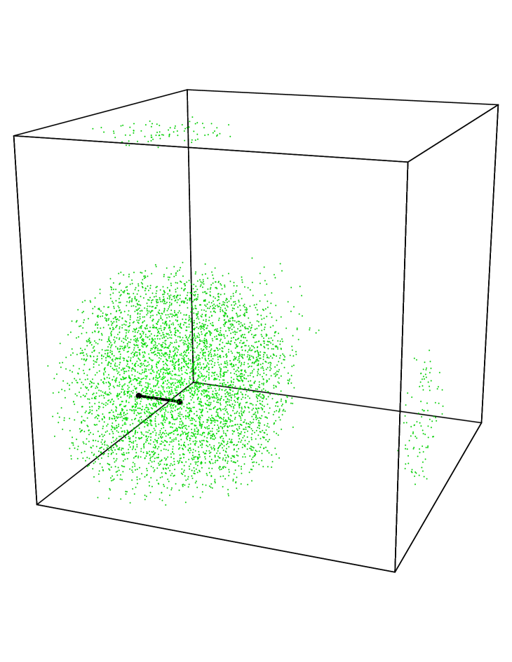
Figure 1: Nambu monopole-anti-monopole pair with Z-vortex in between (non-Abelian monopolium) inside the lattice sphaleron. The positions are the same for all four sphaleron configurations.

The same picture is reproduced by the gauge invariant measuring routine outlined above. The configuration is visualized in Fig. 1. The big points denote the Nambu monopole and anti-monopole, the line in between is the $Z$–vortex trajectory and the volume occupied by the sphaleron is marked by the cloud of small points. Their density is inversely proportional to the modulus of the scalar field. Regions where the length of the scalar field is bigger than $0.75$ are not shown.

After looking into each sphaleron in the quasi–unitary gauge $\Phi={(\phi,0)}^{T}$ with $\phi_{x}$ real–valued, we attempted to put them into the maximally Abelian gauge. This has been done with the standard algorithm adapted to $3D$. There is always an obstruction to reach full Abelianicity. We have searched for the maximum of the gauge-fixing functional $R[U]$ over 100 random gauge copies (to control possible Gribov copies) of each original sphaleron configuration. Our stopping criterion for the gauge cooling iterations was that we continue to cool if the volume minimum of the trace of the local gauge transformation, $1/2\,{\rm Tr}g_{x}$ is less than $1-10^{-8}$. It is remarkable that, for each Gribov copy, at the end of the gauge cooling always one of the Abelian monopole pairs we detected was identical with the Nambu $M\overline{M}$ pair. As the gauge cooling proceeds, few additional pairs of Abelian monopoles pop up and disappear while the Nambu monopole pair always remains among the Abelian monopoles.

Finally put into the maximally Abelian gauge, all investigated sphaleron configurations have Abelian monopoles forming a rotationally invariant (under the cubic group) configuration in the very center of the sphaleron.

For the Higgs mass being equal to the $W$ mass the Abelian monopolium structure is shown in Fig. 2. Now, the big points denote the Abelian monopoles and anti-monopoles and the lines are Abelian vortex trajectories. Figs. 2(a,b) represent the configuration enclosed in the smaller lattice volume. In particular, Fig. 2(a) shows the type-1 vortices and Fig. 2(b) the type-2 vortices. Similarly, in Figs. 2(c,d) we visualize the sphaleron that has been created in the physically larger volume. At the chosen mass ratio there is apparently no volume dependence.

The sphalerons with the mass ratio $M_{H}/M_{W}=0.75$ look somewhat different as can be seen in Fig. 3. In Figs. 3(a,b) the configuration enclosed in the smaller lattice volume is depicted, one time showing the type-1 and the other time the type-2 vortices. Analogously, Figs. 3(c,d) allow to have a look into the sphaleron in the larger lattice volume. Again, the lattice volume plays no important role for the structure of the core. The comparison with Fig 2. suggests that there is an effect of the Higgs mass on the distribution of vortices. In the case of higher Higgs mass there are long vortex trajectories sweeping out in a random walk through the region of high energy density. No such long vortex trajectories are detected in Fig. 3.

5 Conclusion

The fundamental $SU(2)$–Higgs model in $3D$ can be topologically analyzed in terms of Abelian monopoles, for instance in the symmetric phase where these should be related to the $3D$–confining properties. The dimensionally reduced high temperature Higgs theory has a string tension of approximately the same strength as the pure $3D$ gauge theory. The Abelian reduction of the Higgs model from the maximally Abelian gauge leaves two Abelian Higgs fields (with charge $1$ and $-1$ with respect to the $U(1)$ subgroup). Correspondingly, there exist two types of Abelian vortices, which are closed or connect a monopole with an anti–monopole.

In this paper gauge independent lattice definitions of non–Abelian monopoles and vortices (the Nambu monopoles and the $Z$–vortices) have been formulated which describe embedded, topologically unstable defects within the fundamental Higgs model. The Nambu monopole current is topologically conserved in $4D$. The new kind of monopole is identical with the normal Abelian monopole iff the Abelian projection (which leads to the latter) is done in the unitary gauge, but they are still strongly correlated if (as usual) the maximally Abelian gauge is chosen.

There are ideas expressed in the literature [14, 15] that the sphaleron saddle point configuration, from the $3D$ point of view, should consists of a pair of Nambu monopoles stretched along a $Z$-vortex string. We have analyzed a few lattice sphaleron configurations looking from the two perspectives explained above, in terms of Abelian monopoles and vortices on one hand and of non–Abelian Nambu monopoles and $Z$–vortices on the other. This analysis has covered Higgs masses $M_{H}/M_{W}=1.0$ and $0.75$ and volumes ranging from $VM_{W}^{3}=4.0^{3}$ to $4.8^{3}$ on a $16^{3}$ lattice. Since the lattice saddle point configurations have been provided in the quasi–unitary gauge $\Phi={(\phi,0)}^{T}$ with $\phi_{x}$ real–valued, the two pictures are identical for the original sphalerons. There is always just one Nambu monopolium in the center of the sphaleron separated by a distance $d=2a$.

In fact, the original configurations proved to be already relatively Abelian, but then gauge cooling has been applied to put them into the maximally Abelian gauge. In this gauge an Abelian multi–(anti)monopole configuration appears which is maximally symmetric under the cubic rotation group. One of the Abelian monopole–anti-monopole pairs is identical with the non–Abelian Nambu $M\overline{M}$ pair. As the result of gauge cooling, this structure is found for all $O(100)$ random gauge copies per sphalerons that we have prepared to start from. The exact trajectories of the Abelian vortices in the ’maximally’ Abelian gauge differs from copy to copy. Mostly they are of length $2a$. Our results are indicative for an effect that the Higgs mass has on the distribution of the Abelian vortices. In the case of higher Higgs mass there is always one vortex (either of type 1 or type 2) of extension (length) greater than $2a$.

Simulations are now under way in order to clarify the dynamical role of the topological defects discussed here in the context of the thermal Higgs phase transition [8].

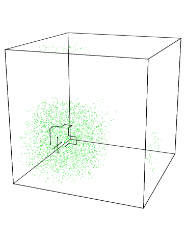
(a)	(b)
(c)	(d)

Figure 2: The sphalerons with $M_{H}=M_{W}$ in the volumes $LM_{W}=4$ (above) and $LM_{W}=4.8$ (below) in the Maximal Abelian gauge with their Abelian monopole content and with Abelian vortices of the type I (left) and the type II (right).

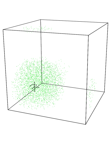
(a)	(b)
(c)	(d)

Figure 3: Same as Figure 2 but for the sphalerons with $M_{H}=0.75~{}M_{W}$.

References

- [1] A. S. Kronfeld et al., Phys. Lett. 198B (1987) 516; A. S. Kronfeld, G. Schierholz and U. J. Wiese, Nucl. Phys. B293 (1987) 461.
- [2] G. ’t Hooft, Nucl. Phys. B190 [FS3] (1981) 455.
- [3] T. Suzuki, Nucl. Phys. B (Proc. Suppl.) 30 (1993) 176; A. Di Giacomo, Nucl. Phys. B (Proc. Suppl.) 47 (1996) 136; M. I. Polikarpov, Nucl. Phys. B (Proc. Suppl.) 53 (1997) 134.
- [4] T. Suzuki and I. Yotsuyanagi, Phys. Rev, D42 (1990) 4257; G. Bali et al., Phys. Rev. D54 (1996) 2863.
- [5] K. Kajantie et al., Nucl. Phys. B466 (1996) 189; M. Gürtler et al., Nucl. Phys. B483 (1997) 383; M. Gürtler, E.-M. Ilgenfritz and A. Schiller, Phys. Rev. D56 (1997) 3888.
- [6] M. Teper, Phys. Lett. B311 (1993) 223.
- [7] V. Bornyakov and R. Grygoryev, Nucl. Phys. B (Proc. Suppl.) 30 (1993) 576.
- [8] M. N. Chernodub, F. V. Gubarev, E.–M. Ilgenfritz and A. Schiller, in preparation.
- [9] R. F. Dashen, B. Hasslacher and A. Neveu, Phys. Rev. D10 (1974) 4138.
- [10] N. S. Manton, Phys. Rev. D28 (1983) 2019.
- [11] F. R. Klinkhamer and N. S. Manton, Phys. Rev. D30 (1984) 2212.
- [12] V. A. Rubakov and M. E. Shaposhnikov, Usp. Fiz. Nauk 166(1996) 493 (Phys. Usp. 39 (1996) 461).
- [13] Y. Nambu, Nucl. Phys. B130 (1977) 505.
- [14] M. Barriola, T. Vachaspati and M. Bucher, Phys. Rev. D50 (1994) 2819.
- [15] M. Hindmarsh and M. James, Phys. Rev. D49 (1994) 6109; M. Hindmarsh, Sintra Electroweak (1994) 195, hep-ph/9408241.
- [16] M. Garcia Perez and P. van Baal, Nucl. Phys. B429 (1994) 451; M. Garcia Perez and P. van Baal, Nucl. Phys. B468 (1996) 277.
- [17] A. A. Abrikosov, Sov. Phys. JETP 32 (1957) 1442; H. B. Nielsen and P. Olesen, Nucl. Phys. B61 (1973) 45.
- [18] T. A. DeGrand and D. Toussaint, Phys. Rev. D22 (1980) 2478.
- [19] M. N. Chernodub, M. I. Polikarpov and M. A. Zubkov, Nucl. Phys. B (Proc.Suppl.) 34 (1994) 256.
- [20] G. ‘t Hooft, Nucl. Phys. B79 (1974) 276; A. M. Polyakov, JETP Lett. 20 (1974) 194.
- [21] V. G. Bornyakov et al., Z. f. Phys. C 42 (1989) 633.
- [22] T. Vachaspati and M. Barriola, Phys. Rev. Lett. 69 (1992) 1867.
- [23] M. Garcia Perez, private communication.