Random Surfaces and Lattice Gravity

Abstract

In this talk I review some of the recent developments in the field of random surfaces and the Dynamical Triangulation approach to simplicial quantum gravity. In two dimensions I focus on the $c=1$ barrier and the fractal dimension of two-dimensional quantum gravity coupled to matter with emphasis on the comparison of analytic predictions and numerical simulations. Next is a survey of the current understanding in 3 and 4 dimensions. This is followed by a discussion of some problems in the statistical mechanics of membranes. Finally I conclude with a list of problems for the future.

1 Outline

There are many approaches to formulating a discrete theory of quantum gravity. In this talk I will focus on the dynamical triangulations (DT) formulation of simplicial gravity. This was first developed in the context of string theory and two-dimensional quantum gravity ($QG_{2}$) where the discrete approach has proven extremely powerful and actually preceded continuum treatments. By now we have considerable confidence in the validity of the assumptions underlying the DT model in the case of coupling of matter with central charge c less than one. This confidence stems from the agreement of discrete, continuum and numerical results.

The situation for central charge c greater than one was clarified in the last year by David [1]. After the Introduction a discussion of this work will be the first part of this review. This is followed by a discussion of recent numerical tests of David’s proposal [2].

I will then move on to the fascinating issue of the intrinsic fractal geometry of $QG_{2}$ and $QG_{2}$ coupled to conformal matter. In any theory of gravity it is natural to ask what effect quantum fluctuations have on the structure of spacetime. The most basic question we could ask of any spacetime with a given topology is: “What is its Hausdorff dimension?” Our current knowledge of the answer to this question will be reviewed, with emphasis on a comparison of analytic predictions with recent numerical simulations.

The success of the DT approach to simplicial gravity in two dimensions has inspired several groups to tackle large scale simulations of the DT discretization of Euclidean Einstein-Hilbert gravity in 3 and 4 dimensions. Here the situation is much cloudier, both theoretically and numerically. The current status will be summarized in the third part of my talk.

Any rich idea usually has many unsuspected spin-offs. The field of random surfaces and non-critical string theory is intimately connected with the physics of membranes. Some recent numerical results on new phases of anisotropic membranes will be discussed as an example of the fascinating interdisciplinary nature of the subject of random surfaces.

Finally I present a list of challenging future problems that I think are essential for progress in the field. I hope that some of them will be solved by the time of Lattice 98.

2 Introduction

String theories may be viewed as 2-dimensional Euclidean quantum field theories with particular actions and matter content. From this viewpoint they may also be considered as 2d-statistical mechanical models on lattices with dynamical geometry. Statistical mechanical models on fixed lattices often possess special critical points where they are scale invariant. Correlation functions of generic matter fields $\Phi(x)$ reflect this scale invariance by transforming very simply under scale transformations: $\langle\Phi\left(\vec{r}\right)\Phi(0)\rangle\sim r^{-2\Delta^{o}_{\Phi}}$, where $\Delta^{o}_{\Phi}$ is the scaling dimension of $\Phi$, or equivalently its anomalous dimension in field theory. Combining scale invariance with locality leads to the much larger symmetry of conformal invariance. In two dimensions conformal invariance and unitarity restrict the possible values of critical exponents because the unitarisable representations of the associated Virasoro algebra form a discrete series parameterized by a single real number — the central charge $c$. The central charge determines the effect of scalar curvature on the free energy of the model [3].

For $c<1$ the only allowed values are

$$c=1-\frac{6}{m(m+1)}\quad\mbox{with}\quad m=2,3,4\ldots$$ (1)

It is also understood, through the classic work of KPZ [4], how scaling dimensions of fields are modified when the lattice becomes dynamical i.e. when the model is coupled to two-dimensional gravity. The dressed scaling dimensions $\Delta_{\Phi}$ are determined solely by $\Delta^{0}_{\Phi}$ and the central charge $c$ via

$$\Delta_{\Phi}-\Delta^{o}_{\Phi}=\frac{\Delta_{\Phi}(1-\Delta_{\Phi})}{1-\gamma_{s}\left(0\right)},$$ (2)

where the string susceptibility exponent $\gamma_{s}$ describes the entropy of random surfaces of fixed area $A$ viz:

$$Z(A)={\rm e}^{\Lambda_{c}A}A^{\gamma_{s}-3}$$ (3)

and

$$\gamma_{s}(h)=2-\frac{1-h}{12}\Big{\{}25-c+\sqrt{(1-c)(25-c)}\,\Big{\}}$$ (4)

for a Riemann surface of genus $h$. Eq.(3) implies the singularity structure

$$Z(\Lambda)=\int^{\infty}_{0}dAe^{-\Lambda A}Z(A)\sim(\Lambda_{c}-\Lambda)^{2-\gamma_{s}}$$ (5)

as $\Lambda\rightarrow\Lambda_{c}$. The renormalized continuum theory is obtained by tuning the cosmological constant $\Lambda$ to the critical cosmological constant $\Lambda_{c}$. In this limit the mean area $\langle A\rangle$ diverges like $1/(\Lambda-\Lambda_{c})$. The linearity of $\gamma_{s}$ with genus $h$ given by Eq.(4) has the remarkable consequence that the partition function including the sum over genus

$$Z(\Lambda,\mu)=\sum^{\infty}_{0}e^{-\mu h}\int^{\infty}_{0}dA\;e^{-\Lambda A}Z(A)$$ (6)

is actually a function not of two variables $\Lambda$ and $\mu$ but only of the single scaling combination

$$x=(\Lambda-\Lambda_{c})\;{\rm exp}\Biggl{[}\frac{\mu}{2}\Biggl{(}1-\sqrt{\frac{1-c}{25-c}}\;\Biggr{)}\Biggr{]}\;.$$ (7)

For the minimal models of Eq.(1) the scaling variable is

$$x=(\Lambda-\Lambda_{c})\;{\rm exp}\Biggl{[}\frac{m}{2m+1}\;\mu\Biggr{]}\;.$$ (8)

The discrete formulation of $QG_{2}$ dates to 1982 and has proven to be even more powerful than the continuum approach [5]. It is very rare in conventional field theories for the discrete formulation to be more flexible than the continuum treatment and the fact that it is so here certainly deserves notice.

In discrete $QG_{2}$ one replaces the 2d-manifold $\Sigma(\xi_{1},\xi_{2})$ by a set of $n$ discrete nodes $\{i\}$ and the metric $g_{ab}(\xi_{1},\xi_{2})$ by the adjacency matrix $C_{ij}$, where $C_{ij}=1$ if $i$ is connected to $j$ and $C_{ij}=0$ otherwise. The connectivity $q_{i}$ of node $i$ is

$$q_{i}=\sum_{j}C_{ij}\;.$$ (9)

The scalar curvature $R_{i}$ is

$$R_{i}=2\pi\frac{6-q_{i}}{q_{i}}\;.$$ (10)

The gravity partition function becomes

$$Z(\Lambda,\mu)=\sum^{\infty}_{0}e^{-\mu h}\sum^{\infty}_{n=0}e^{-\Lambda n}Z_{h,n}\;,$$ (11)

where $Z_{h,n}$ for pure gravity is the number of distinct triangulations (${\cal T}$) of $n$ nodes with genus $h$ and $Z_{h,n}$ for models with matter is symbolically

$$Z_{h,n}=\sum_{{\cal T}}\int{\cal D}[\Phi]e^{-S_{MG}}$$ (12)

for a generic matter field $\Phi$ coupled to gravity with action $S_{MG}$. The density of states $Z_{h,n}$ is best computed by dualizing the triangulation to a $\Phi^{3}$ graph and counting the number of distinct such connected graphs with $n$ vertices that can be drawn, without crossing, on a surface of genus $h$ or greater. To incorporate the topology of the graph one must promote $\Phi$ to an $N\times N$ matrix à la ’t Hooft. The full partition function $Z(\Lambda,\mu)$ is, indeed, simply related to the free energy of the corresponding matrix model:

$$Z(\Lambda,\mu)\equiv\frac{1}{N^{2}}{\rm log}\;\zeta(N,g)\;,$$ (13)

where

$$\zeta(N,g)=\int d^{N^{2}}\Phi\;{\rm exp}[-N\;{\rm Tr}\;(\frac{1}{2}\Phi^{2}-\frac{g}{3}\Phi^{3})]$$ (14)

with the identification

$$\frac{1}{N^{2}}={\rm e}^{-\mu}\quad\mbox{and}\quad g={\rm e}^{-\Lambda}\;.$$ (15)

3 The $c=1$ Barrier

As we have seen in the Introduction there is a good understanding of how scaling dimensions of operators are modified by the coupling of gravity to conformal field theories characterized by a central charge $c$ less than one. In several cases the models are exactly solvable and the sum over topologies is even possible in the double scaling limit $N\rightarrow\infty$ and $\Lambda\rightarrow\Lambda_{c}$ with the scaling variable $x$ of Eq.(7) fixed [6]. When the central charge $c$ exceeds one the string susceptibility exponent $\gamma_{s}$, according to KPZ [4], becomes complex. This unphysical prediction is indicative of an instability in the model. What is the true character of the theory for $c>1$? The $c=1$ point is analogous to the upper critical dimension $d=4$ in the theory of phase transitions and, in fact, there are known logarithmic violations of scaling at c=1 [7].

From numerical simulations for $c>1$ the following picture has emerged. Two basic classes of models have been carefully investigated. The first consists of bosonic matter fields on dynamical triangulations. In these models one finds a branched polymer BP phase for $c$ large (typically $c\geq 5$). The BP phase is characterized by $\gamma_{s}=1/2$ and the proliferation of minimal neck baby universes (mimbus). For smaller values of the central charge ($1<c<4$) the simulations indicate an intermediate phase with $0<\gamma_{s}<1/2$. There is no apparent discontinuity in the vicinity of $c=1$. The second class of models is multiple Ising models on dynamical triangulations. The distinct species of spins couple through the dynamical connectivity of the lattice. For $n$ copies of Ising model there is a spin-ordering transition at a critical temperature. At the critical point one recovers a $c=n/2$ conformal field theory. For $n>2$, but not too large, $\gamma_{s}$ increases smoothly from $0$ to $1/2$ with, again, no discontinuity near $n=2$ ($c=1$). For large $n$ the ordered and disordered spin phases (both with pure gravity exponents $\gamma_{s}=-1/2$) are separated by an intermediate BP phase with $\gamma_{s}=1/2$ and vanishing magnetization. The transition from the magnetized pure gravity phase to the disordered BP phase is a branching transition with $\gamma_{s}=1/2$. This branching is one sign of the expected instability discussed above. Similar phenomena are found for the q-state Potts model for q large. A plot of $\gamma_{s}$ as a function of the central charge $c$ from existing simulations for two classes of triangulations (degenerate ${\cal T_{D}}$ and combinatorial ${\cal T_{C}}$) is shown in Fig.1.

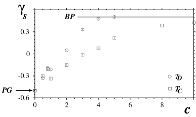
Figure 1: $\gamma_{s}$ vs c for both degenerate ${\cal T_{D}}$ and combinatorial ${\cal T_{C}}$ triangulations.

Could there be a nontrivial infrared fixed point governing the critical properties of the $c\geq 1$ models? A renormalization group scheme for matrix models, roughly analogous to the $\epsilon$-expansion about the upper critical dimension, was developed sometime ago by Brézin and Zinn-Justin (BZ) [8]. A typical example is given by the $2^{n}$-matrix model formulation of the $n$-Ising spins coupled to gravity. The BZ technique consists of integrating out one row and one column of the matrix to obtain an $N-1$ dimensional matrix. Changing $N$ is equivalent to changing the string coupling constant $e^{-\mu}$ of Eq.(15). This induces a flow in the matrix model coupling which leads to definite renormalization group flows. One can then look for fixed points. The method is only qualitatively correct for the well-understood case of $c<1$ minimal models but has the advantage it can be extended to $c>1$. What does it tell us about $c>1$?

David’s idea was to apply the BZ scheme to matrix models that include branching interactions. These interactions generate microscopic wormholes that connect two macroscopic pieces of a Riemann surface. The action for such models is given by

$$S_{N}(\Phi)=N\;{\rm Tr}\left(\frac{\Phi^{2}}{2}-g\frac{\Phi^{4}}{4}\right)-\frac{x}{2}{\rm Tr}^{2}\left(\frac{\Phi^{2}}{2}\right)$$ (16)

The trace-squared (gluing) interaction (with coupling $x$) corresponds to branching and is naturally generated at second order in perturbation theory within a renormalization-group framework. Such models were first treated by Das et al. [9]. For pure gravity it was found that increasing the coupling $x$ leads to a new critical point $(g_{c},x_{c})$ in the $(g,x)$–plane separating a large-$x$ BP phase ($\gamma=1/2$) from the pure gravity phase ($\gamma=-1/2$). At the (branching) transition $\gamma_{s}=1/3$. This result extends to the case of the $m-th$ minimal model. In this case the branching critical point has $\gamma_{s}=1/(m+1)$. Applying the BZ RG method to this case David found the RG flows

$$\begin{array}[]{l}\beta_{g}=g-6g{{}^{2}}-2gx\\ \beta_{x}=2x-3x{{}^{2}}-6gx\end{array}$$ (17)

For $c>1$ the only true fixed point is the BP fixed point. But the influence of the $c<1$ fixed points is still felt for $c$ in the neighbourhood of $1$. For $c<1$ the scaling dimension of the field $x$ (corresponding to the renormalized coupling $x$) is positive and wormholes are irrelevant. At $c=1$ the branching interaction is marginal and the matter-gravity fixed point merges with the branching fixed point. For $c>1$ wormholes are relevant and the matter-gravity and branching fixed points become complex conjugate pairs off the real axis. As a result there are exponentially enhanced crossover effects which imply that an exponential fine-tuning of couplings

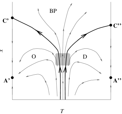
Figure 2: Schematic RG flows for $n>2$ ($c>1$) multiple-Ising models from [1].

$$|g-g{{}_{c}}|\sim{\rm exp}\left(-\frac{1}{\sqrt{c-1}}\right)$$ (18)

is necessary to see the flow to the true BP fixed point. Without this fine-tuning flows appear similar to those for $c<1$. Fig. 2 shows a schematic RG flow for the generalized $n>2$ ($c>1$) multiple-Ising model with branching interactions. In the shaded region flows are similar to the case $c<1$ unless the temperature is fine-tuned. A’ and A” denote pure gravity fixed points and C’ and C” denote branching critical points. The regions $O$ and $D$ are ordered and disordered spin phases respectively. The line $x=0$ corresponds to the original discretized model of $n$-Ising spins on a dynamically triangulated lattice. On this line there is no spin-ordering transition – only the branching transition to the BP phase.

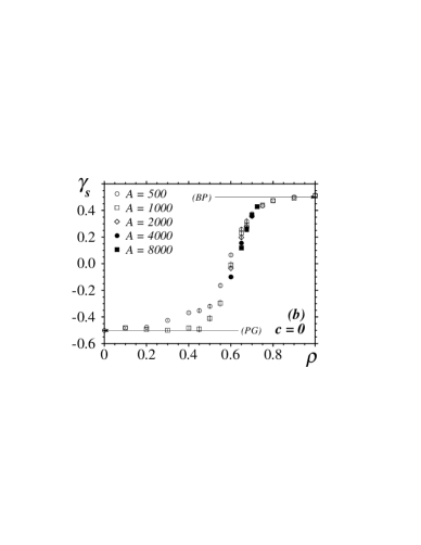
Figure 3: $\gamma_{s}$ vs $\rho$ for $c=0$ from [2].

Figure 4: $\gamma_{s}$ vs $\rho$ for $c=1$ from [2].

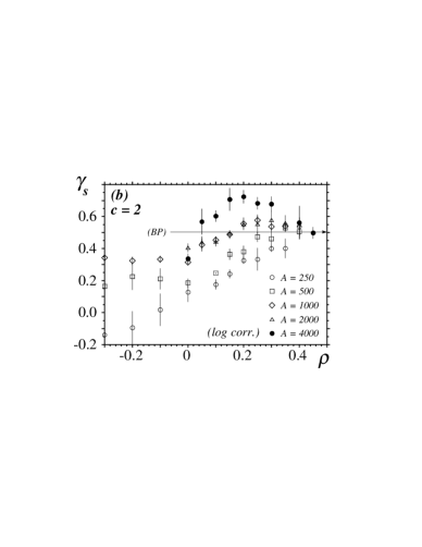
Figure 5: $\gamma_{s}$ vs $\rho$ for $c=2$ from [2].

This nice picture is consistent with the existing numerical results and may also be tested numerically. A first step was reported at this meeting [2]. These authors study the partition function

$$Z_{A}=\sum_{T\epsilon{\cal T}}{\rm e}^{\rho n_{m}}Z_{m}$$ (19)

where $\rho$ is a chemical potential, $n_{m}$ is the number of minimal necks and $Z_{M}$ is a standard matter action for multiple Gaussian fields. The cases studied are zero ($c=0$), one ($c=1$) and two ($c=2$) scalar fields. They look for a transition to the BP phase at a finite critical chemical potential $\rho_{c}$. The clearest results come from an analysis of $\gamma_{s}$ and are shown in Figs. 3–5. For $c=0$ and $c=1$ $\gamma_{s}$ changes sharply from $\gamma\sim-1/2$ to $\gamma\sim 1/2$ at a definite $\rho_{c}$ with $\rho_{c}\sim 0.6$ ($c=0$) and $\rho_{c}\sim 0.4$ ($c=1$). For $c=2$ one finds instead a smooth volume-dependent cross-over to the BP phase. Furthermore the results are consistent with the model being only in the BP phase in the infinite volume limit. These interpretations are supported by an analysis of the specific heat. For $c=0$ and $c=1$ one sees a definite phase transition but for $c=2$ no self-consistent critical exponents can be extracted from finite-size scaling of the specific heat curves.

4 Fractal Dimension

Table 1: The fractal dimension for $c\leq 1$ models: theory and simulations.

$d_{h}$
$c=-2$	$c=0$	$c=1/2$	$c=4/5$	$c=1$	Method
2	4	6	10	$\infty$	Theory: Eq.(23)
3.562	4	4.21	4.42	4.83	Theory: Eq.(24)
3.58(4)	3.58–4.20	3.95–4.35	4.00–4.55	3.8–4.4	Simulations

Our current understanding of the purely spacetime aspects of $QG_{2}$ coupled to matter is much less complete than our knowledge of the effects of gravity on the matter fields and critical behaviour. Of basic interest is the intrinsic Hausdorff dimension of the typical surface appearing in the ensemble of random surfaces. The Hausdorff dimension is defined by

$$d_{H}=\frac{\log A}{\log r}\;,$$ (20)

where $A$ is the area of the surface and $r$ is some appropriate measure of the geodesic size of the surface. There is a considerable variety of alternative definitions of $d_{H}$. In fact $A$ and $r$ here may be replaced by any reparameterization-invariant observables with dimensions of area and distance respectively.

For the case of pure $QG_{2}$ $d_{H}$ is known to be 4 [10, 11]. This result employs a transfer matrix formalism to study the evolution of loops on the surface. One may also use a string field theory for non-critical strings [12] to calculate $d_{H}$. Perhaps the simplest approach is to formulate the theory on a disk with boundary length $\ell$ and to use $\ell$ as a ruler for determining the scaling of both $A$ and $r$. In the string field theory approach an ADM-type gauge is chosen in which geodesic distance plays the role of time. Together with a choice of the string field theory Hamiltonian this determines the scaling of geodesic distance $r$ with boundary length $\ell$ to be

$$r\sim\ell^{1/m}\;,$$ (21)

for the $m-th$ minimal model coupled to $QG_{2}$. The scaling of $A$ vs. $\ell$ may be determined by standard matrix model calculations. If we assume that the area $A$ scales canonically as $\ell^{2}$ we conclude that

$$A\sim r^{2m},$$ (22)

implying $d_{H}=2m$. This result may be equivalently written as

$$d_{H}=\frac{2}{|\gamma_{s}|}=\frac{24}{1-c+{\sqrt{(25-c)(1-c)}}}\;.$$ (23)

A completely different result is obtained by studying the diffusion of a fermion with the methods of Liouville theory [13]. This gives

$$d_{H}=-2\frac{\alpha_{1}}{\alpha_{-1}}=2\times\frac{\sqrt{25-c}+\sqrt{49-c}}{\sqrt{25-c}+{\sqrt{1-c}}}\;,$$ (24)

where $\alpha_{n}$ is the gravitational dressing of a $(n+1,n+1)$ primary spinless conformal field.

In Table 1 we list the predictions from these two formulae together with the results from numerical simulations [14, 15].

Both the analytic predictions discussed above, as well as the exact solution, agree on $d_{H}=4$ for pure $QG_{2}$. A detailed numerical investigation of the fractal dimension, determining both the scaling of two-point functions defined in terms of geodesic distance and the behavior of the loop length distribution function, was presented in this meeting [15]. For $0<c\leq{1}$ $d_{H}$ is found to be very close to 4, in agreement with earlier simulations [14]. An example of the excellent scaling curves obtained is shown in Fig. 6.

Figure 6: Scaling fits for the two point function for $QG_{2}$ from [15].

The current best numerical results therefore do not agree with either of the analytic predictions discussed above. There is not yet complete agreement, to high precision, between the various methods of determining $d_{H}$ and so one cannot confidently rule out both theories. Further work is highly desirable to consolidate the result that $d_{H}$ for $0<c<1$ is independent of the matter. The subtlety of the problem when Ising matter is included may be seen in [16]. The scaling of area versus boundary length depends on the precise order in which the infinite-volume limit is taken with respect to the tuning to the Ising critical temperature. It is possible to obtain $d_{H}=4$ if the infinite-volume thermodynamic limit is taken with $T\neq{T}_{c}$ followed by tuning to the spin-ordering transition. Finally large-scale numerical results for $c=-2$ [17], made possible by recursive sampling of the space of graphs for this topological model, are in excellent agreement with the Liouville prediction $d_{H}=3.56$.

5 Higher Dimensional Simplicial Gravity

Since the DT approach to quantum gravity is very successful in two dimensions it is natural to explore its implications in higher dimensions. There has, in fact, been considerable effort in this direction in recent years. Consider, to begin, the case of pure Einstein-Hilbert gravity in $D$ dimensions for $D=3$ or $4$. The functional integral to be evaluated is

$$Z=\sum_{{\cal M}\in{\rm Top}}\int_{M}\frac{D[g]}{{\rm Vol}({\rm Diff})}\,{\rm e}^{-S(g)},$$ (25)

where $M$ is the spacetime manifold with topology chosen from the class Top and the action $S(g)$ is given by

$$S(g)=\int d^{4}x\;\sqrt{g}\;(\Lambda-\frac{R}{16\pi G}).$$ (26)

In the following we will restrict ourselves to fixed topology since there is little rigorous understanding of the meaning of the sum over of topologies in the general higher dimensional case. The continuum integral over diffeomorphism-inequivalent metrics is replaced in the DT approach by a discrete sum over all possible cellular decompositions (gluings) of $D$-simplices along their $D-1$-faces with the simplicial manifold requirement that the neighbourhood of each vertex is a $D$-ball and the DT constraint that all edge lengths are fixed. So far the majority of numerical results have been limited to the fixed topology of the sphere. To be specific let us concentrate on the $4$-dimensional case of the four-sphere $S^{4}$.

Figure 7: 4d Monte Carlo time history of $N_{0}$ for $N_{4}=64,000$ and $k_{2}=1.278$ from [22]. The horizontal units are 100 sweeps.

Figure 8: Correlation of vertex number $N_{0}$ with singular vertex volume from [23].

The free global variables at our disposal are the numbers $N_{i}({\cal T})$ of $i$-dimensional simplices in a given triangulation ${\cal T}$ ($i=0,1,..,4$). These 5 parameters are constrained by two Dehn-Sommerville relations

$$\sum^{4}_{i=2k-1}(-1)^{i}\pmatrix{i+1\cr 2k-1}N_{i}({\cal T})=0\quad k=1,2$$ (27)

together with the Euler relation

$$\chi\left(S^{4}\right)=\sum_{0}^{4}(-1)^{i}\;N_{i}({\cal T})=2\;.$$ (28)

These three relations leave two independent variables which we may take to be $N_{2}$ and $N_{4}$. These are the discrete analogues of the mean scalar curvature and the volume. The Einstein-Hilbert action Eq.(26) then becomes

$$Z[k_{2},k_{4}]=\sum_{{\cal T}(S^{4})}{\rm exp}[-k_{4}N_{4}({\cal T})+k_{2}N_{2}({\cal T})]$$ (29)

where $k_{4}$ is the discrete cosmological constant and $k_{2}$ is the discrete inverse Newton’s constant. In practice (almost) fixed $N_{4}$ (volume) systems are usually simulated by adding a constraint that restricts the volume to be near a target volume. One is then really approximating the fixed volume partition function

$$Z[k_{2},N_{4}]=\sum_{{\cal T}(S^{4})}{\rm exp}[k_{2}N_{2}({\cal T})]\;.$$ (30)

From extensive numerical simulations it has emerged that the system described by the partition function of Eq.(30) has two distinct phases. For $k_{2}$ small (strong coupling) the system is crumpled (infinite Hausdorff dimension) and the mean scalar curvature $\langle R\rangle$ is negative. For $k_{2}$ large (weak coupling) the system is elongated (branched-polymer like) with Hausdorff dimension 2 and positive mean scalar curvature of order the volume. In the crumpled phase generic triangulations contain one singular one-simplex with two singular vertices [18, 19]. These singular simplices are connected to an extensive fraction of the volume of the simplicial manifold. The local volume associated with the singular one-simplex grows like $V^{2/3}$ while the local volume associated with the singular vertices grows like $V$ itself. The appearance of singular structures is generic to simplicial DT gravity in dimensions $D\geq 4$. For $D\geq 4$ one finds a singular $D-3$ simplex (with local volume of order $V^{2/3}$) and singular sub-simplices (with local volume of order $V$).

It is now clearly established that there is a first order phase transition connecting the crumpled phase with the branched polymer phase in both 3 [20] and 4 dimensions [21, 22]. This is seen dramatically in the time series of Monte Carlo sweeps shown in Fig. 7 [22]. A finite-size scaling analysis of the variance of the $N_{2}$ (or equivalently $N_{0}$) fluctuations also reveals a maximum which grows linearly with the system volume — a classic signal of a first-order transition. It requires both large volumes (order $64,000$) and long simulations (order $10^{6}$ sweeps) to see the first order nature of the transition emerge clearly in four dimensions. It is also becoming clear that the transition itself is closely connected to the formation of the singular simplices [23]. This is demonstrated in Fig. 8.

Many characteristics of the elongated phase are analogous to those of branched-polymers [24] and may be reproduced by simple and elegant statistical mechanical models of branching [25]. With a suitable choice of ensemble this class of models also possesses a discontinuous transition [26]. Thus the weak coupling phase of the theory may reflect more about the combinatorial nature of the simplicial DT action than about the nature of gravity itself. This remains to be seen.

The lack of a continuous transition for DT simplicial gravity in higher dimensions has been a deterrent for recent progress in the field. From a traditional point of view this absence of a critical point implies that the model has no continuum limit we could call continuum quantum gravity. At least three viewpoints are possible at this stage. It may be that the theory is fundamentally discrete and that no continuum limit should be taken. This viewpoint is advocated in different ways in several other approaches to quantum gravity such as the causal sets formulation of Sorkin [27] and the theory of spin networks [28]. Alternatively the theory might only have an interpretation as an effective theory valid over a limited range of length scales. Finally it may be that pure DT simplicial gravity is ill-defined but that models with appropriate matter or modified measures [29] possess critical points and admit a suitable continuum limit. This latter approach was discussed in this meeting by Izubuchi for $QG_{3}$ [30]. One modifies the action by adding terms that effectively enhance higher curvature fluctuations — these correspond to changing the measure locally by powers of $\sqrt{g}$. There is some evidence that by tuning this extra term one can soften the transition to a continuous one at finite volumes. It is very likely though that the effect disappears in the infinite-volume limit. This issue needs further clarification.

6 Membranes

The theory of random surfaces with the addition of an extrinsic curvature to the action has a direct connection with the statistical mechanics of flexible membranes [31]. Physical membranes are two-dimensional surfaces fluctuating in three embedding dimensions. The simplest examples of 2-dimensional surfaces are strictly planar systems called films or monolayers. These alone are surprisingly complex systems. But when they also have the freedom to fluctuate, or bend, in the embedding space it is a considerable challenge to determine their physical properties. Two broad classes of membranes have been extensively studied. Membranes with fixed connectivity (bonds are never broken) are known as crystalline or tethered membranes. Membranes with dynamical connectivity (relatively weak bonds which are free to break and rejoin) are known as fluid membranes.

The simplest action for self-intersecting (non-self-avoiding) fluid membranes resembles that of the Polyakov string with extrinsic curvature (bending energy). Since the beta function for the inverse-bending rigidity (where the bending rigidity is the coupling to the extrinsic curvature) is well-known to be asymptotically free at one loop, the bending rigidity is irrelevant in the infrared and self-intersecting fluid membranes are commonly believed to exist only in a crumpled phase.

Crystalline membranes, on the other hand, have a non-linear coupling between elastic (phonon) interactions and bending fluctuations which drives a phase transition from a high-temperature crumpled phase to a low-temperature orientationally ordered (flat) phase.

Much can be learned about membranes by applying the techniques and experience of lattice gravity simulations to these condensed matter/biological problems. This is illustrated by some recent [32] large-scale Monte Carlo simulations of anisotropic crystalline membranes — these are systems in which the bending or elastic energies are different in different directions. We were able to verify for the first time the predicted existence [33] of a novel tubular phase in this class of membranes. This phase is intermediate between the flat and crumpled phases — it is extended (flat) in one direction but crumpled in the transverse direction. Correspondingly there are two phase transitions: the crumpled-to-tubular transition and the tubular-to-flat transition. Thermalized configurations from the three phases of anisotropic crystalline membranes are shown in Fig. 9. These simulations employed a variety of improved Monte Carlo algorithms such as hybrid overrelaxation and unigrid methods [34]. An even more challenging problem is to incorporate the self-avoidance found in realistic membranes [35, 36].

Figure 9: The three phases of anisotropic membranes:(a) tubular (b) crumpled and (c) flat.

Finally the full physics of fluid membranes, in which dynamical connectivity may be modeled by dynamical triangulations, is a problem of limitless challenges which ties together common techniques in lattice gravity and the burgeoning field of soft condensed matter physics [37].

7 Future Challenges

There are many challenges facing the program of simplicial lattice gravity. I will give here a few outstanding problems and possible future directions.

$\bullet$ Topology Change

Most of the numerical simulations in the field have been on spacetimes with fixed topology. From the functional integral point of view it is more natural (and perhaps essential) to allow the topology of spacetime to fluctuate. In $2d$ it is even possible to perform analytically the sum over all topologies in the double scaling limit. A preliminary investigation of a $4d$ dynamical triangulation model of Euclidean quantum gravity with fluctuating topology was made some time ago by de Bakker [38].

$\bullet$ Supersymmetry

Whether or not it has physical relevance it is clear that one of the most powerful ideas in particle physics/quantum field theory/string theory at present is supersymmetry. Supersymmetry severely constrains the analytic structure of any model. Almost no progress has been made in formulating or simulating supersymmetric simplicial gravity or supersymmetric random surfaces. If we are ever to make contact with critical or non-critical superstrings and recent developments like duality relations this will be essential.

$\bullet$ Classical Limit

Although simplicial quantum gravity does provide a non-perturbative definition of quantum gravity in four dimensions there is no understanding of how classical gravity emerges in the long-wavelength limit and indeed of how perturbative scattering amplitudes are reproduced in this framework.

$\bullet$ Triangulation Class

At present there is no classification of the precise class of graphs that result in KPZ, rather than Onsager, critical exponents when matter is coupled to a dynamical lattice ($QG_{2}$). For example it has been shown [39] that MDT (minimal dynamical triangulation) models in which the local coordination number is restricted to be 5, 6 or 7 still result in KPZ exponents.

$\bullet$ Fractal Dimension

Is the fractal dimension of all $0<c<1$ matter coupled to $QG_{2}$ really four?

$\bullet$ Interpretation of $QG_{4}$

What is the correct interpretation of $4d$ simplicial quantum gravity given the first order transition from the strong to weak coupling phases? What is the proper mathematical framework for $QG_{4}$ and how much analytic progress can be made? Recent progress in this direction is reviewed in [40].

$\bullet$ Renormalization Group

Recently renormalization group (RG) methods have been developed for pure simplicial gravity and for simple matter coupled to gravity [41]. There is no rigorous understanding of the principles behind the success of these methods and further improvement of the technique is highly desirable. Further progress in this direction to enable, for example, the direct computation of the beta function for random surfaces with extrinsic curvature would be very nice.

I would like to acknowledge Kostas Anagnostopoulos, Simon Catterall, Marco Falcioni and Gudmar Thorleifsson for extensive discussion on many issues treated in this talk.

References

- [1] F. David, Nucl. Phys. B487 (1997) 633 (hep-th/9610037).
- [2] G. Thorleifsson and B. Petersson, Beyond the c=1 Barrier in Two-Dimensional Quantum Gravity, to appear in these Proceedings (hep-lat/9709072).
- [3] For a review see P. Ginsparg, Applied Conformal Field Theory, in Fields, Strings and Critical Phenomena, Les Houches 1988, Session XLIX, Eds. E. Brézin and J. Zinn-Justin (North Holland, 1990).
- [4] V.G. Knizhnik, A.M. Polyakov and A.B. Zamolodchikov, Mod. Phys. Lett. A3 (1988) 819.
- [5] D. Weingarten, Nucl. Phys. B210 [FS6] (1982) 229; F. David, Nucl. Phys. B257 (1985) 45; V. A. Kazakov, Phys. Lett. B150 (1985) 28; J. Ambjørn. B. Durhuus and J. Frohlich, Nucl. Phys. B257 (1985) 433; For a review see Quantum Geometry: A Statistical Field Theory Approach, J. Ambjørn, B. Durhuus and T. Jonsson (Cambridge University Press, Cambridge, 1997).
- [6] M. Douglas and S. Shenker, Nucl. Phys. B335 (1990) 635; D. Gross and A. Migdal, Phys. Rev. Lett. 64 (1990) 127; Nucl. Phys. B340 (1990) 333; E. Brézin and V. A. Kazakov, Phys. Lett. B236 (1990) 144.
- [7] I. Klebanov, String Theory in two dimensions, in Proc. Trieste Spring School on String theory and Quantum Gravity 1991 (hep-th/9108019); M. Bowick, M. Falcioni, G. Harris and E. Marinari, Nucl. Phys. B419 [FS] (1994) 665.
- [8] E. Brézin and J. Zinn-Justin, Phys. Lett. B288 (1992) 54.
- [9] S.R. Das, A. Dhar, A.M. Sengupta and S.R. Wadia, Mod. Phys. Lett. A5 (1990) 1041.
- [10] H. Kawai, N. Kawamoto, T. Mogami and Y. Watabiki, Phys. Lett. B306 (1993) 19.
- [11] J. Ambjørn and Y. Watabiki, Nucl. Phys. B445 (1995) 129.
- [12] N. Ishibashi and H. Kawai, Phys. Lett. B314 (1993) 190.
- [13] Y. Watabiki, Progress in Theoretical Physics, Suppl. No. 114 (1993) 1; N. Kawamoto, in Nishinomiya 1992, Proc. eds. K. Kikkawa and M. Ninomiya; in First Asia-Pacific Winter School for Theoretical Physics 1993, Proc. ed. Y.M. Cho.
- [14] S. Catterall, G. Thorleifsson, M. Bowick and V. John, Phys. Lett. B354 (1995) 58; J. Ambjørn, J. Jurkiewicz and Y. Watabiki, Nucl. Phys. B454 (1995) 313; J. Ambjørn, K.N. Anagnostopoulos, U. Magnea and G. Thorleifsson, Phys. Lett. B388 (1996) 713; J. Ambjørn and K.N. Anagnostopoulos, Nucl. Phys. B497 (1997) 445.
- [15] J. Ambjørn, K.N. Anagnostopoulos and G. Thorleifsson, The Quantum Spacetime of 2d Gravity, to appear in these Proceedings (hep-lat/9709025).
- [16] M. Bowick, V. John and G. Thorleifsson, Phys. Lett. B403 (1997) 197 (hep-th/9608030).
- [17] J. Ambjørn, K. N. Anagnostopoulos, T. Ichihara, L. Jensen, N. Kawamoto, Y. Watabiki and K. Yotsuji, Phys. Lett. B397 (1997) 177 (hep-lat/9611032); The quantum space-time of c=-2 gravity (hep-lat/9706009): to appear in Nucl. Phys. B; Intrinsic Geometric Structure of c=-2 Quantum Gravity (hep-lat/9709063):to appear in these Proceedings.
- [18] T. Hotta, T. Izubuchi and J. Nishimura, Prog. Theor. Phys. 94 (1995) 263 (hep-lat/9709073); Nucl. Phys. B. (Proc. Suppl.) 47 (1996) 609.
- [19] S. Catterall, G. Thorleifsson, J. Kogut and R. Renken, Nucl. Phys. B468 (1996) 263.
- [20] J. Ambjørn and S. Varsted, Phys. Lett. B226 (1991) 285; D. Boulatov and A. Krzywicki, Mod. Phys. Lett. A6 (1991) 3003; M. E. Agishtein and A. A. Migdal, Mod. Phys. Lett. A6 (1991) 1863; J. Ambjørn and S. Varsted, Nucl. Phys. B373 (1992) 557; J. Ambjørn, D. Boulatov, A. Krzywicki and S. Varsted, Phys. Lett. B276 (1992) 432; R. L. Renken, S. M. Catterall and J. B. Kogut, Nucl. Phys. B389 (1993) 601; Nucl. Phys. B422 (1994) 677; J. Ambjørn, Z. Burda, J. Jurkiewicz and C. Kristjansen, Phys. Lett. B297 (1992) 253; J. Ambjørn, J. Jurkiewicz, S. Bilke, Z. Burda and B. Petersson, Mod. Phys. Lett. A9 (1994) 2527.
- [21] P. Bialas, Z. Burda, A. Krzywicki and B. Petersson, Nucl. Phys. B472 (1996) 293 (hep-lat/9601024).
- [22] B. de Bakker, Phys. Lett. B389 (1996) 238 (hep-lat/9603024).
- [23] S. Catterall, R. Renken and J. Kogut, Singular Structure in 4D Simplicial Gravity (hep-lat/9709007).
- [24] J. Ambjørn and J. Jurkiewicz, Nucl. Phys. B451 (1995) 643.
- [25] P. Bialas, Z. Burda, B. Petersson and J. Tabaczek, Nucl. Phys. B495 (1997) 463; P. Bialas and Z. Burda, Phys. Lett. B384 (1996) 75; P. Bialas, Z. Burda and D. Johnston, Nucl. Phys. B493 (1997) 505.
- [26] P. Bialas, Z. Burda and D. Johnston, Balls in Boxes and Quantum Gravity (hep-lat/9709056): to appear in these Proceedings.
- [27] R. Sorkin, Forks in the Road to Quantum Gravity, to appear in Int. J. Mod. Phys. A (gr-qc/9706002).
- [28] L. Smolin, The future of spin networks: gr-qc/9702030.
- [29] B. Brugmann and E. Marinari, Phys. Rev. Lett. 70 (1993) 1908.
- [30] T. Hotta, T. Izubuchi and J. Nishimura, A new phase structure in three-dimensional dynamical triangulation model (hep-lat/9710017): to appear in these Proceedings.
- [31] Statistical Mechanics of Membranes and Surfaces, Vol. 5 of the Jerusalem Winter School for Theoretical Physics Proceedings, Eds. D. R. Nelson, T. Piran and S. Weinberg (World Scientific, Singapore, 1989); F. David, in Two Dimensional Quantum Gravity and Random Surfaces, Vol. 8 of the Jerusalem Winter School for Theoretical Physics Proceedings, Eds. D. J. Gross, T. Piran and S. Weinberg (World Scientific, Singapore, 1992); Fluctuating Geometries in Statistical Mechanics and Field Theory, Eds. F. David, P. Ginsparg and J. Zinn-Justin: Les Houches Session LXII (Elsevier Science, The Netherlands, 1996) (http://xxx.lanl.gov/lh94).
- [32] M. Bowick, M. Falcioni and G. Thorleifsson, Phys. Rev. Lett. 79 (1997) 885 (cond-mat/9705059).
- [33] L. Radzihovsky and J. Toner, Phys. Rev. Lett. 75 (1995) 4752 (cond-mat/9510172).
- [34] G. Thorleifsson and M. Falcioni, Improved Algorithms for Simulating Crystalline Membranes: physics/9709026.
- [35] M. Bowick and E. Guitter, Effects of Self-Avoidance on the Tubular Phase of Anisotropic Membranes, to appear in Phys. Rev. E. (1997) (cond-mat/9705045).
- [36] L. Radzihovsky and J. Toner, Elasticity, Shape Fluctuations and Phase Transitions in the New Tubule Phase of Anisotropic Tethered Membranes: cond-mat/9708046.
- [37] T. Lubensky, Solid State Comm. 102 (1997) 187 (cond-mat/9609215).
- [38] B. de Bakker, Nucl. Phys. B (Proc. Suppl.) 42 (1995) 716 (hep-lat/9411032).
- [39] M. Bowick, S. Catterall and G. Thorleifsson, Phys. Lett. B391 (1997) 305 (hep-lat/9605167); Nucl. Phys. B (Proc. Suppl.) 53 (1997) 753 (hep-lat/9608076).
- [40] J. Ambjørn, M. Carfora and A. Marzuoli, The Geometry of Dynamical Triangulations, to appear in Lecture Notes in Physics (hep-th/9612069).
- [41] R. Renken, Phys. Rev. D50 (1994) 5130; R. Renken, S. Catterall and J. Kogut, Phys. Lett. B345 (1995) 422; D. Johnston, J. P. Kownacki and A. Krzywicki, Nucl.Phys. B (Proc.Suppl.) 42 (1995) 728; Z. Burda, J. P. Kownacki and A. Krzywicki, Phys. Lett. B356 (1995) 466; G. Thorleifsson and S. Catterall, Nucl. Phys. B461 (1996) 350; R. Renken, Nucl. Phys. B (Proc. Suppl.) 53 (1997) 783; R. Renken, Nucl. Phys. B485 (1997) 503.