HUB–EP–97/66
September 19, 1997
Topology without cooling: instantons and monopoles
near to deconfinement

Abstract

In an attempt to describe the change of topological structure of pure $SU(2)$ gauge theory near deconfinement a renormalization group inspired method is tested. Instead of cooling, blocking and subsequent inverse blocking is applied to Monte Carlo configurations to capture topological features at a well-defined scale. We check that this procedure largely conserves long range physics like string tension. UV fluctuations and lattice artefacts are removed which otherwise spoil topological charge density and Abelian monopole currents. We report the behaviour of topological susceptibility and monopole current densities across the deconfinement transition and relate the two faces of topology to each other. First results of a cluster analysis are described.

1 INTRODUCTION

An important ingredient of the construction of perfect actions [1] is inverse blocking. This method gives smooth interpolations of background lattice gauge fields on finer and finer lattices which are free of quantum fluctuations. Exploring the topological structure of lattice gauge vacua (and thermal states) requires such an interpolation. It is well-known that some smoothing is needed just to determine the global topological charge in an unambiguous way [2]. Cooling has been proposed iteratively transforming Monte Carlo (MC) configurations into smoother ones by unconstrained relaxation w.r.t. to some action. Due to the diffusive character of cooling it is hard to predict after how many iterations cooled fields exhibit structures characteristic for the quantum ensemble at a definite scale. A random walk estimate asserts that $n$ cooling iterations will keep structures intact at distance $\frac{r}{a}\simeq\sqrt{n}$. Relying on this, cooling is used e. g. to measure the connected field strength correlator at intermediate distances [3]. There are attempts to improve cooling by use of improved actions [4] (measuring with improved topological density) including extended Wilson loops. This can protect instantons at a scale of a few lattice spacing, but still instanton-antiinstanton pairs annihilate at some stage of improved cooling.

Inverse blocking captures topological structure near to the scale of the original lattice spacing by a strictly local procedure. Thus, perfect actions prove their diagnostic power based on the renormalization group. DeGrand et al.[5] demonstrated that one step of inverse blocking suffices to define a perfect total topological charge even if one deals with instantons with $\rho$ not bigger than the lattice spacing. This result has inspired us to examine further the capability of inverse blocking. Our aim was to detect more details of topological structure in terms of topological charge density and monopole currents and to study how they change at the deconfining transition [6].

2 FIXED POINT ACTION AND
INVERSE BLOCKING

We have used a truncated fixed point action with plaquettes and tilted $3$-dimensional $6$-link loops in various representations [5, 6]

$$S_{FP}(U)=\sum_{type~{}i}\sum_{C_{i}}\sum_{j=1}^{4}w(i,j)(1-{1\over 2}~{}{\mathrm{t}r}~{}U_{C_{i}})^{j}.$$ (1)

The lattice size was $L_{s}=12$ and $L_{t}=4$ where simulations have been carried out at $\beta=1.40$, $1.50$, $1.54$, $1.60$ and $1.80$. This interval encloses $\beta_{c}=1.575(10)$ [5] where the deconfinement transition happens for $L_{t}=4$. Our finite temperature results presented below are based on $300$ MC (unsmoothed) configurations and $100$ smoothed ones per $\beta$ value.

Given a coarse configuration with links $V$, inverse blocking gives the constrained minimum of the fixed point action as a configuration $U$ on the next finer lattice. The constraint is formulated including a blocking kernel $T(U,V)$ into the full action functional to be minimized

$$S_{full}(U,V)~{}=~{}S_{FP}(U)~{}+~{}\kappa~{}T(U,V).$$ (2)

Classical perfectness requires saturation

$$\mbox{Min}_{U}(S_{full}(U,V))~{}=~{}S_{FP}(V).$$ (3)

We found this saturation to be fulfilled for equilibrium configurations with an accuracy of a few percent (depending on $\beta$) using an effective $\kappa=5.15$. We convinced ourselves that the physical results to be presented do not very much depend on this parameter.

With a perfect action it should not matter at which level the MC code is actually running. We have simulated on the fine lattice creating links $U$, blocked them to coarse lattice links $V$. Keeping $V$ fixed, by inverse blocking (IB) we obtained $U_{smooth}$, the smoothest interpolation to $V$. Although the final analysis is done on the fine lattice, structures that are resolved belong to the coarse lattice. Being of non–perturbative, long range origin, a confining potential should survive the smoothing step as far as no structures below the coarse level contribute to the string tension. Contrary to this, big changes of topological and monopole densities are expected since quantum fluctuations and dislocations (otherwise counted on the fine lattice) are washed out by smoothing.

3 DOES THE STRING TENSION
SURVIVE SMOOTHING ?

For calibration of the finite temperature lattices for the set of $\beta$ values we have measured the zero temperature string tension on a symmetric lattice $12^{4}$. We have considered temporal, spatially fuzzy Wilson loops and extracted the string tension from fits to the potential energy. We have found a window of approximate scaling around $\beta_{c}$. The two–loop expression for $a(\beta)\Lambda_{L}$ has been used, giving $\sigma/\Lambda_{L}^{2}$ from data for $\sigma a^{2}$ (see table 1).

$\beta$	$1.50$	$1.54$	$1.60$
MC	$135(2)$	$129(2)$	$111(2)$
IB	$100.5(10)$	$104.5(20)$	$96.8(20)$

Table 1: String tension $\sigma/\Lambda_{L}^{2}$ at $T=0$ from fuzzy Wilson loops on a $12^{4}$ lattice

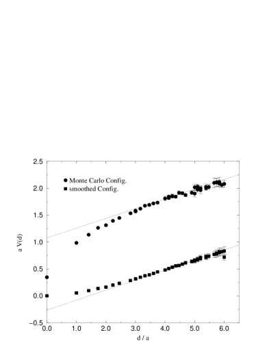
Figure 1: $\overline{q}q$ potential from Polyakov line correlators for MC (above) and smoothed (IB) configurations at $\beta=1.5$

From $75$ to $90$ per cent (with increasing $\beta$) of the $T=0$ string tension are preserved after smoothing. The loss has to be attributed to confining excitations smaller than the spacing $2a$ of the coarse lattice.

A similar effect on the string tension $\sigma(T)$ is observed (see table 2).

$\beta$	$1.50$	$1.54$
$T/T_{c}$	$0.834$	$0.919$
MC	$110(4)$	$118(4)$
IB	$104(2)$	$92(2)$

Table 2: String tension $\sigma(T)/\Lambda_{L}^{2}$ from Polyakov line correlators at two temperatures below $T_{c}$

In Fig. 1 the logarithm of the Polyakov line correlator $\langle L({\bf 0})L({\bf x})\rangle\propto\exp(-V_{\overline{q}q}({\bf x})/T)$ is shown for $\beta=1.5$ where $V_{\overline{q}q}({\bf x})\sim\sigma(T)|{\bf x}|$ at large distances. With short range quantum fluctuations present in the MC configurations, $V_{\overline{q}q}({\bf x})$ contains also the Coulomb potential. As expected, the latter is removed by smoothing while the string tension $\sigma(T)$ is moderately reduced (by less than $5$ per cent at $T<0.8~{}T_{c}$). Very near to the deconfinement temperature, the string tension becomes weaker if measured on smoothed configurations.

4 TOPOLOGICAL VS. MONOPOLE
DENSITY

Monopole currents $m_{\mu}(x)$ are detected in the Abelian projection of $SU(2)$ gauge configurations after these have been put into the maximally Abelian gauge. We reconstruct the topological charge density calculating the local contributions to Lüscher’s geometrical charge and the naive (plaquette oriented) definition of Pontryagin density. Thus we could cross-check both definitions. For MC configurations, the topological charge density is obscured by short range quantum fluctuations and dislocations in both cases. Concerning number and locations of monopole currents the situation is similar. Evaluating the correlator between $|q(x)|$ (of the gauge invariant topological density) and the (gauge dependent !) monopole density $|m_{\mu}(x)|$ fluctuations are averaged out such that no smoothing is required. This was observed earlier for MC configurations generated with Wilson action [7].

Figure 2: Normalized correlation between monopole and topological density at $\beta=1.5$ for MC and smoothed configurations

We show in Fig. 2 the (normalized) correlator comparing MC configurations generated with the fixed point action at $\beta=1.5$ (confinement phase) with the corresponding ensemble of smoothed configurations where the correlator is slightly wider. The same correlation functions at $\beta=1.8$ in the deconfined phase (not shown here), are found to be the same within error bars. The pointlike Abelian monopoles seem to be accompanied by a cloud of topological density, irrespective of the phase. The size of this cloud changes proportional to $1/T$. This correlation is present in MC configurations and in their smoothed counterparts.

Figure 3: Ratio between timelike monopole number $\langle M_{t}\rangle$ and topological activity $\langle A_{top}\rangle$ vs. $T/T_{c}$ for MC and smoothed configurations

Figure 4: Asymmetry between timelike and spacelike monopole currents vs. $T/T_{c}$ for MC and smoothed configurations

This observation suggests that a global relation exists between the topological activity $A_{top}=\sum_{x}|q(x)|$ and the number of monopole currents $M_{\mu}=\sum_{x}|m_{\mu}(x)|$, almost independent of smoothing and phase. Although both quantities are strongly reduced by smoothing, the ratio of averages does not change very much and remains a smooth function of temperature. This becomes even clearer if one considers only the temporal monopole current $M_{t}$, as Fig. 3 demonstrates. In view of the different role timelike ($M_{t}=M_{4}$) and spacelike monopole currents play for confinement (for magnetic confinement above $T_{c}$), the ratio between $M_{s}=\sum_{1}^{3}M_{\mu}$ and $3~{}M_{t}$ is expected to be an disorder parameter of the deconfinement transition [8]. The high monopole activity in MC configurations hides this while smoothing makes it visible, as the comparison in Fig. 4 demonstrates.

5 TOPOLOGICAL SUSCEPTIBILITY

The topological susceptibility is defined here by the fluctuation of topological charge per configuration, $\chi=\langle Q^{2}\rangle/(N_{sites}~{}a^{4})$, with charges $Q$ according to the naive and Lüscher’s topological charge density. For MC configurations the two charges are almost uncorrelated in contrast to smoothed ones.

Figure 5: Lüscher’s vs. naive topological charge for smoothed configurations at $\beta=1.5$

$\beta$	$T/T_{c}$	$\chi^{(l)}/\Lambda_{L}^{4}$	$\chi^{(n)}/\Lambda_{L}^{4}$
$1.50$	$0.834$	$.287(24)10^{4}$	$.370(27)10^{2}$
$1.54$	$0.919$	$.310(27)10^{4}$	$.449(43)10^{2}$
$1.61$	$1.089$	$.235(19)10^{4}$	$.753(59)10^{2}$
$1.80$	$1.732$	$.190(16)10^{4}$	$.308(24)10^{3}$
$1.50$	$0.834$	$.358(47)10^{3}$	$.240(29)10^{3}$
$1.54$	$0.919$	$.324(43)10^{3}$	$.239(30)10^{3}$
$1.61$	$1.089$	$.138(25)10^{3}$	$.962(18)10^{2}$
$1.80$	$1.732$	$.164(11)10^{2}$	$.100(70)10^{2}$

Table 3: Topological susceptibilities of the MC (above) and smoothed (below) samples

Fig. 5 shows a corresponding scatter plot. From the slope we can extract a renormalization factor $Z_{q}(\beta)$ of the naive charge for smoothed configurations, $Z_{q}~{}q(x)~{}a^{4}=q_{naive}(x)~{}a^{4}$. In the neighbourhood of the phase transition we obtained $Z_{q}=0.826$, $.877$ and $.843$ for $\beta=1.50$, $1.54$ and $1.61$, respectively.

Susceptibility data for MC and smoothed configurations (still without renormalization of the naive topological charge) are given in table 3. $\chi^{(l)}$ (based on Lüscher’s geometric charge) is reduced by smoothing by one to two orders of magnitude (going from confinement to deconfinement). This means that the fixed point action does not sufficiently suppress topological dislocations. They are smoothed away by blocking and inverse blocking. This is in accordance to the observation [5] that a sensible measurement of topological charge (even a geometrical one) requires interpolation by inverse blocking.

The naive topological density has a perturbative $Z_{q}<<1$ for $SU(2)$ Wilson action in the relevant $\beta$ range. Also with the fixed point action used for production of MC configurations, the naive topological susceptibility $\chi^{(n)}$ (without proper renormalization) is two orders of magnitude lower than $\chi^{(l)}$ defined through (integer valued) charges if calculated for MC configurations. After smoothing, however, the susceptibilities $\chi^{(n)}$ and $\chi^{(l)}$ do not differ by more than $30$ per cent. This difference can be accounted for by the effective renormalization factor defined above for smoothed configurations. A unique $\chi$ emerges whose $\beta$-dependence is turned into $T$-dependence in Fig. 6. For definiteness, the lattice spacing has been expressed through the zero temperature string tension measured for each $\beta$, respectively, on the symmetric lattice. To normalize we can assume a string tension $\sigma=(440\mbox{MeV})^{2}$ and obtain a susceptibility $\chi=(165.5\mbox{MeV})^{4}$ at $T=0.834~{}T_{c}$.

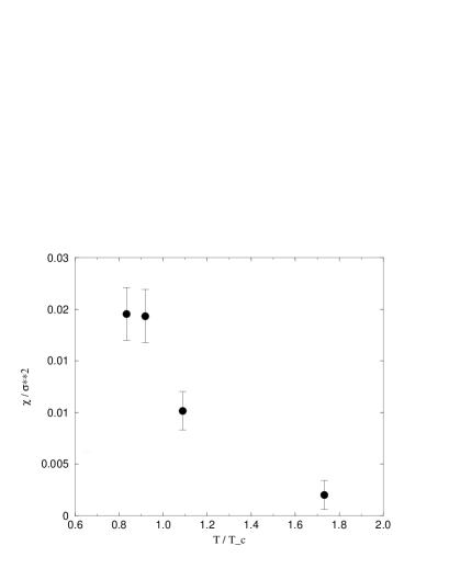
Figure 6: Topological susceptibility for smoothed configurations vs. $T/T_{c}$

6 ARE INSTANTONS BUILDING THE
TOPOLOGICAL SUSCEPTIBILITY ?

A non-trivial two-point correlator of topological density is difficult to obtain without smoothing. For MC configurations it vanishes at non–zero distance (apart from a negative kinematical signal at $d<2a$). For smoothed configurations, however, the correlator can be described by folding the instanton profile according to a dilute gas picture. An ”instanton radius” $\rho$ can be formally defined in this way. This interpretation should be taken with care. In confinement, this $\rho/a$ is found independent of $\beta$, near to the lowest instanton size detectable by inverse blocking, somewhat smaller than the lattice spacing of the blocked lattice. In deconfinement, $\rho/a$ becomes even smaller with increasing $\beta$.

Instanton models [9] use statistical mechanics arguments to relate the density of instantons and antiinstantons to vacuum energy and topological susceptibility by low energy theorems (as well as to make predictions on the multiplicity distribution). Assumptions on instanton interactions enter into these models which can be checked measuring the average density of instantons independently from the topological susceptibility. A first attempt was to compare $A_{top}$ defined above (this makes sense only for smoothed configurations) with $\chi$. Over the temperature range considered $A_{top}$ decreases, but less rapid than $\chi$ (as can be seen in Fig. 7). The horizontal line is a bound set by

Figure 7: Ratio between $\langle Q^{2}\rangle$ and topological activity $\langle A_{top}\rangle$ of smoothed configurations vs. $T/T_{c}$

a low energy theorem for $T=0$

$$\chi=\frac{6}{11}\frac{\langle A_{top}\rangle}{N_{sites}a^{4}}=\frac{6}{11}\langle n_{+}+n_{-}\rangle.$$ (4)

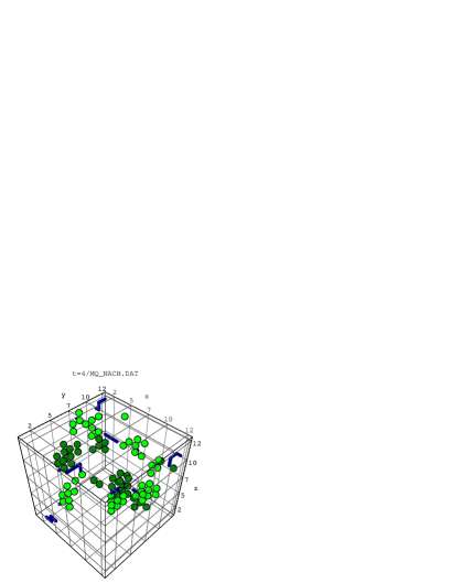
Figure 8: One timeslice of a smoothed configuration: monopole world lines and clusters of topological charge density with $|q^{(l)}(x)|>q_{0}$

The crucial factor $4/b=12/(11N_{c})$ ($b$ is the one–loop coefficient in the $\beta$-function) appears also in the instanton liquid equation of state $\langle N\rangle/V=\langle n_{+}+n_{-}\rangle=(4/b)|\varepsilon_{vac}|$, the width of the multiplicity distribution $\langle N^{2}\rangle-\langle N\rangle^{2}=(4/b)\langle N\rangle$ (compressibility smaller than Poisson) and in the entropic bound $S/(2\pi^{2})>4/b$ (for carriers of charge $Q=1$) banning dislocations. Interactions leading to a $O(1/N_{c})$ suppression of the topological susceptibility compared to the densities $n_{\pm}$ have been discussed [10] in the earliest days of the instanton liquid model.

In fact, $A_{top}$ is only an upper bound for $N$. Further illumination is expected from a cluster analysis of smoothed configurations. A typical example is shown in Fig. 8. But there come surprises: Clusters do not look like classical instantons. The size cannot estimated from the maximum of $|q(x)|$. If isolated charges are removed by few cooling steps, the cluster charges are centered around $Q_{cl}=\pm 1$. Although the mean multiplicity of clusters drops drastically at $T_{c}$, the variance follows Poisson’s law at all temperatures across the transition. We hope to clarify further the nature of the topological composition of the $SU(2)$ vacuum in ongoing work.

References

- [1] T. DeGrand et al., Nucl. Phys. B454 (1995) 587; 615.
- [2] E.-M. Ilgenfritz et al., Nucl. Phys. B168 (1986) 693.
- [3] A. Di Giacomo et al., Nucl. Phys. Proc. Suppl. 54A (1997) 343.
- [4] Ph. de Forcrand et al., Nucl. Phys. B499 (1997) 409.
- [5] T. DeGrand et al., Nucl. Phys. B475 (1996) 321; B478 (1996) 349.
- [6] M. Feurstein et al., hep-lat/9611024
- [7] S. Thurner et al., Phys. Rev. D54 (1996) 3457.
- [8] V. G. Bornyakov et al., Phys. Lett. B284 (1992) 99
- [9] T. Schäfer, E. V. Shuryak, hep-ph/9610451
- [10] E.-M. Ilgenfritz, M. Müller-Preussker, Phys. Lett. B99 (1981) 128