Finite Temperature Quark Confinement via Chromomagnetic Fields

Abstract

A natural mechanism for finite temperature quark confinement arises via the coupling of the adjoint Polyakov loop to the chromomagnetic field. Lattice simulations and analytical results both support this hypothesis. Finite temperature SU(3) lattice simulations show that a large external coupling to the chromomagnetic field restores confinement at temperatures above the normal deconfining temperature. A one-loop calculation of the effective potential for SU(2) gluons in a background field shows that a constant chromomagnetic field can drive the Polyakov loop to confining behavior, and the Polyakov loop can in turn remove the well-known tachyonic mode associated with gluons in an external chromomagnetic field. For abelian background fields, tachyonic modes are necessary for confinement at one loop.

1 INTRODUCTION

The utility of the Polyakov loop ${\cal P}$ makes finite temperature lattice gauge theory a natural place to study confinement. A key issue is the mechanism which drives the Polyakov loop expectation value to zero in the confined phase. In section 2, it is shown that a large external field coupled to $F_{\mu\nu}$ restores confinement above the deconfinement temperature, explicitly demonstrating a connection between the chromomagnetic field and confinement. In section 3, analytical results for $SU(2)$ give a form for the coupling between ${\cal P}$ and $F_{\mu\nu}$.

2 RESTORATION OF CONFINEMENT ABOVE $T_{C}$ BY AN APPLIED EXTERNAL FIELD

An external field $J_{\mu\nu}$ can be coupled to the gauge field $F_{\mu\nu}$ by adding to the lattice action a term of the form

$$\sum_{x}\sum_{\mu>\nu}\sum_{a}{1\over N}\left[J_{\mu\nu}^{a}(x)F_{\mu\nu}^{a}(x)\right]$$ (1)

where the sums are over lattice sites, directions in space-time and directions in the Lie algebra of the gauge group. For the lattice form of the gauge potential, the simplest definition is used:

$$F_{\mu\nu}(x)={1\over 2i}\left[U_{\mu\nu}(x)-U_{\mu\nu}^{+}(x)\right].$$ (2)

For lattice simulations, it is most convenient to not fix the gauge, as would be necessary in the continuum. As a consequence, the partition function $Z$ satifies

$$Z\left[g(x)J_{\mu\nu}(x)g^{+}(x)\right]=Z\left[J_{\mu\nu}(x)\right].$$ (3)

For the case we consider where $J$ is non-zero in a single hyperplane, this property of $Z$ under local gauge transformations implies that $Z$ depends only on the eigenvalues of $J$.

Figure 1 shows the results of simulations of $SU(3)$ lattice gauge theory on a $16^{3}\times 4$ lattice at $\beta=6.0$, plotting the Polyakov loop $P$ against source $J_{12}^{3}$ and $J_{34}^{3}$. The superscript $3$ indicates that the source is in the $\lambda_{3}$ direction in the gauge group, while the subscript indicates sources coupled to $F_{\mu\nu}$ in the $12$ and $34$ direction, thus coupling to the real chromomagnetic field and the imaginary chromoelectric field, respectively. With $J=0$, $\beta=6.0$ at $N_{t}=4$ is well into the deconfined phase of finite temperature $SU(3)$. The phase transition to the confined phase for sufficiently large $J$ is obvious in the figure. Examination of time series and histograms indicate that the transition observed in Figure 1 is most likely first order. A comparison of $J_{12}^{3}$ and $J_{12}^{8}$ shows no evidence for asymmetry in the gauge group: $\lambda_{3}$ and $\lambda_{8}$ appear equivalent. A small difference is seen between $J_{12}^{3}$ and $J_{34}^{3}$, consistent with the more direct connection of the temporal plaquettes to Polyakov loops via the link elements $U_{4}$.

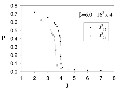
Figure 1: $Tr_{F}({\cal P})$ versus source $J$.

The restoration of symmetry by a sufficiently strong external field coupled to the chromomagnetic field is reminiscent of the restoration of the normal phase from the superconducting phase by a strong magnetic field. It is natural from this point of view to consider the system in a dimensionally reduced form, in which the Polyakov loop play the role of a Higgs field in the adjoint representation, coupled to a three-dimensional gauge field.

A complimentary approach is to view the effect of the external field as changing the effective coupling constant. For the simple case considered here, it is possible to find an alternative form for the action by explicitly integrating over all local gauge transformations. The leading term in $J_{\mu\nu}$ is proportional to $Tr\left[J_{\mu\nu}^{2}\right]Tr\left[F_{\mu\nu}^{2}\right]$, with a negative sign, indicating a reduction in the effective value of the gauge coupling $\beta$.

3 QUARK CONFINEMENT BY CONSTANT FIELDS

One plausible scenario for confinement is that the coupling between the local gauge field $F_{\mu\nu}$ and the adjoint Polyakov loop produces an effective action which leads to two different phases [1]. In the low temperature phase, there is a magnetic condensate and the Polyakov loop indicates confinement; in the high temperature phase the magnetic condensate vanishes, the Polyakov loop indicates deconfinement, and the contribution of the thermal gauge boson gas dominates the free energy. This occurs because finite temperature effects naturally couple the local gauge field to Polyakov loops[2, 3, 4, 5].

For $SU(N)$, the fundamental and adjoint representation Polyakov loops are related by

$$Tr_{A}({\cal P})=|Tr_{F}({\cal P})|^{2}-1.$$ (4)

Clearly, when $Tr_{A}({\cal P})$ assumes its minimum value of $-1$, $Tr_{F}({\cal P})$ assumes the value $0$. Thus, one way to produce confinement in the low temperature phase is for the free energy to be minimized by minimizing the expected value of the trace of the adjoint Polyakov loop.

The case of a constant background chromagnetic field in $SU(2)$ illustrates this possibility. The color magnetic field and the Polyakov loop are taken to be simultaneously diagonal, and the color magnetic field $H$ points in the $x_{3}$ direction. The Polyakov loop is specified by a constant $A_{0}$ field, given in the adjoint representation by $A_{0}=\phi\tau_{3}/{2\beta}$. The trace of the Polyakov loop is then given by $Tr_{F}({\cal P})=2\cos(\phi/2)$ in the fundamental representation and by $Tr_{A}({\cal P})=1+2\cos(\phi)$ in the adjoint representation. The external magnetic field we take to have the form $A_{2}=Hx_{1}\tau_{3}/2$ which gives rise to a chromomagnetic field $F_{12}=H\tau_{3}/2$.

The one-loop contribution to the free energy has the usual form [6, 7, 8] of a sum over the logarithms of modes. The crucial contributions to this mode sum comes from modes of the form

$$\left[\left(\omega_{n}-{\phi\over\beta}\right)^{2}+2H\left(m+{1\over 2}\pm 1\right)+k_{3}^{2}\right]$$ (5)

where the $\omega_{n}=2\pi n/\beta$ are the usual Matsubara frequencies, and where the terms $2H(m+1/2\pm 1)$ are the allowed Landau levels of the gauge field in a background chromomagnetic field.

When $\phi=0$, the $n=0$ and $m=0$ modes give rise to tachyonic modes for $k_{3}$ sufficiently small; these in turn give rise to an imaginary part in the free energy [6]. These same modes will give a strictly real factor to the determinant provided

$$\beta\sqrt{H}<\phi<2\pi-\beta\sqrt{H}.$$ (6)

The renormalized effective potential has real component

$$V_{R} = {11H^{2}\over 48{\pi}^{2}}\,\ln\left({H\over{\mu}_{0}^{2}}\right)-{2\pi^{2}\over 90\beta^{4}}-{(H)^{3/2}\over{\pi}^{2}\beta}\,\cdot$$

$$\quad\sum_{n=1}^{\infty}\,{\cos(n\phi)\over n}\bigg{[}K_{1}(n\beta\sqrt{H})-{\pi\over 2}Y_{1}(n\beta\sqrt{H})$$

$$\quad+2\sum_{m=0}^{\infty}\,\sqrt{2m+3}K_{1}[n\beta\sqrt{(2m+3)H}\,]\bigg{]}$$ (7)

and imaginary component

$$V_{I}=-{H^{2}\over 8\pi}-{H^{3/2}\over 2\pi\beta}\,\sum_{n=1}^{\infty}\,{\cos(n\phi)\over n}\,J_{1}(n\beta\sqrt{H}).$$ (8)

At low temperatures, minimization of $Re(V)$ leads to $\phi=\pi$ being preferred. This is shown in Figure 2, which plots the real part of the effective potential versus $H/\mu^{2}$ at $T/\mu=0.25$ for both $\phi=0$ and $\phi=\pi$. Unfortunately, examination of $V_{I}$ shows that the lowest minima is not stable, lying just to the right of the stable region, so that this background field configuration remains unstable. The confining solution $(\phi=\pi)$ is preferred over the perturbative vacuum only for sufficiently low temperatures. The tachyonic mode is responsible for $\phi=\pi$ being favored at low temperature, and appears in the expression for $V_{R}$ as the $Y_{1}$ term. Analysis shows that, at one loop for an arbitrary abelian background field, tachyonic modes must occur when $\phi=0$ if $\phi=\pi$ is to be favored at low temperature. If there are no tachonic modes, $\phi=0$ is always favored.

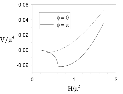
Figure 2: $V/\mu^{4}$ at $T/\mu=0.25$ for $\phi=0$ and $\phi=\pi$.

4 CONCLUSIONS

There is strong evidence from simulations and perturbation theory for the relevance of the chromomagnetic field in confinement, but we are still far from builing a realistic model of the QCD vacuum. Directions for future research along the lines discussed here include simulations and analytical work to determine the effect of a quenched random field $J$ and to explore the behavior of instantons, monopoles and vortices in an external field.

References

- [1] P. N. Meisinger and M. C. Ogilvie, hep-lat/9703009, to be published in Phys. Lett. B.
- [2] P. N. Meisinger and M. C. Ogilvie, Nucl. Phys. B (Proc. Suppl.) 42, 532 (1995).
- [3] P. N. Meisinger and M. C. Ogilvie, Phys. Rev. D 52, 3024 (1995).
- [4] P. N. Meisinger and M. C. Ogilvie, Nucl. Phys. B (Proc. Suppl.) 47, 519 (1996).
- [5] P. N. Meisinger and M. C. Ogilvie, Phys. Lett. B 379, 163 (1996).
- [6] N. K. Nielsen and P. Olesen, Nucl. Phys. B144, 376 (1978).
- [7] M. Ninomiya and N. Sakai, Nucl. Phys. B190 [FS3], 316 (1981).
- [8] P. van Baal, Nucl. Phys. B (Proc. Suppl.) 47, 326 (1996).