DESY 97-188
Non-perturbative quark mass renormalization

Abstract

We show that the renormalization factor relating the renormalization group invariant quark masses to the bare quark masses computed in lattice QCD can be determined non-perturbatively. The calculation is based on an extension of a finite-size technique previously employed to compute the running coupling in quenched QCD. As a by-product we obtain the $\Lambda$–parameter in this theory with completely controlled errors.

1 INTRODUCTION

Calculations of the quark masses in lattice QCD are in principle straightforward, but there are several sources of systematic errors which must be carefully studied (see ref. [1] for a review of the status of these calculations and an up-to-date list of references). One of the uncertainties arises from the renormalization constant needed to convert from the lattice normalizations to the ${\rm\overline{MS\kern-0.50003pt}\kern 0.50003pt}$ scheme of dimensional regularization. Usually one relies on bare perturbation theory (or some modified form thereof) to evaluate this factor. Since only the one-loop term of the expansion is known, and since the gauge coupling is not small on the accessible lattices, the associated error is, however, difficult to estimate. While the extension of the perturbation expansion to the next order may be helpful at this point, it is quite clear that a non-perturbative determination of the renormalization factor will be required to remove all doubts on the reliability of the quark mass calculations in lattice QCD.

The calculation of the quark mass renormalization factor discussed in this talk is based on a recursive finite-size technique which allows one to compute the scale evolution of the renormalized parameters and fields from low to very high energies. An uncontrolled application of perturbation theory can thus be avoided. The general strategy of the computation has already been described in ref. [2] and it is our aim here to report on the progress that has been made along these lines in the case of the quark mass renormalization (for an alternative approach to the problem see refs. [3, 4]).

2 PCAC RELATION

Quark mass ratios can be accurately estimated using chiral perturbation theory (see ref. [5] for a recent discussion). To determine the absolute values of the quark masses in any given renormalization scheme it is hence sufficient to compute a particular linear combination of them such as the sum of the up quark mass and the strange quark mass. A possible starting point then is the PCAC relation

$$\partial_{\mu}(\bar{u}\gamma_{\mu}\gamma_{5}s)_{\rm R}=(\kern 1.0pt\overline{\kern-1.0ptm\kern-1.0pt}\kern 1.0pt_{\rm u}+\kern 1.0pt\overline{\kern-1.0ptm\kern-1.0pt}\kern 1.0pt_{\rm s})(\bar{u}\gamma_{5}s)_{\rm R}$$ (1)

between the renormalized $\Delta S=1$ axial current and the associated renormalized pseudo-scalar density.

In O($a$) improved lattice QCD the axial current and density are given by [6]

$$(\bar{u}\gamma_{\mu}\gamma_{5}s)_{\rm R}=Z_{\rm A}\left(1+b_{\rm A}am_{\rm q}\right)(\bar{u}\gamma_{\mu}\gamma_{5}s)_{{\rm lat}},$$ (2)

$$(\bar{u}\gamma_{5}s)_{\rm R}=Z_{\rm P}\left(1+b_{\rm P}am_{\rm q}\right)(\bar{u}\gamma_{5}s)_{{\rm lat}},$$ (3)

where $(\ldots)_{{\rm lat}}$ denotes the unrenormalized improved fields and $m_{\rm q}$ is the average of the bare $u$ and $s$ quark masses (with the additive renormalization taken into account). Eq. (1) then holds up to terms of order $a^{2}$. In the present context the factors $1+b_{\rm X}am_{\rm q}$ amount to corrections of a few percent at most. The one-loop expression [7]

$$b_{\rm A}-b_{\rm P}=-0.001\times g_{0}^{2}+\ldots$$ (4)

and a recent non-perturbative calculation of this difference [8] moreover suggest that these factors nearly cancel in eq. (1). At the present level of accuracy it thus appears safe to drop them.

So if we determine $(m_{\rm u}+m_{\rm s})_{{\rm lat}}$ through the vacuum-to-kaon matrix element of the unrenormalized PCAC relation,

$$\partial_{\mu}(\bar{u}\gamma_{\mu}\gamma_{5}s)_{{\rm lat}}=(m_{\rm u}+m_{\rm s})_{{\rm lat}}(\bar{u}\gamma_{5}s)_{{\rm lat}},$$ (5)

it follows that

$$\kern 1.0pt\overline{\kern-1.0ptm\kern-1.0pt}\kern 1.0pt_{\rm u}+\kern 1.0pt\overline{\kern-1.0ptm\kern-1.0pt}\kern 1.0pt_{\rm s}=(m_{\rm u}+m_{\rm s})_{{\rm lat}}Z_{\rm A}/Z_{\rm P}.$$ (6)

The calculation of $(m_{\rm u}+m_{\rm s})_{{\rm lat}}$ is standard by now [1] and will not be discussed here. As for the renormalization factors we note that $Z_{\rm A}(g_{0})$ has been computed non-perturbatively [9] to a precision of about $1\%$, using a variant of the chiral Ward identity method of refs. [10]–[14].

The remaining unknown factor in eq. (6) thus is the renormalization constant $Z_{\rm P}(g_{0},a\mu)$. This factor is much harder to determine than $Z_{\rm A}(g_{0})$, because it is a function of two variables, the gauge coupling and the normalization scale $\mu$ of the chosen renormalization scheme.

Figure 1: Scale evolution of the running quark masses in quenched QCD

3 SCALE DEPENDENCE

In the continuum theory the scale evolution of the running coupling and quark masses is governed by the renormalization group equations

$$\mu{\partial\bar{g}\over\partial\mu}=\beta(\bar{g}),\qquad\mu{\partial\kern 1.0pt\overline{\kern-1.0ptm\kern-1.0pt}\kern 1.0pt\over\partial\mu}=\tau(\bar{g})\kern 1.0pt\overline{\kern-1.0ptm\kern-1.0pt}\kern 1.0pt.$$ (7)

For the case of dimensional regularization with minimal subtraction the $\beta$- and $\tau$-functions have been calculated up to 4-loop order of perturbation theory ([15]–[17] and references cited there). Using these results the evolution equations can be integrated starting at some large $\mu$ where the value of the running coupling is known. If we define the renormalization group invariant quark masses $M$ through

$$M=\lim_{\mu\to\infty}\kern 1.0pt\overline{\kern-1.0ptm\kern-1.0pt}\kern 1.0pt\,(2b_{0}\bar{g}^{2})^{-d_{0}/2b_{0}},$$ (8)

where $b_{0}$ and $d_{0}$ are the one-loop coefficients of the $\beta$- and the $\tau$-function respectively, the curves shown in fig. 1 are thus obtained.

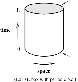
$A_{k}(x)=C^{\prime}_{k}$ $A_{k}(x)=C_{k}$

Figure 2: Space-time manifold used to set up the SF scheme

It should be evident at this point that the knowledge of the running quark masses at high energies is equivalent to providing the values of the corresponding renormalization group invariant quark masses. In other words, instead of $\kern 1.0pt\overline{\kern-1.0ptm\kern-1.0pt}\kern 1.0pt_{\rm u}+\kern 1.0pt\overline{\kern-1.0ptm\kern-1.0pt}\kern 1.0pt_{\rm s}$ we may just as well compute $M_{\rm u}+M_{\rm s}$. It is easy to show that the renormalization group invariant masses are non-perturbatively defined and that they do not depend on the chosen renormalization scheme. We can hence compute them in any scheme that we like such as the one described in the following paragraphs.

4 SF SCHEME

The Schrödinger functional (SF) scheme is a particular finite-volume renormalization scheme which has previously been used to compute the running coupling in the pure SU(3) gauge theory [18]. Its application in the present context has already been discussed in ref. [2] and in this preliminary report we only describe some of the key features of the scheme.

The basic idea is to consider QCD in a finite space-time volume of size $L$ in all directions. Renormalization conditions are then specified at scale $\mu=1/L$ and vanishing quark masses. To be able to perform numerical simulations at zero quark masses the boundary conditions are chosen in such a way that a frequency gap of order $1/L$ is induced on the quark and gluon fields. This can be achieved by assuming the space-time manifold to be as shown in fig. 2 and by imposing Dirichlet boundary conditions at time $x_{0}=0$ and $x_{0}=L$. More precisely, the spatial components of the gauge field are required to be equal to some prescribed constant abelian fields $C$ and $C^{\prime}$. The response of the system to a change of these boundary values may be used to define a running coupling $\bar{g}^{2}$. We do not give any further details here, because the definition of $\bar{g}^{2}$ that we have used is exactly the same as in ref. [18].

Figure 3: Quark diagrams contributing to $f_{\rm P}(z)$ (diagram a) and $f_{1}$ (diagram b). The horizontal lines indicate the boundaries of space-time at $x_{0}=0$ and $x_{0}=L$. The pseudo-scalar density is inserted at the point $z$

The renormalized quark masses in the SF scheme are defined through the PCAC relation and the renormalization condition for the pseudo-scalar density (cf. sect. 2). The precise form of the latter is of only practical importance since all definitions lead to the same values of the renormalization group invariant quark masses. A simple choice for the renormalization constant is

$$Z_{\rm P}(g_{0},L/a)=c\sqrt{f_{1}}/f_{\rm P}(z)|_{z_{0}=L/2},$$ (9)

where $f_{\rm P}(z)$ and $f_{1}$ are unrenormalized correlation functions involving the pseudo-scalar density and the quark fields at the boundaries of space-time [6, 9] ($c$ is to be chosen such that $Z_{\rm P}=1$ at $g_{0}=0$). The corresponding quark diagrams are shown in fig. 3. Note that the renormalization factors associated with the boundary quark fields cancel in the ratio (9). In particular, the renormalized coupling and quark masses defined in this way satisfy the usual renormalization group equations [eq. (7)] with $\mu=1/L$ and the appropriate $\beta$- and $\tau$-functions.

Figure 4: Simulation results for the step scaling function $\sigma(\bar{g}^{2})$ (quenched QCD)

5 RENORMALIZATION GROUP

In the SF scheme a change of the normalization scale amounts to a change of the lattice size at fixed bare parameters. By considering pairs of lattices with sizes $L$ and $2L$, we can thus study the evolution of the running coupling and quark masses under changes of the normalization scale by factors of $2$. The important point to note is that the box size $L$ can be as small as we like in physical units. The only restriction is that $L$ and the low-energy physical scales in the theory (such as the radius $r_{0}$ [19]) should be significantly greater than the lattice spacing to avoid large cutoff effects. Such studies can be carried out using numerical simulations and the scale evolution of the renormalized parameters is thus obtained non-perturbatively.

Close to the continuum limit the evolution from size $L$ to $2L$ is described by the “step scaling functions” $\sigma$ and $\sigma_{\rm P}$ through

$$\bar{g}^{2}(2L)=\sigma(\bar{g}^{2}(L)),$$ (10)

$$Z_{\rm P}(2L)=\sigma_{\rm P}(\bar{g}^{2}(L))Z_{\rm P}(L).$$ (11)

It is our experience that the lattice corrections to these equations are small and can be extrapolated away by repeating the computation of the step scaling functions for various lattice spacings at fixed $\bar{g}^{2}$. The step scaling function associated with the coupling has first been calculated in ref. [18] and further data have since then been added so that this function is now known very accurately over a large range of couplings (see fig. 4). As for the other function, $\sigma_{\rm P}$, the available data (fig. 5) are already quite usable and further runs will be made to fill the gap at large couplings and to achieve a better precision. All these results refer to the continuum limit, i.e. they involve an extrapolation to $a=0$ as indicated above.

Figure 5: Preliminary results for the step scaling function $\sigma_{\rm P}(\bar{g}^{2})$ (quenched QCD)

Once the step scaling functions have been determined, the sequence of couplings and quark masses

$$u_{k}=\bar{g}^{2}(2^{k}L),\qquad m_{k}=\kern 1.0pt\overline{\kern-1.0ptm\kern-1.0pt}\kern 1.0pt(2^{k}L),$$ (12)

is obtained recursively using

$$u_{k+1}=\sigma(u_{k}),\qquad m_{k+1}=m_{k}/\sigma_{\rm P}(u_{k}).$$ (13)

Since $\sigma(u)$ is monotonic the recursion can also be solved backwards, i.e. we can move up and down the energy scale as we wish.

A technical problem here is that the step scaling functions are only known at certain values of the coupling and only to a finite numerical precision. This difficulty can be resolved by fitting the data with a polynomial, as shown in the figures, and using the fit functions in the recursion (13). We have verified that the systematic error which is incurred by this procedure is neglible compared to the statistical errors provided one stays in the range of couplings covered by the data.

6 RESULTS

The largest value of $\bar{g}^{2}$ which can be reached with the available data for the step scaling functions is $3.48$. This corresponds to a certain box size $L_{\rm max}$, which is large enough that contact can be made with the physical low-energy scales in the theory. Following ref. [18], and using some recent results of the UKQCD collaboration [20, 21], one finds $L_{\rm max}/r_{0}=0.680(26)$. This can be taken as initial condition for the non-perturbative evolution of the coupling and the recursion (13) then yields the data points shown in fig. 6. For comparison we also plot the curves that one obtains by integrating the 2- and 3-loop evolution equation starting at the right-most data point. Evidently the exact evolution of the SF coupling is accurately matched by perturbation theory down to surprisingly low energies.

Figure 6: Evolution of the running coupling $\alpha(\mu)=\bar{g}^{2}/4\pi$, $\mu=1/L$, in quenched QCD, taking $r_{0}=0.5$ fm to convert to physical units

We now digress a little bit and discuss how the $\Lambda$-parameter can be extracted from the calculated values of the running coupling. The idea is to evaluate the exact expression

$$\Lambda=\mu(b_{0}\bar{g}^{2})^{-b_{1}/2b_{0}^{2}}{\rm e}^{-1/2b_{0}\bar{g}^{2}}$$

$$\kern 15.00002pt\times\exp\left\{-\int_{0}^{\bar{g}}{\rm d}g\left[{1\over\beta(g)}+{1\over b_{0}g^{3}}-{b_{1}\over b_{0}^{2}g}\right]\right\}$$ (14)

at the high-energy data points of fig. 6. In this range of couplings the integral in the last factor may be reliably calculated using the perturbation expansion of the $\beta$-function, which (in the SF scheme) is now known to 3-loop order [22]. Higher-order corrections are negligible at this point, and after converting to the ${\rm\overline{MS\kern-0.50003pt}\kern 0.50003pt}$ scheme the result

$$\Lambda^{(0)}_{{\rm\overline{MS\kern-0.35002pt}\kern 0.35002pt}}=251\pm 21\,{\rm MeV}$$ (15)

is obtained, where $r_{0}=0.5$ fm has been used to set the scale (the index $\scriptstyle(0)$ reminds us that this number is for quenched QCD).

Figure 7: Evolution of the running quark mass given in units of the renormalization group invariant mass $M$ [eq. (8)]

Now that the evolution of the coupling is under control, it is straightforward to obtain the data points in fig. 7 by solving the quark mass part of the recursion (13). Initially the recursion yields the ratio $\kern 1.0pt\overline{\kern-1.0ptm\kern-1.0pt}\kern 1.0pt(L)/\kern 1.0pt\overline{\kern-1.0ptm\kern-1.0pt}\kern 1.0pt(2L_{\rm max})$. As in the case of the $\Lambda$ parameter, the evolution may then be continued to infinite energy using the 2-loop expression for the $\tau$-function in the SF scheme. In this way one is able to extract the renormalization group invariant mass $M$ and hence the ratio $\kern 1.0pt\overline{\kern-1.0ptm\kern-1.0pt}\kern 1.0pt(L)/M$ plotted in fig. 7. Note that here too the scale evolution is accurately reproduced by perturbation theory down to the lowest energies. In particular, there is little doubt that the use of the perturbative evolution at high energies is safe. We would like to emphasize, however, that the absence of large corrections to the perturbative evolution of the running quark mass depends on the chosen scheme and should not be taken as a general feature of the theory.

At the lowest-energy data point in fig. 7 we have

$$L=2L_{\rm max},\qquad M/\kern 1.0pt\overline{\kern-1.0ptm\kern-1.0pt}\kern 1.0pt=1.18(2).$$ (16)

Recalling our discussion in sects. 2 and 3, it follows from this that the total renormalization factor, relating the bare current quark mass appearing in eq. (5) to the renormalization group invariant mass, is given by

$$M/m_{{\rm lat}}=1.18(2)\times Z_{\rm A}(g_{0})/Z_{\rm P}(g_{0},2L_{\rm max}/a).$$ (17)

The factors $Z_{\rm A}$ and $Z_{\rm P}$ on the right-hand side of this equation are listed in table 1 for two values of the bare coupling $\beta=6/g_{0}^{2}$. Taking the product then yields the desired renormalization factor. These numbers are still preliminary, but they show what can be expected to come out once our study has been completed.

Table 1: Evaluation of eq. (17)

$\beta$	$2L_{\rm max}/a$	$Z_{\rm P}$	$Z_{\rm A}$	$M/m_{{\rm lat}}$
$6.0$	$\phantom{1}9.03(3)$	$0.490(2)$	$0.791(9)$	$1.90(4)$
$6.2$	$11.63(2)$	$0.500(2)$	$0.807(8)$	$1.90(4)$

We finally mention that the one-loop formula

$$M/m_{{\rm lat}}=(2b_{0}g_{0}^{2})^{-4/11}\left\{1-0.12\times g_{0}^{2}+\ldots\right\}$$ (18)

evaluates to $1.81$ and $1.84$ at $\beta=6.0$ and $\beta=6.2$ respectively. This compares quite well with the non-perturbative result quoted in table 1. Note, however, that significantly lower values would be obtained if the expansion was written in terms of Parisi’s boosted bare coupling.

7 CONCLUSIONS

In this work we have demonstrated that scale-dependent renormalization factors can be calculated non-perturbatively without compromising approximations. The methods that we have employed are completely general and are hence expected to be useful in other contexts as well.

Quark mass values are usually quoted in the ${\rm\overline{MS\kern-0.50003pt}\kern 0.50003pt}$ scheme of dimensional regularization at a normalization mass $\mu=1$ GeV or $\mu=2$ GeV. Once a non-perturbative solution of the theory becomes possible, this convention is not entirely satisfactory, because the ${\rm\overline{MS\kern-0.50003pt}\kern 0.50003pt}$ scheme is only meaningful to any finite order of perturbation theory. The renormalization group invariant masses, on the other hand, are non-perturbatively defined and scheme-independent. These quark masses are hence more quotable than the ${\rm\overline{MS\kern-0.50003pt}\kern 0.50003pt}$ masses and we would like to recommend their use in future studies.

Previous computations of the $\Lambda$-parameter in LQCD have shown that this is a rather elusive quantity. The basic problem is that it refers to the high-energy limit of the continuum theory which is not readily accessible on the lattice. Applying our recursive method we have now been able to overcome this difficulty and to obtain the $\Lambda$-parameter with completely controlled errors (apart from quenching which remains to be the major limitation of present-day LQCD).

This work is part of the ALPHA collaboration research programme. We thank DESY for allocating computer time to this project.

References

- [1] T. Bhattacharya and R. Gupta, plenary talk given at the conference
- [2] K. Jansen et al., Phys. Lett. B372 (1996) 275
- [3] G. Martinelli et al., Nucl. Phys. B445 (1995) 81
- [4] L. Giusti (APE collab.), talk given at the conference, hep-lat/9709004
- [5] H. Leutwyler, Phys. Lett. B378 (1996) 313
- [6] M. Lüscher, S. Sint, R. Sommer and P. Weisz, Nucl. Phys. B478 (1996) 365
- [7] S. Sint and P. Weisz, Nucl. Phys. B502 (1997) 251
- [8] G. M. de Divitiis (APETOV collab.), talk given at the conference
- [9] M. Lüscher, S. Sint, R. Sommer and H. Wittig, Nucl. Phys. B491 (1997) 344
- [10] M. Bochicchio et al., Nucl. Phys. B262 (1985) 331
- [11] L. Maiani and G. Martinelli, Phys. Lett. B178 (1986) 265
- [12] G. Martinelli et al., Phys. Lett. B311 (1993) 241, E: B317 (1993) 660
- [13] M. L. Paciello, S. Petrarca, B. Taglienti and A. Vladikas, Phys. Lett. B341 (1994) 187
- [14] D. S. Henty et al., Phys. Rev. D51 (1995) 5323
- [15] T. van Ritbergen, J. A. M. Vermaseren and S. A. Larin, Phys. Lett. B400 (1997) 379
- [16] K. G. Chetyrkin, Phys. Lett. B404 (1997) 161
- [17] J. A. M. Vermaseren, S. A. Larin and T. van Ritbergen, Phys. Lett. B405 (1997) 327
- [18] M. Lüscher, R. Sommer, P. Weisz and U. Wolff, Nucl. Phys. B413 (1994) 481
- [19] R. Sommer, Nucl. Phys. B411 (1994) 839
- [20] H. Wittig (UKQCD collab.), Nucl. Phys. B (Proc. Suppl.) 42 (1995) 288
- [21] H. Wittig (UKQCD collab.), unpublished
- [22] A. Bode, talk given at the conference