D-Theory: Field Theory via Dimensional Reduction of Discrete Variables

Abstract

A new non-perturbative approach to quantum field theory — D-theory — is proposed, in which continuous classical fields are replaced by discrete quantized variables which undergo dimensional reduction. The 2-d classical $O(3)$ model emerges from the $(2+1)$-d quantum Heisenberg model formulated in terms of quantum spins. Dimensional reduction is demonstrated explicitly by simulating correlation lengths up to 350,000 lattice spacings using a loop cluster algorithm. In the framework of D-theory, gauge theories are formulated in terms of quantum links — the gauge analogs of quantum spins. Quantum links are parallel transporter matrices whose elements are non-commuting operators. They can be expressed as bilinears of anticommuting fermion constituents. In quantum link models dimensional reduction to four dimensions occurs, due to the presence of a 5-d Coulomb phase, whose existence is confirmed by detailed simulations using standard lattice gauge theory. Using Shamir’s variant of Kaplan’s fermion proposal, in quantum link QCD quarks appear as edge states of a 5-d slab. This naturally protects their chiral symmetries without fine-tuning. The first efficient cluster algorithm for a gauge theory with a continuous gauge group is formulated for the $U(1)$ quantum link model. Improved estimators for Wilson loops are constructed, and dimensional reduction to ordinary lattice QED is verified numerically.

1 Introduction

The conventional approach to field quantization is to perform a path integral over classical fields. Wilson’s formulation of lattice field theory maintains close contact with perturbation theory by following this approach. This has obvious advantages, for example, in QCD when one wants to make contact with continuum perturbative results. On the other hand, the close relation to perturbative methods may imply that it is unnecessarily difficult to probe the non-perturbative regime. Here we propose an alternative method to quantize field theories. Instead of using continuous classical fields, we work with discrete quantized variables. In scalar field theories these variables are generalized quantum spins, and in gauge theories they are quantum links. It may seem paradoxical that models with continuous symmetries can be expressed using discrete variables. Note, however, that — although a spin $1/2$ has only two discrete states — the continuous $SO(3)$ symmetry is represented exactly. D-theory generalizes this structure to other symmetries.

Why should this quantization procedure be equivalent to performing a path integral over classical fields? A quantum spin operates in a finite Hilbert space. How can the full Hilbert space of a quantum field theory be recovered when the classical fields are replaced by analogs of quantum spins? As we will see, this requires specific dynamics: the dimensional reduction of discrete variables. This dynamics arises in quantum antiferromagnets as well as in quantum link models [1], which are the gauge analogs of quantum spin systems [2, 3]. The dimensional reduction of discrete variables leads to a new non-perturbative D-theory formulation of quantum field theory [4]. Quantized variables can be used e.g. to formulate $O(N)$, $SU(N)\otimes SU(N)$ and $CP(N)$ spin models, as well as Abelian $U(1)$ and non-Abelian $SO(N)$, $SU(N)$, and $U(N)$ gauge theories, in particular, QCD [5].

D-theory is closely related to Wilson’s lattice field theory. The classical fields of Wilson’s formulation arise as collective excitations of a large number of discrete D-theory variables. D-theory is defined on a much finer lattice than the resulting effective theory, and hence provides a microscopic structure underlying Wilson’s theory. Our hope is that the microscopic structure simplifies non-perturbative calculations, and hence may be helpful to understand the dynamics. For example, due to the discrete nature of its degrees of freedom, D-theory can be simulated with very efficient cluster algorithms. Also, the theory can be completely fermionized, which leads to an interesting approach to the large $N$ limit. D-theory shares several interesting properties with the non-perturbative formulation of string theory, and can hence also be viewed as a daughter of M-theory.

This paper is based on five talks. In section 2, dimensional reduction of discrete variables is illustrated in the context of quantum antiferromagnets. Section 3 describes a finite-size scaling analysis that confirms dimensional reduction of the $(2+1)$-d quantum Heisenberg model to the 2-d classical $O(3)$ model using a loop cluster algorithm. In section 4, $(4+1)$-d quantum link models are constructed and their dimensional reduction to ordinary 4-d Wilsonian lattice gauge theories is discussed. Section 5 describes a numerical study of 5-d non-Abelian gauge theories, confirming the presence of a Coulomb phase, which is essential for dimensional reduction. In section 6, the D-theory formulation of full QCD is obtained by including quarks as edge states on a 5-d slab. The first efficient cluster algorithm for a gauge theory with a continuous gauge group is constructed in section 7 for the $U(1)$ quantum link model. Finally, section 8 contains our conclusions.

2 The 2-d $O(3)$ Model from Dimensional Reduction of Quantum Spins$\,{}^{1}$

Quantum antiferromagnets like $\mbox{La}_{2}\mbox{CuO}_{4}$ and $\mbox{Sr}_{2}\mbox{CuO}_{2}\mbox{Cl}_{2}$ are the precursor insulators of high-temperature superconductors. These materials are well described by the 2-d antiferromagnetic square-lattice spin 1/2 quantum Heisenberg model, which is formulated in terms of quantum spin operators $\vec{S}_{x}$ (Pauli matrices) with the usual commutation relations

$$[S_{x}^{i},S_{y}^{j}]=i\delta_{xy}\epsilon_{ijk}S_{x}^{k}.$$ (1)

The corresponding Hamilton operator

$$H=J\sum_{x,\mu}\vec{S}_{x}\cdot\vec{S}_{x+\hat{\mu}},$$ (2)

is defined on a 2-d square-lattice. Here we consider antiferromagnets, i.e. $J>0$. The problem has a global $SO(3)$ symmetry, because $[H,\sum_{x}\vec{S}_{x}]=0$, i.e., the Hamilton operator commutes with the total spin. The quantum statistical partition function takes the form

$$Z=\mbox{Tr}\exp(-\beta H).$$ (3)

When $Z$ is expressed as a path integral, the inverse temperature $\beta$ occurs as the extent of the Euclidean time direction. In the zero temperature limit the quantum system resembles a 3-d classical model at infinite volume. The 2-d quantum Heisenberg model [6, 7, 8] as well as the experimental systems [9] exhibit long-range antiferromagnetic order. Consequently, the $SO(3)$ symmetry of the corresponding 3-d classical model is spontaneously broken to $SO(2)$. Then, due to Goldstone’s theorem, two massless bosons — in this case two antiferromagnetic magnons (or spin-waves) — arise. Using chiral perturbation theory, the low-energy dynamics can be described by effective fields in the coset $SO(3)/SO(2)=S^{2}$ [10]. Hence, the magnon field is a unit vector $\vec{s}$ — the same field that appears in the classical $O(3)$ model. This is how the usual path integral variables arise from D-theory. Due to spontaneous symmetry breaking, the collective excitations of many discrete quantum spin variables form an effective continuous classical field.

To lowest order in chiral perturbation theory, the effective action describing the low-energy magnon dynamics is given by

$$S[\vec{s}]=\int_{0}^{\beta}dx_{3}\int d^{2}x\ \frac{\rho_{s}}{2}[\partial_{\mu}\vec{s}\cdot\partial_{\mu}\vec{s}+\frac{1}{c^{2}}\partial_{3}\vec{s}\cdot\partial_{3}\vec{s}].$$ (4)

Here $c$ and $\rho_{s}$ are the spin-wave velocity and the spin stiffness. The index $\mu$ extends over the spatial directions 1 and 2 only. At finite temperature $T$, the 2-d quantum system resembles a 3-d classical model with finite extent $\beta=1/T$ in the Euclidean time direction. At zero temperature spontaneous symmetry breaking implies the existence of massless Goldstone bosons with an infinite correlation length $\xi$. At non-zero temperature the extent $\beta$ of the extra dimension becomes finite. Then the system appears dimensionally reduced to two dimensions, because $\beta\ll\xi$. However, in two dimensions the Mermin-Wagner-Coleman theorem prevents the existence of interacting massless Goldstone bosons [11]. As a consequence, in the 2-d $O(3)$ model a mass gap is generated non-perturbatively.

Is the now finite correlation length large enough for dimensional reduction still to occur? This question was first answered by Chakravarty, Halperin and Nelson [12], and then studied in more detail by Hasenfratz and Niedermayer [13]. They used a block spin renormalization group transformation that maps the 3-d chiral perturbation theory model with finite extent $\beta$ to a 2-d lattice $O(3)$ model. The 3-d magnon field is averaged over volumes of size $\beta$ in the Euclidean time direction and $\beta c$ in the two spatial directions. Due to the large correlation length, the field is essentially constant over these blocks. The averaged field is defined at the block centers, which form a 2-d lattice, whose spacing $\beta c$ is much coarser than the microscopic lattice spacing $a$ of the original quantum antiferromagnet. The effective action of the averaged field resembles a 2-d lattice $O(3)$ model formulated in Wilson’s framework. However, since the effective coarse lattice action is obtained by exact blocking of the original fine lattice degrees of freedom, its lattice artifacts are entirely due to the microscopic lattice. This is important for the practical applicability of D-theory. Using the 3-loop $\beta$-function of the 2-d $O(3)$ model together with its exact mass-gap [14], Hasenfratz and Niedermayer [13] generalized an earlier result of Chakravarty, Halperin and Nelson [12] to what we call the $\mbox{CH}_{2}\mbox{N}_{2}$-formula

$$\xi=\frac{ec}{16\pi\rho_{s}}\exp(2\pi\beta\rho_{s})[1-\frac{1}{4\pi\beta\rho_{s}}+{\cal O}(\frac{1}{\beta^{2}\rho_{s}^{2}})].$$ (5)

Here $e$ is the base of the natural logarithm. Since in the zero-temperature limit $\xi$ is infinitely larger than $\beta$, the system undergoes dimensional reduction to two dimensions when the extent of the extra dimension becomes large. The exponential increase of $\xi$ in the zero-temperature limit is a consequence of asymptotic freedom of the 2-d classical $O(3)$ model. The factor $2\pi$ in the exponent is the 1-loop coefficient of the corresponding $\beta$-function, and

$$1/g=\beta\rho_{s},$$ (6)

is the inverse coupling constant of the dimensionally reduced lattice model. Hence, in the low-temperature limit, the 2-d antiferromagnetic quantum Heisenberg model provides a new non-perturbative regularization of the 2-d $O(3)$ model. This D-theory formulation is entirely discrete, and still has the continuous $SO(3)$ symmetry.

The dimensional reduction of a $(d+1)$-dimensional D-theory (in this case the $(2+1)$-d quantum Heisenberg model) to an effective $d$-dimensional Wilsonian lattice theory with lattice spacing $\beta c$ is illustrated in fig.1.

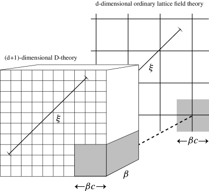
Figure 1: Dimensional reduction of a D-theory: Averaging the $(d+1)$-dimensional effective field of the D-theory over blocks of size $\beta$ in the extra dimension and $\beta c$ in the physical directions results in an effective $d$-dimensional Wilsonian lattice field theory with lattice spacing $\beta c$.

The continuum limit of the effective lattice theory is reached as $g=1/\beta\rho_{s}\rightarrow 0$, and hence as the extent $\beta$ of the extra dimension becomes large. Still, in physical units of $\xi$, the extent $\beta\ll\xi$ becomes negligible in this limit. In the continuum limit, the lattice spacing $\beta c$ of the effective 2-d Wilsonian lattice $O(3)$ model becomes large in units of the microscopic lattice spacing of the quantum spin system. Hence, D-theory introduces a discrete substructure underlying Wilson’s lattice theory. Due to exact blocking the lattice artifacts are entirely due to the microscopic D-theory lattice.

3 Continuous-Time Loop Cluster Simulation of the Heisenberg Model at Very Large Correlation Lengths$\,{}^{2}$

Soon after the discovery of high-temperature superconductivity in doped lamellar copper oxides it was found that the undoped compounds are 2-d spin-1/2 quantum antiferromagnets. Through experimental, theoretical, and numerical efforts much progress has been made in the understanding of these systems. In particular, detailed neutron scattering measurements [9] of the correlation length $\xi$ in the magnet $\mbox{Sr}_{2}\mbox{CuO}_{2}\mbox{Cl}_{2}$ were found to be in apparent good agreement with the $\mbox{CH}_{2}\mbox{N}_{2}$-formula eq.(5) — i.e. with 3-loop asymptotic scaling of the effective 2-d lattice $O(3)$ model resulting from dimensional reduction. However, neutron scattering measurements on higher-spin systems [9, 15] reveal a striking discrepancy with the $\mbox{CH}_{2}\mbox{N}_{2}$-formula. The puzzle concerning the applicability of 3-loop asymptotic scaling has recently been resolved by simulating the Heisenberg model at very large correlation lengths $\xi\approx 350,000a$ [16].

In the context of relativistic quantum field theory, where the lattice spacing serves as an ultraviolet cut-off that is ultimately removed, the question of asymptotic scaling is unphysical, because it involves the bare coupling constant. At low temperatures a 2-d quantum antiferromagnet induces a lattice action for an effective 2-d $O(3)$ model with lattice spacing $a^{\prime}=\beta c$, which is much larger than the microscopic lattice spacing $a$ of the quantum antiferromagnet, and which is determined by the physical temperature $T=1/\beta$. Hence, the question of asymptotic scaling becomes a physical issue. A priori, it is unclear for what values of $\xi$ one should expect asymptotic scaling for the effective 2-d lattice action. However, it is known that asymptotic scaling often sets in only at very large correlation lengths. For example, in the 2-d classical $O(3)$ model with the standard lattice action, 3-loop asymptotic scaling sets in at about $\xi\approx 10^{5}$ lattice spacings [17]. Hence, one might expect that the $\mbox{CH}_{2}\mbox{N}_{2}$-formula works only above $\xi\approx 10^{5}a^{\prime}=10^{5}\beta c$. However, the induced effective lattice action is not the standard action. Indeed, the effective action results from exact blocking of the chiral perturbation theory action of the magnons. This action receives cut-off effects only from the microscopic lattice with spacing $a$. In the limit $a\rightarrow 0$ the induced coarse lattice action would be a perfect action. This means that in D-theory the cut-off effects are due to the fine lattice spacing $a$, not due to the lattice spacing $a^{\prime}=\beta c$ of the induced $d$-dimensional effective Wilsonian theory. Based on this argument, one expects that in the quantum Heisenberg model 3-loop asymptotic scaling sets in at $\xi\approx 10^{5}a$. Indeed, this is observed in the numerical simulations.

How can one investigate correlation lengths in the range $\xi\approx 10^{5}a$? In the classical 2-d $O(3)$ model this was possible using finite-size scaling methods [18, 17]. To investigate the correlation length in the quantum Heisenberg model we use the same technique. The key observation of finite-size scaling is that the finite-volume correlation length $\xi(L)$ of a periodic system of spatial size $L\times L$ is a universal function of $\xi/L$, where $\xi$ is the correlation length of the infinite system. Inverting this relation one writes

$$\xi=Lf(1/z)=Lf(\xi(L)/L).$$ (7)

Here $z=L/\xi(L)$ is Fisher’s finite-size scaling variable, which is a renormalization group invariant measure of the physical volume. For the classical 2-d $O(3)$ model the universal function $f$ has already been determined very precisely [18, 17]. Since at low temperatures the quantum Heisenberg model reduces to a classical 2-d lattice $O(3)$ model, we can use the same universal function to deduce infinite volume results from finite-volume correlation length data. It is important that eq.(7) assumes universal behavior, i.e. scaling, but not asymptotic scaling. Hence, we can test the $\mbox{CH}_{2}\mbox{N}_{2}$-formula without bias.

The finite-size scaling function $f$ is very sensitive to small changes in the finite-volume correlation length $\xi(L)$. A small error in $\xi(L)$ generates large uncertainties in the infinite-volume correlation length $\xi$. Hence, one needs a very accurate numerical method to determine $\xi(L)$. Fortunately, for the quantum Heisenberg model a very efficient loop cluster algorithm exists [19, 7], which practically eliminates auto-correlations in the Monte Carlo data. Also, it is possible to construct improved estimators which drastically reduce statistical errors. The only remaining systematic error is due to the Suzuki-Trotter discretization of Euclidean time. Recently, it has been realized that the discretization of Euclidean time is not necessary for path integrals of discrete quantum systems [8]. This completely eliminates the systematic discretization error of previous methods. Also, it greatly reduces storage and computer time requirements, and thus allows us to work at very low temperatures.

We have performed simulations at inverse temperatures $J/T=0.5,1.0,...,3.5$ measuring the correlation length directly in a large volume $L\approx 6\xi$. For $J/T=4.0,4.5,...,12$ we have used the finite-size scaling technique. The continuous time loop cluster algorithm was used in a single cluster version, and an improved estimator has been implemented for the staggered correlation function. Correlation lengths are extracted using the second moment method [18, 17]. In all cases at least $10^{5}$ measurements have been performed. The numerical data for the infinite-volume correlation length $\xi$ are compared with experimental data and the $\mbox{CH}_{2}\mbox{N}_{2}$-result in fig.2.

Figure 2: The correlation length $\xi/a$: Experimental data (crosses) and numerical data (circles) are in apparent good agreement with the $\mbox{CH}_{2}\mbox{N}_{2}$-formula eq.(5) (dashed line).

The numerically accessible correlation lengths are more than three orders of magnitude larger than the experimental ones [9].

Focusing on small effects invisible in fig.2, fig.3 shows the deviation from 2-loop asymptotic scaling as a function of temperature.

Figure 3: Analysis of the correlation length $\xi$ as the asymptotic scaling regime is approached: $\xi$ is divided by the 2-loop result $\xi_{2}=(ec/16\pi\rho_{s})\exp(2\pi\rho_{s}/T)$, using the best-fit value $\rho_{s}=0.1800(5)$. The 3-loop result (dashed line) is accurate only for $\xi\approx 10^{5}a$, while the 4-loop regime (solid line) begins at $\xi\approx 10^{2}a$.

The correlation length data have been fitted simultaneously with previously obtained data for the staggered and uniform susceptibilities in cubic [7] and cylindrical [8] space-time geometries. Indeed, we find that asymptotic scaling at the 3-loop level of the $\mbox{CH}_{2}\mbox{N}_{2}$-formula sets in at correlation lengths of $\xi\approx 10^{5}a$, while a 4-loop fit works well already at $\xi\approx 10^{2}a$. When the massgap is included as a fit parameter, its fitted value agrees with the exact massgap at the 2 percent level. In the light of our numerical data, the apparent good agreement of the $\mbox{CH}_{2}\mbox{N}_{2}$-formula with the less accurate spin 1/2 experimental data at higher temperatures must be considered accidental. The large discrepancy between the $\mbox{CH}_{2}\mbox{N}_{2}$-formula and experimental data for higher-spin systems [9, 15] probably arises, because again 3-loop asymptotic scaling sets in only at very small temperatures, which are inaccessible to experiments. An investigation of the spin 1 case using the continuous-time loop cluster algorithm is presently in progress.

The computational effort for simulating the quantum Heisenberg model is compatible to using the Wolff cluster algorithm [20] directly in the 2-d $O(3)$ model. For gauge theories, on the other hand, no efficient cluster algorithm has been found in Wilson’s formulation of the problem. Recently, the first efficient cluster algorithm for a gauge theory with a continuous gauge group has been constructed for the $U(1)$ quantum link model [21]. If efficient cluster algorithms can be constructed also for non-Abelian quantum link models, numerical simulations of QCD will become more accurate than the ones using Wilson’s method.

4 QCD as a Quantum Link Model$\,{}^{3}$

In Wilson’s formulation of lattice gauge theory the parallel transporters $u_{x,\mu}$ are classical $SU(N)$ matrices defined on the links $(x,\mu)$ of a 4-d hypercubic lattice. The standard Wilson action takes the form

$$S[u]=-\sum_{x,\mu\neq\nu}\mbox{Tr}[u_{x,\mu}u_{x+\hat{\mu},\nu}u^{\dagger}_{x+\hat{\nu},\mu}u^{\dagger}_{x,\nu}].$$ (8)

By construction, this action is invariant under gauge transformations

$$u^{\prime}_{x,\mu}=\exp(i\vec{\alpha}_{x}\cdot\vec{\lambda})u_{x,\mu}\exp(-i\vec{\alpha}_{x+\hat{\mu}}\cdot\vec{\lambda}).$$ (9)

In D-theory the Wilson action is replaced by a quantum link model Hamilton operator

$$H=J\sum_{x,\mu\neq\nu}\mbox{Tr}[U_{x,\mu}U_{x+\hat{\mu},\nu}U^{\dagger}_{x+\hat{\nu},\mu}U^{\dagger}_{x,\nu}].$$ (10)

Wilson’s classical link matrices are turned into quantum link operators $U_{x,\mu}$. They still are $N\times N$ matrices, but now their elements are non-commuting operators acting in a finite Hilbert space. Of course, we want to maintain the gauge symmetry of the problem. In quantum link models, gauge invariance means that $H$ commutes with local generators $\vec{G}_{x}$ of gauge transformations at the site $x$, which obey the usual algebra

$$[G^{a}_{x},G^{b}_{y}]=2i\delta_{xy}f_{abc}G^{c}_{x}.$$ (11)

Under a unitary transformation $\prod_{x}\exp(i\vec{\alpha}_{x}\cdot\vec{G}_{x})$, representing a gauge transformation in Hilbert space, a quantum link variable transforms as

$$U^{\prime}_{x,\mu} = \prod_{y}\exp(-i\vec{\alpha}_{y}\cdot\vec{G}_{y})U_{x,\mu}\prod_{z}\exp(i\vec{\alpha}_{z}\cdot\vec{G}_{z})$$ (12)

$$= \exp(i\vec{\alpha}_{x}\cdot\vec{\lambda})U_{x,\mu}\exp(-i\vec{\alpha}_{x+\hat{\mu}}\cdot\vec{\lambda}).$$

This relation implies

$$[\vec{G}_{x},U_{y,\mu}]=\delta_{x,y+\hat{\mu}}U_{y,\mu}\vec{\lambda}-\delta_{x,y}\vec{\lambda}U_{y,\mu},$$ (13)

which can be satisfied when we introduce

$$\vec{G}_{x}=\sum_{\mu}(\vec{R}_{x-\hat{\mu},\mu}+\vec{L}_{x,\mu}).$$ (14)

Here $\vec{L}_{x,\mu}$ and $\vec{R}_{x,\mu}$ are generators of left and right gauge transformations of the link variable $U_{x,\mu}$. They are $2(N^{2}-1)$ generators of an $SU(N)_{L}\otimes SU(N)_{R}$ algebra on each link. The commutation relations of eq.(13) imply

$${[}\vec{L}_{x,\mu},U_{y,\nu}] = -\delta_{x,y}\delta_{\mu\nu}\vec{\lambda}U_{x,,\mu},$$

$${[}\vec{R}_{x,\mu},U_{y,\nu}] = \delta_{x,y}\delta_{\mu\nu}U_{x,\mu}\vec{\lambda}.$$ (15)

In D-theory, the real and imaginary parts of the elements of the link matrices are represented by $2N^{2}$ Hermitean operators. Together with the operators $\vec{L}_{x,\mu}$ and $\vec{R}_{x,\mu}$, these are $4N^{2}-2$ generators. The above commutation relations are those of an $SU(2N)$ algebra, which contains $SU(N)_{L}\otimes SU(N)_{R}$ as a sub-algebra. Of course, $SU(2N)$ has $4N^{2}-1$ generators, and indeed there is one more generator $T_{x,\mu}$, which obeys

$$[T_{x,\mu},U_{y,\nu}]=2\delta_{x,y}\delta_{\mu\nu}U_{x,\mu}.$$ (16)

Consequently,

$$G_{x}=\frac{1}{2}\sum_{\mu}(T_{x-\hat{\mu},\mu}-T_{x,\mu})$$ (17)

generates an additional $U(1)$ gauge transformation

$$U^{\prime}_{x,\mu} = \prod_{y}\exp(-i\alpha_{y}G_{y})U_{x,\mu}\prod_{z}\exp(i\alpha_{z}G_{z})$$ (18)

$$= \exp(i\alpha_{x})U_{x,\mu}\exp(-i\alpha_{x+\mu}).$$

Indeed, the Hamilton operator of eq.(10) is also invariant under the extra $U(1)$ gauge transformations and thus describes a $U(N)$ lattice gauge theory. The symmetry can be reduced to $SU(N)$ by adding the real part of the determinant of each link matrix to the Hamilton operator

$$H = J\sum_{x,\mu\neq\nu}\mbox{Tr}[U_{x,\mu}U_{x+\hat{\mu},\nu}U^{\dagger}_{x+\hat{\nu},\mu}U^{\dagger}_{x,\nu}]$$ (19)

$$+ J^{\prime}\sum_{x,\mu}\ [\mbox{det}U_{x,\mu}+\mbox{det}U^{\dagger}_{x,\mu}].$$

Due to the discrete nature of the quantum link variables, the above algebraic structure can be expressed entirely in terms of anticommuting operators

$$U^{ij}_{x,\mu} = c_{x,+\mu}^{i\dagger}c_{x+\hat{\mu},-\mu}^{j},$$

$$\vec{L}_{x,\mu} = \sum_{ij}c_{x,+\mu}^{i\dagger}\vec{\lambda}_{ij}c_{x,+\mu}^{j},$$

$$\vec{R}_{x,\mu} = \sum_{ij}c_{x+\hat{\mu},-\mu}^{i\dagger}\vec{\lambda}_{ij}c_{x+\hat{\mu},-\mu}^{j},$$

$$T_{x,\mu} = \sum_{i}(c_{x,+\mu}^{i\dagger}c_{x,+\mu}^{i}-c_{x+\hat{\mu},-\mu}^{i\dagger}c_{x+\hat{\mu},-\mu}^{i}).$$ (20)

Here $c_{x,\pm\mu}^{i\dagger}$ and $c_{x,\pm\mu}^{i}$ are creation and annihilation operators of colored fermions living on a link that emanates from the site $x$ in the $\pm\mu$-direction. In quantum link models these fermions can be viewed as constituents of the gluons, which we call rishons. The rishon operators obey canonical anticommutation relations

$$\{c^{i}_{x,\pm\mu},c^{j\dagger}_{y,\pm\nu}\} = \delta_{xy}\delta_{\pm\mu,\pm\nu}\delta_{ij},$$

$$\{c^{i}_{x,\pm\mu},c^{j}_{y,\pm\nu}\} = \{c^{i\dagger}_{x,\pm\mu},c^{j\dagger}_{y,\pm\nu}\}=0.$$ (21)

It is easy to show that the rishon number

$${\cal N}_{x,\mu}=\sum_{i}(c^{i\dagger}_{x+\hat{\mu},-\mu}c^{i}_{x+\hat{\mu},-\mu}+c^{i\dagger}_{x,+\mu}c^{i}_{x,+\mu}),$$ (22)

is conserved separately for each link. In rishon representation the determinant of a quantum link operator takes the form

$$\mbox{det}\ U_{x,\mu}=N!c^{1}_{x,+\mu}c^{1\dagger}_{x,-\mu}...c^{N}_{x,+\mu}c^{N\dagger}_{x,-\mu}.$$ (23)

The $U(N)$ symmetry can be reduced to $SU(N)$ via the determinant only when one works with exactly $N$ rishons on each link. This corresponds to working with the $(2N)!/(N!)^{2}$-dimensional representation of $SU(2N)$. Inserting the rishon representation of $U_{x,\mu}$ in the Hamilton operator, one can describe the quantum link dynamics as a hopping of rishons. This is illustrated in fig.4.

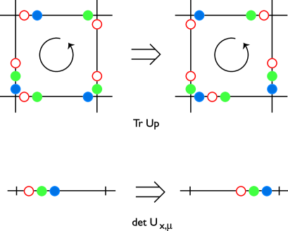
Figure 4: QCD dynamics as a rishon abacus: The trace part of the Hamiltonian induces hopping of rishons of various colors around a plaquette. The determinant part shifts a color-neutral combination of $N$ rishons from one end of a link to the other.

The partition function

$$Z=\mbox{Tr}\exp(-\beta H)$$ (24)

of a quantum link model defined on a 4-d lattice can be expressed as a $(4+1)$-d path integral. Note that we have not imposed the 5-d Gauss law, i.e., we have not included a projector on gauge invariant states propagating in the fifth direction. This implies that the fifth component of the non-Abelian vector potential, $A_{5}=0$, vanishes. This is important, because it leaves us with the correct field content after dimensional reduction. Note that the physical 4-d Gauss law is properly imposed, because the model does contain non-trivial Polyakov loops in the Euclidean time direction.

For quantum spin models, dimensional reduction arises naturally, because the spontaneous breakdown of a continuous global symmetry provides massless Goldstone modes, and hence an infinite correlation length. On the other hand, when a gauge symmetry breaks spontaneously, due to the Higgs mechanism there are no massless modes, and hence dimensional reduction would not occur. Also in a confined phase the correlation length is finite. However, non-Abelian gauge theories in five dimensions generically have a massless Coulomb phase [22]. Based on universality, it is natural to assume the presence of a massless Coulomb phase also for quantum link models. Then the 5-d massless Coulombic gluons are described by the low-energy effective action

$$S[A] = \int_{0}^{\beta}dx_{5}\int d^{4}x$$ (25)

$$\times \frac{1}{2e^{2}}[\mbox{Tr}\ F_{\mu\nu}F_{\mu\nu}+\frac{1}{c^{2}}\mbox{Tr}\ \partial_{5}A_{\mu}\partial_{5}A_{\mu}],$$

which is just the standard 5-d Yang-Mills action with $A_{5}=0$. The quantum link model is characterized by the “velocity of light” $c$, which is the analog of the spin-wave velocity in the Heisenberg model. Note that $\mu$ in eq.(25) runs over 4-d indices only. The dimensionful 5-d gauge coupling $1/e^{2}$ is the analog of $\rho_{s}$ in the spin model. At finite $\beta$ the above theory has a 4-d gauge invariance only, because $A_{5}=0$. At $\beta=\infty$ we are in the 5-d Coulomb phase with massless gluons, and hence with an infinite correlation length $\xi$. At finite $\beta$ the extent of the extra dimension becomes negligible compared to $\xi$, and the theory appears to be dimensionally reduced to four dimensions. However, in four dimensions the confinement hypothesis suggests that gluons are no longer massless. Then, as argued in refs.[1, 5], a finite correlation length

$$\xi\propto\exp(\frac{24\pi^{2}\beta}{11Ne^{2}})$$ (26)

is generated non-perturbatively. Here $24\pi^{2}/11N$ is the 1-loop $\beta$-function coefficient of $SU(N)$ gauge theory, and

$$1/g^{2}=\beta/e^{2}$$ (27)

is the gauge coupling of the dimensionally reduced 4-d theory. The continuum limit $g\rightarrow 0$ of the 4-d theory is reached when the extent $\beta$ of the fifth direction becomes large. Like the spin model, one can consider the dimensionally reduced 4-d theory as a Wilsonian lattice theory with lattice spacing $\beta c$ (which has nothing to do with the microscopic lattice spacing of the quantum link model). As before, one averages the 5-d field over cubic blocks of size $\beta$ in the fifth direction and of size $\beta c$ in the four physical space-time directions. The block centers form a 4-d space-time lattice of spacing $\beta c$, and the effective theory of the block averaged 5-d Coulombic gluons resembles a 4-d Wilsonian lattice gauge theory.

Higher dimensions play an important role also in string theory. For example, the five known superstring theories are anomaly free only in ten dimensions. The unifying low-energy effective theory of all these models is supergravity in eleven dimensions. The various string theories are just different 10-dimensional reductions of the same 11-dimensional effective theory. The coupling constant of the 10-d string theory is related to the 11-d supergravity coupling and to the extent of the extra dimension. Attempts to formulate string theory beyond perturbation theory have led to M-theory, which is a microscopic structure underlying the non-renormalizable 11-dimensional supergravity. A candidate for M-theory is a matrix model [23], in which the classical string coordinates $X_{\mu}$ are replaced by non-commuting operators. All this is remarkably similar to the D-theory formulation of QCD in four dimensions. First, the classical gluon field $A_{\mu}$ is replaced by non-commuting quantum link operators. The low-energy effective theory of the resulting D-theory is a non-renormalizable 5-d non-Abelian gauge theory. Finally, just as in string theory, the resulting gauge coupling of QCD in four dimensions $1/g^{2}=\beta/e^{2}$ is related to the 5-d gauge coupling $e$ and to the extent $\beta$ of the fifth direction. Due to these striking similarities, it seems that D-theory can be viewed as a daughter of M-theory — the string theorist’s candidate for the mother of all fundamental theories.

5 Numerical Verification of Dimensional Reduction in Wilsonian $SU(3)$ Lattice Gauge Theory$\,{}^{4}$

The above scenario of dimensional reduction crucially depends on the presence of a massless Coulomb phase in 5-d non-Abelian gauge theories. Early numerical evidence for a weak coupling phase in 5-d $SU(2)$ gauge theory was presented in ref.[22]. Here we extend these results to $SU(3)$ and establish that the weak coupling phase is indeed a massless Coulomb phase [24]. The corresponding numerical simulations are performed using Wilson’s formulation of lattice gauge theory. Via universality they should also apply to D-theory. Once cluster algorithms become available for non-Abelian quantum link models, the assumption of universality will be tested in detail.

First, 5-d pure $SU(3)$ lattice gauge theory has been simulated using the standard Wilson action on $4^{5}-8^{5}$ lattices. There is a strong first order phase transition separating the confined phase at strong coupling from a weak coupling phase. The phase transition is at $6/e_{0}^{2}=4.35(15)$. The question arises if the weak coupling phase is a massless Coulomb phase or a massive Higgs phase. To investigate this question, a Higgs model including an explicit scalar degree of freedom has been studied. In the unitary gauge, the action of the extended model is given by

$$S[U] = \frac{6}{e_{0}^{2}}\sum_{\Box}(1-\frac{1}{3}\mbox{Re Tr}U_{\Box})$$ (28)

$$+ \kappa\sum_{x,\mu}(1-\frac{1}{3}\mbox{Re Tr}U_{x,\mu}).$$

The phase diagram of the model is shown in fig.5.

Figure 5: The phase diagram of the 5-d $SU(3)$ Higgs model: The weak coupling Coulomb phase is separated from the Higgs-confinement phase by strong first order phase transitions.

The weak coupling phase of the pure gauge theory extends to small values of $\kappa$, but is separated from the Higgs phase at large $\kappa$ by a strong first order phase transition. The massive Higgs and confined phases are analytically connected.

To establish that the weak coupling phase of the pure gauge theory is indeed a massless Coulomb phase, the static quark potential has been investigated on a $16^{5}$ lattice at $6/e_{0}^{2}=4.6$ and 9.0 for $\kappa=0$. Wilson loops $W(R,T)$ of various sizes $(R,T)$ are measured and fitted to the functional form

$$W(R,T)=A\exp(-e^{2}F(R,T)),$$ (29)

where $F(R,T)$ is the lattice tree-level perturbative result. Fig.6 shows the fit for $6/e_{0}^{2}=4.6$.

Figure 6: Fit of Wilson loops: Loops of sizes $4\times 4$ to $8\times 8$ on a $16^{5}$ lattices at $6/e_{0}^{2}=4.6$ are fitted to a 5-d lattice Coulomb potential.

The fit parameters are $A=1.103(5)$, $e^{2}=2.525(2)$, and $\chi^{2}/\mbox{d.o.f.}=1.2(7)$. Similarly, for $6/e_{0}^{2}=9.0$ one obtains $A=1.0089(3)$, $e^{2}=0.8333(2)$, and $\chi^{2}/\mbox{d.o.f.}=0.8(2)$. As it should, the parameter $A$ approaches 1 in the $e_{0}\rightarrow 0$ limit. Also note that the charge renormalization $e^{2}/e_{0}^{2}$ drops from 1.936 at $6/e_{0}^{2}=4.6$ to 1.25 at $6/e_{0}^{2}=9.0$. Finally, when a massterm for the gauge bosons is included in the fit, its fitted value is consistent with zero. This confirms the presence of a massless weak coupling phase with a 5-d Coulomb potential $V(R)=e^{2}/R^{2}$.

To verify reduction from five to four dimensions, the 4-d finite temperature phase transition has been investigated using 5-d pure gauge theory with $A_{5}=0$. The extent $\beta$ in the fifth direction generates an effective 4-d gauge coupling $1/g^{2}=\beta/e^{2}$. The extent in the fourth (Euclidean time) direction is also finite, and corresponds to the inverse physical temperature. For practical purposes, it is necessary to work with asymmetric lattices with a coupling $6/e_{0}^{2}$ for the space-time plaquettes and a coupling $6/e_{5}^{2}$ for plaquettes involving the fifth direction. The simulations were done on $16^{3}\times 6\times 2$ lattices with $6/e_{0}^{2}=4.6$ and $6/e_{5}^{2}=2.41,...,2.49$. The Polyakov loop in the fourth (Euclidean time) direction is shown in fig.7.

Figure 7: Behavior of the 4-d Polyakov loop: Varying the coupling $6/e_{5}^{2}$ of plaquettes involving the fifth direction, a signal for a confinement-deconfinement phase transition is seen in the dimensionally reduced 4-d theory.

One sees a clear signal for a confinement-deconfinement phase transition in the dimensionally reduced 4-d theory. Of course, when one uses Wilson’s method, in the pure gauge theory there is no reason to go to five dimensions. Still, our results show that the expected dimensional reduction to ordinary 4-d physics actually takes place, when one chooses the coupling such that the 5-d system is in the Coulomb phase. If the quantum link model falls in the Coulomb phase, universality implies that it also undergoes dimensional reduction. Once cluster algorithms become available for non-Abelian quantum link models, this scenario will be tested in detail. If powerful cluster algorithms can be constructed, it is likely that working with a 5-d quantum link model is more efficient than using Wilson’s method in four dimensions.

6 Quantum Link QCD with Quarks$\,{}^{5}$

Let us now construct full QCD in the framework of D-theory. The construction principle of D-theory is to replace the classical action in Wilson’s formulation by a Hamilton operator. For fermions one also replaces $\bar{\psi}_{x}$ by $\Psi^{\dagger}_{x}\gamma_{5}$. Thus, the quantum link QCD Hamilton operator takes the form

$$H = J\sum_{x,\mu\neq\nu}\mbox{Tr}[U_{x,\mu}U_{x+\hat{\mu},\nu}U^{\dagger}_{x+\hat{\nu},\mu}U^{\dagger}_{x,\nu}]$$ (30)

$$+ J^{\prime}\sum_{x,\mu}\ [\mbox{det}U_{x,\mu}+\mbox{det}U^{\dagger}_{x,\mu}]$$

$$+ \frac{1}{2}\sum_{x,\mu}[\Psi^{\dagger}_{x}\gamma_{5}\gamma_{\mu}U_{x,\mu}\Psi_{x+\hat{\mu}}\!-\!\Psi^{\dagger}_{x+\hat{\mu}}\gamma_{5}\gamma_{\mu}U^{\dagger}_{x,\mu}\Psi_{x}]$$

$$+ M\sum_{x}\Psi^{\dagger}_{x}\gamma_{5}\Psi_{x}+\frac{r}{2}\sum_{x,\mu}\ [2\Psi^{\dagger}_{x}\gamma_{5}\Psi_{x}$$

$$- \Psi^{\dagger}_{x}\gamma_{5}U_{x,\mu}\Psi_{x+\hat{\mu}}-\Psi^{\dagger}_{x+\hat{\mu}}\gamma_{5}U^{\dagger}_{x,\mu}\Psi_{x}].$$

Here $\Psi^{\dagger}_{x}$ and $\Psi_{x}$ are quark creation and annihilation operators with canonical anticommutation relations

$$\{\Psi^{ia\alpha}_{x},\Psi^{jb\beta\dagger}_{y}\} = \delta_{xy}\delta_{ij}\delta_{ab}\delta_{\alpha\beta},$$

$$\{\Psi^{ia\alpha}_{x},\Psi^{jb\beta}_{y}\} = \{\Psi^{ia\alpha\dagger}_{x},\Psi^{jb\beta\dagger}_{y}\}=0,$$ (31)

where $(i,j)$, $(a,b)$ and $(\alpha,\beta)$ are color, flavor and Dirac indices, respectively. The generators of $SU(N)$ gauge transformation now take the form

$$\vec{G}_{x}=\sum_{\mu}(\vec{R}_{x-\hat{\mu},\mu}+\vec{L}_{x,\mu})+\Psi^{\dagger}_{x}\vec{\lambda}\Psi_{x}.$$ (32)

The dimensional reduction of fermions is not completely straightforward. When one uses antiperiodic boundary conditions in the extra dimension, the Matsubara modes, $p_{5}=2\pi(n_{5}+\frac{1}{2})/\beta$, lead to a short ${\cal O}(\beta)$ fermionic correlation length. Hence, from the point of view of the 4-d gluon dynamics, fermions with antiperiodic boundary conditions in the fifth direction stay at the cut-off and do not undergo dimensional reduction. When one uses periodic boundary conditions, a Matsubara mode, $p_{5}=0$, arises, and the quarks survive dimensional reduction, but we face the same fine-tuning problem that arises for Wilson fermions.

The fine-tuning problem has been solved very elegantly in Shamir’s variant [25] of Kaplan’s fermion proposal [26]. Kaplan coupled 5-d fermions to a 4-d domain wall, and found that a fermionic zero-mode gets bound to the wall. From the point of view of the dimensionally reduced theory, the zero-mode represents a 4-d chiral fermion. For QCD, Shamir has simplified Kaplan’s proposal by formulating the theory in a 5-d slab of finite size $\beta$ with open boundary conditions for the fermions at the two sides. This geometry fits naturally with the D-theory construction of quantum link models. With open boundary conditions for the quarks and with periodic boundary conditions for the gluons, the partition function takes the form

$$Z=\mbox{Tr}\langle 0|\exp(-\beta H)|0\rangle.$$ (33)

The trace extends over the gluonic Hilbert space only. Taking the expectation value in the Fock state $|0\rangle$, implies that there are no left-handed quarks at $x_{5}=0$, and no right-handed quarks at $x_{5}=\beta$ [27].

In the presence of quarks, the low-energy effective theory of the gluons (with $A_{5}=0$) must be modified to

$$S[\bar{\psi},\psi,A] = \int_{0}^{\beta}dx_{5}\int d^{4}x$$ (34)

$$\times \{\frac{1}{2e^{2}}[\mbox{Tr}F_{\mu\nu}F_{\mu\nu}+\frac{1}{c^{2}}\mbox{Tr}\partial_{5}A_{\mu}\partial_{5}A_{\mu}]$$

$$+ \bar{\psi}[\gamma_{\mu}(A_{\mu}+\partial_{\mu})\!+\!M\!+\!\frac{1}{c^{\prime}}\gamma_{5}\partial_{5}]\psi\}.$$

The “velocity of light” $c^{\prime}$ of the quarks in the fifth direction is expected to be different from the velocity $c$ of the gluons, because in D-theory there is no symmetry between the four physical space-time directions and the extra fifth direction. This is no problem, because we are only interested in the 4-d physics after dimensional reduction.

Due to confinement, after dimensional reduction the gluonic correlation length is exponentially large, but not infinite. As explained in ref.[5], the same is true for the quarks, but for a different reason. Even free quarks pick up an exponentially small mass due to tunneling between the two boundaries of the 5-d slab. The corresponding tunneling correlation length is $2M\exp(M\beta)$. This suggests how D-theory can avoid the fine-tuning problem that arises for Wilson fermions. In the chiral limit of quantum link QCD, the 4-d gluon dynamics takes place at a length scale

$$\xi\propto\exp(\frac{24\pi^{2}\beta}{(11N-2N_{f})e^{2}}),$$ (35)

which is determined by the 1-loop coefficient of the $\beta$-function of QCD with $N_{f}$ massless quarks and by the 5-d gauge coupling $e$. If one chooses

$$M>\frac{24\pi^{2}}{(11N-2N_{f})e^{2}},$$ (36)

the chiral limit is automatically approached before one reaches the continuum limit as $\beta$ becomes large. This solves the fermion doubling problem as well as the resulting fine-tuning problem in the D-theory formulation of QCD.

7 A Flux Cluster Algorithm for the $U(1)$ Quantum Link Model$\,{}^{6}$

Cluster algorithms have been extremely successful in solving lattice field theories with a global symmetry, like Ising and Potts models [28] as well as $O(N)$ models [20, 29] and $\Phi^{4}$ theory [30]. In these cases critical slowing down is practically eliminated, which allows very precise numerical simulations close to the continuum limit. In these cases, the clusters can be identified with physical excitations [31, 32]. The cluster size is related to a susceptibility, which implies that the clusters cannot grow beyond the physical correlation length. This is essential for the efficiency of these algorithms. For other models, like $CP(N)$ models with $N>1$ [33] and $SU(N)\otimes SU(N)$ chiral models with $N>2$, cluster algorithms can also be constructed. However, they turn out not to be efficient, as discussed in Ref.[34]. In these cases the clusters are not related to a physical quantity. For lattice gauge theories the situation is even more difficult. Only for models with discrete gauge groups efficient cluster algorithms could be found [35, 36]. Despite numerous attempts, so far no efficient cluster algorithm has been constructed for models with continuous gauge groups. These attempts failed due to the presence of frustrated interactions and difficulties to find an efficient embedding of discrete variables.

Here we construct the first efficient cluster algorithm for a model with a continuous gauge group — the $U(1)$ quantum link model. When formulated as a $(d+1)$-dimensional D-theory, this model is expected to reproduce the physics of the standard Wilson formulation of $d$-dimensional compact $U(1)$ gauge theory. For $d=4$ there is a phase transition between a strong coupling confined phase and a weak coupling massless Coulomb phase [37]. Due to the infinite correlation length of 5-d photons, dimensional reduction from 5 to 4 dimensions occurs when the extent $\beta$ of the additional fifth dimension becomes finite. As in non-Abelian quantum link models, one has $1/g^{2}=\beta/e^{2}$. Dimensional reduction occurs as long as the effective 4-d gauge coupling $g$ is weak enough to fall in the Coulomb phase of the 4-d theory. At stronger coupling, and hence at a smaller extent of the fifth direction, one enters the confined phase. Then the correlation length is finite, and dimensional reduction does not occur. For $d=3$ compact $U(1)$ gauge theory always confines [38, 39], but the correlation length diverges exponentially in the weak coupling limit. Then the mechanism of dimensional reduction is very similar to the one in QCD going from 5 to 4 dimensions. In particular, dimensional reduction occurs only when the extent of the extra dimension becomes large.

An efficient cluster algorithm for the $U(1)$ quantum link model can be constructed, because the variables are discrete even though the gauge symmetry is continuous. Hence, in contrast to Wilson’s formulation, no embedding problem arises. Also, the clusters are physical objects — namely world-sheets of electric flux strings propagating in the additional Euclidean dimension. The flux cluster algorithm is a gauge analog of the loop algorithm for the quantum Heisenberg model [19, 7]. Like the loop algorithm, it operates directly in the continuum of the additional Euclidean dimension [8]. Improved estimators for Wilson loops can also be constructed.

The Hamilton operator of the $U(1)$ quantum link model is defined on a $d$-dimensional lattice and is given by

$$H = -\frac{J}{2}\sum_{x,\mu<\nu}[U_{x,\mu}U_{x+\hat{\mu},\nu}U^{\dagger}_{x+\hat{\nu},\mu}U^{\dagger}_{x,\nu}$$ (37)

$$+ U_{x,\nu}U_{x+\hat{\nu},\mu}U^{\dagger}_{x+\hat{\mu},\nu}U^{\dagger}_{x,\mu}].$$

The quantum link operators $U_{x,\mu}$ and the generators of gauge transformations $G_{x}$ can be represented as

$$U_{x,\mu} = S_{x,\mu}^{1}+iS_{x,\mu}^{2}=S_{x,\mu}^{+},$$

$$G_{x} = \sum_{\mu}(S_{x-\hat{\mu},\mu}^{3}-S_{x,\mu}^{3}),$$ (38)

where $S^{i}_{x,\mu}$ is a spin operator associated with a link, with the usual commutation relations

$$[S_{x,\mu}^{i},S_{y,\nu}^{j}]=i\delta_{x,y}\delta_{\mu\nu}\varepsilon_{ijk}S_{x,\mu}^{k}.$$ (39)

The operator $S_{x,\mu}^{3}=T_{x,\mu}/2$ represents the electric flux, and $U_{x,\mu}$ acts as a flux raising operator.

The partition function

$$Z=\mbox{Tr}\exp(-\beta H)$$ (40)

can be formulated as a $(d+1)$-dimensional path integral. Here we describe the situation in $d=2$. Performing a checker board decomposition $H=H_{e}+H_{o}$ of the Hamiltonian into contributions of even and odd plaquettes, and discretizing the extra dimension into $N$ intervals of size $\varepsilon$, the partition function takes the form

$$Z=\lim_{\varepsilon\rightarrow 0}\mbox{Tr}\{[\exp(-\varepsilon H_{e})\exp(-\varepsilon H_{o})]^{N}\}.$$ (41)

Inserting complete sets of basis states between each pair of operators yields a $(2+1)$-dimensional lattice with $2N$ slices in the third dimension. Here we work in an electric flux basis, and we limit ourselves to spin 1/2, such that the eigenvalues of $S_{x,\mu}^{3}$ in the slice $n$ (with $n\in\{1,2,...,2N\}$) at $t=\varepsilon n/2$ are limited to $e_{x,\mu,t}=\pm 1/2$. The partition function then takes the form

$$Z=\prod_{x,\mu,t}\sum_{e_{x,\mu,t}=\pm 1/2}\exp(-S[e]).$$ (42)

The action $S[e]$ is a sum of contributions from checker boarded cubes carrying an 8-link interaction. The Boltzmann factor of a cube is determined by the elements of the $16\times 16$ plaquette transfer matrix

$${\cal T} = \exp(\varepsilon\frac{J}{2}[U_{x,\mu}U_{x+\hat{\mu},\nu}U^{\dagger}_{x+\hat{\nu},\mu}U^{\dagger}_{x,\nu}$$ (43)

$$+ U_{x,\nu}U_{x+\hat{\nu},\mu}U^{\dagger}_{x+\hat{\mu},\nu}U^{\dagger}_{x,\mu}]).$$

All diagonal elements of the transfer matrix are 1, except $\langle++--|{\cal T}|++--\rangle=\langle--++|{\cal T}|--++\rangle=\cosh(\varepsilon J/2)=c$, and all off-diagonal elements vanish, except $\langle++--|{\cal T}|--++\rangle=\langle--++|{\cal T}|++--\rangle=\sinh(\varepsilon J/2)=s$. Here, $\pm$ denotes the electric fluxes $e_{x,\mu}$, $e_{x+\hat{\mu},\nu}$, $e_{x+\hat{\nu},\mu}$, $e_{x,\nu}$ around a plaquette in two adjacent time-slices.

The cluster algorithm constructs open or closed oriented surfaces, which represent world-sheets of electric flux strings propagating in the extra dimension. An update reverses the flux of all links belonging to the cluster. Cluster growth starts by selecting an initial link $(x,\mu,t)$ at random. The flux variable $e_{x,\mu,t}$ participates in two cube interactions, one at earlier, the other at later $t$ values. The eight links of a cube are connected to clusters according to the following rules. For a cube configuration of weight $c$, with a probability $p=(c-s+7)/8c$ each link is connected to its $t$-partner shifted in the extra dimension. With probability $1-p$ the links are connected in two groups of four links, such that the four links with the same $t$ value are connected. For a configuration of weight 1, with a probability $q=(c-s+7)/8$ each link is connected to its $t$-partner. With probability $1-q$ the links are connected in two groups of four, such that after flipping one group, a configuration of weight $s$ is obtained. For a configuration of weight $s$, with probability $r=(7c+s-7)/8s$ the four links with the same $t$-value are connected. With probability $(1-r)/7$ they are connected in two groups of four, such that after flipping one group, one of the fourteen weight 1 configurations is obtained. The generated clusters form open or closed surfaces. The open surfaces arise, because we have not imposed the 5-d Gauss law for states propagating in the extra dimension. The algorithm is constructed such that it obeys ergodicity and detailed balance.

Due to the discrete basis of the Hilbert space, the path integral expression for the partition function of eq.(41) is well-defined in the continuum of the extra dimension, i.e., at $\varepsilon=0$. Taking the continuum limit of the cluster rules, one obtains an algorithm that operates directly in the continuum of the extra dimension. This algorithm has been implemented along the lines of the continuous-time loop-cluster algorithm for the quantum Heisenberg model [8].

To show that the clusters are directly related to physical objects, we consider the expectation values of Wilson loops $W_{\cal C}$ — the product of quantum link operators $U_{x,\mu}$ along some closed curve ${\cal C}$ on the $d$-dimensional lattice at a fixed value of $t$. The quantum links act as raising operators of electric flux. Hence, a configuration contributing to $\langle W_{\cal C}\rangle$ is inconsistent with the constraints in the configurations contributing to $Z$. Thus, it seems that just using the flux cluster algorithm does not provide information about Wilson loops. However, one can imagine flipping only a part of a cluster, which is bounded by a curve ${\cal C}$. This leads into the right sector for collecting information about $\langle W_{\cal C}\rangle$. In practice, one need not even perform these partial cluster flips explicitly, because one can extract the same information by examining the clusters of the original algorithm. This leads to an improved estimator for Wilson loops, which only receives positive contributions from each cluster, and shows that the clusters themselves represent physical objects. To verify the efficiency of the algorithm we have measured autocorrelation times, which indeed are small. A detailed study of the dynamical critical exponent $z$ is in progress.

The flux cluster algorithm operating in the continuum of the extra dimension has been applied to the $(4+1)$-dimensional and $(3+1)$-dimensional $U(1)$ quantum link models. In the $(4+1)$-dimensional model the cluster size per 5-d volume $|C|/V$ is shown as a function of the extent $\beta$ of the fifth direction in fig.8.

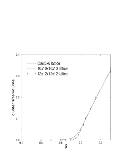
Figure 8: Cluster area per 5-d volume in the $(4+1)$-d $U(1)$ quantum link model: Above the critical extent $\beta_{c}\approx 0.65$ of the fifth direction, the cluster size increases with the volume, indicating the presence of a Coulomb phase with an infinite correlation length.

Above $\beta_{c}\approx 0.65$ the cluster size is proportional to the volume, indicating the infinite correlation length in the Coulomb phase. As shown in fig.9, in the $(3+1)$-dimensional model, $|C|/V$ goes to zero when one increases the volume, which is consistent with a confined phase for all $\beta$.

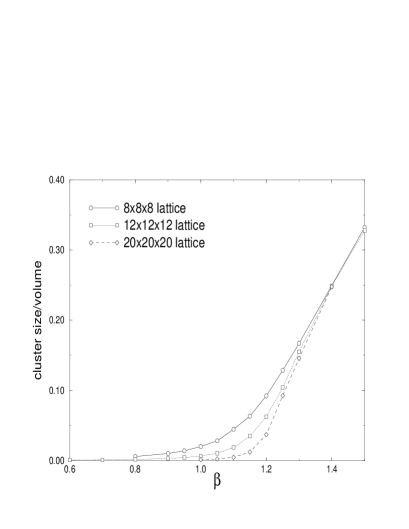
Figure 9: Cluster area per 4-d volume in the $(3+1)$-d $U(1)$ quantum link model: The data are consistent with a confined phase for all extents $\beta$ of the fourth direction.

As expected, a large increase of the cluster size is observed in the large $\beta$ limit. A detailed investigation of Wilson loops in $d=3$ and $d=4$ using improved estimators is in progress.

8 Conclusions

D-theory provides a new non-perturbative formulation of quantum field theory. Dimensional reduction of discrete variables is a generic phenomenon that occurs for various models, including $O(N)$, $CP(N)$, and $SU(N)\otimes SU(N)$ scalar models, as well as Abelian and non-Abelian gauge theories, in particular QCD. The discrete nature of the fundamental variables makes D-theory attractive, both from an analytic and from a computational point of view. On the analytic side, the discrete variables allow us to rewrite the bosonic fields in terms of fermionic rishon constituents. This may turn out to be useful for studying the large $N$ limit. On the numerical side powerful cluster algorithms become available, which may dramatically improve numerical simulations of lattice field theories. A lot of work needs to be done to decide if D-theory provides a more efficient non-perturbative quantization of field theories than Wilson’s method.

References

- [1] S. Chandrasekharan and U.-J. Wiese, Nucl. Phys. B492 (1997) 455.
- [2] D. Horn, Phys. Lett. 100B (1981) 149.
- [3] P. Orland and D. Rohrlich, Nucl. Phys. B338 (1990) 647.
- [4] R. Brower, S. Chandrasekharan and U.-J. Wiese, in preparation.
- [5] R. Brower, S. Chandrasekharan and U.-J. Wiese, hep-th/9704106.
- [6] T. Barnes, Int. J. Mod. Phys. C2 (1991) 659.
- [7] U.-J. Wiese and H.-P. Ying, Z. Phys. B93 (1994) 147.
- [8] B. B. Beard and U.-J. Wiese, Phys. Rev. Lett. 77 (1996) 5130.
- [9] M. Greven et al., Phys. Rev. Lett. 72 (1994) 1096; Z. Phys. B96 (1995) 465.
- [10] P. Hasenfratz and H. Leutwyler, Nucl. Phys. B343 (1990) 241.
-
[11]
N. D. Mermin and H. Wagner, Phys. Rev. Lett. 17 (1966) 1133;
S. Coleman, Commun. Math. Phys. 31 (1973) 259. - [12] S. Chakravarty, B. I. Halperin and D. R. Nelson, Phys. Rev. B39 (1989) 2344.
- [13] P. Hasenfratz and F. Niedermayer, Phys. Lett. B268 (1991) 231.
-
[14]
P. Hasenfratz, M, Maggiore and F. Niedermayer, Phys. Lett. B245 (1990) 522;
P. Hasenfratz and F. Niedermayer, Phys. Lett. B245 (1990) 529. - [15] K. Nakajima et al., Z. Phys. B96 (1995) 479.
- [16] B. B. Beard, R. J. Birgeneau, M. Greven and U.-J. Wiese, cond-mat/9709110.
- [17] S. Caracciolo et al., Phys. Rev. Lett. 75 (1995) 1891.
- [18] J. K. Kim, Phys. Rev. Lett. 70 (1993) 1735; Phys. Rev. D50 (1994) 4663.
- [19] H. G. Evertz, G. Lana and M. Marcu, Phys. Rev. Lett. 70 (1993)
- [20] U. Wolff, Phys. Rev. Lett. 62 (1989) 361; Nucl. Phys. B334 (1990) 581.
- [21] M. Basler, B. B. Beard, R. Brower, S. Chandrasekharan, A. Tsapalis and U.-J. Wiese, in preparation.
- [22] M. Creutz, Phys. Rev. Lett. 43 (1979) 553.
- [23] T. Banks, W. Fischler, S. H. Shenker and L. Susskind, Phys. Rev. D55 (1997) 5112.
- [24] R. Brower, S. Chandrasekharan, D. Chen and U.-J. Wiese, in preparation.
- [25] Y. Shamir, Nucl. Phys. B406 (1993) 90.
- [26] D. B. Kaplan, Phys. Lett. B288 (1992) 342.
- [27] V. Furman and Y. Shamir, Nucl. Phys. 439 (1995) 54.
- [28] R. Swendsen and S.-J. Wang, Phys. Rev. Lett. 58 (1987) 86.
- [29] P. Tamayo, R.C. Brower and W. Klein, J. Stat. Phys. 58 (1990) 1083.
- [30] R.C. Brower and P. Tamayo, Phys. Rev. Lett. 62 (1989) 1087.
- [31] C.M. Fortuin and P.W. Kasteleyn, Physica 57 (1972) 536.
- [32] A. Coniglio and W. Klein, J. Phys. A13 (1980) 2775.
- [33] K. Jansen and U.-J. Wiese, Nucl. Phys. B370 (1992) 762.
- [34] S. Caracciolo, R.G. Edwards, A. Pelisetto and A.D. Sokal, Nucl. Phys. B403 (1993) 475.
- [35] R. Ben-Av et al., J. Stat. Phys. 58 (1990) 125.
- [36] R.C. Brower and S. Huang, Phys. Rev. D41 (1990) 708; D44 (1991) 3911.
- [37] A. Guth, Phys. Rev. D21 (1980) 2291.
- [38] A.M. Polyakov, Phys. Lett. B59 (1975) 82.
- [39] M. Göpfert and G. Mack, Commun. Math. Phys. 82 (1982) 545.