HIP–1997–53/TH
September 12, 1997
Comparing improved actions for SU(2)

Abstract

In order to help the user in choosing the right action a performance comparison is done for seven improved actions. Six of them are Symanzik improved, one at tree-level and two at one-loop, all with or without tadpole improvement. The seventh is an approximate fixed point action. Observables are static on- and off-axis two-body potentials and four-body binding energies, whose precision is compared when the same amount of computer time is used by the programs.

We were motivated to consider using improved actions after noting the slowness of a four-quark flux distribution measurement code. In this case the lattice spacing has to be small, $a\approx 0.1$ fm, to achieve sufficient resolution. In this work we compare actions at that scale and at $a\approx 0.2$ fm.

1 The actions

The perturbative Symanzik approach to improvement is in this work represented by three actions; a tree-level version with a plaquette and a $1\times 2$ rectangle [1] (abbreviation: S) and two one-loop actions, one with a $1^{3}$ parallelogram (x,y,z,-x,-y,-z) [1, 2] (S1) and the other with both parallelogram and a $2\times 2$ large square [3] (S1S) as additional operators. Of these also the tadpole improved (TI) versions (STI, S1TI, S1STI) are considered. TI for the S1 action follows Ref. [4] using results for SU(2) in Ref. [2].

The non-perturbative approach to improvement is represented by a truncated fixed point action (FP) which includes first to fourth powers of the plaquette and the parallelogram [5].

2 The task

The measurements consist of static two-quark potentials for $R=1,\ldots,6$ on-axis, $R=(1,1),(2,1),\ldots,(3,3)$ off-axis and the binding energies of four quarks at the corners of a regular tetrahedron, the cube surrounding it having sides of length $R=1,2,3$. Here binding energies mean $E_{4}-2V_{2}$, where $E_{4}$ is the energy of four quarks and $2V_{2}$ the energy of the lowest-lying two-body pairing – see [6, 7].

In order to separate the ground state a variational basis of fuzzing levels 13 and 2 is used. An update step consisted of four overrelaxations and one heatbath sweep, except for the FP case for which the latter was replaced by ten Metropolis sweeps. Table 1 shows the $\beta$ values and corresponding scales used for the comparison. Scales were set by fitting plateau two-body potentials at $R=2,\ldots,6$ with the continuum parameterization $V_{\rm fit}=-e/R+b_{S}R+V_{0}$ and using Sommer’s equation $r_{0}^{2}F(r_{0})=c$ with $c=2.44$, corresponding to $r_{0}\approx 0.66$ fm. These scales agree with the determination using $\sqrt{b_{S}}=440$ MeV. The plateau was taken to be reached when the difference of potentials at $T+1$ and $T$ was smaller than the bootstrap error on this difference.

	$a\approx 0.1$ fm		$a\approx 0.2$ fm
Action	$\beta$	$a$ [fm]	$\beta$	$a$ [fm]
W	2.45	0.101(3)	2.23	0.204(3)
S	1.86	0.092(5)	1.63	0.197(5)
STI	1.98	0.097(2)	1.73	0.202(4)
S1	3.45	0.096(4)	3.03	0.198(2)
S1TI	3.5	0.097(3)	3.065	0.211(7)
S1S	3.65	0.097(5)	3.23	0.202(3)
S1STI	3.75	0.094(4)	3.33	0.196(4)
FP	1.69	0.101(3)	1.502	0.213(5)

Table 1:

The runs at $a\approx 0.1$ fm ($a\approx 0.2$ fm) on a $16^{4}$ ($12^{4}$) lattice consisted of 1000 (2500) measurements and were performed on SGI R10000 workstations. In the following, unless noted otherwise, we take a subset of these corresponding to the same amount of total CPU time consumed.

3 Results

CPU time: Table 2 shows the CPU time per update and per update+measurement relative to the Wilson action (W) – the measurements should take the same amount of time. Variations in consumption for two different actions using the same operators (one of them TI) reflect mostly the systematic errors in our time measurement. These are probably due to variations of CPU load and free memory.

The autocorrelation times of the plaquette average do not seem to depend on the size of the operators in the action.

	$a\approx 0.1$ fm		$a\approx 0.2$ fm
	upd./tot.	a.c.	upd./tot.	a.c.
W	1/1	1.9(4)	1/1	3.5(6)
S	3.3/1.2	2.1(5)	3.6/1.4	4.5(9)
STI	2.9/1.1	1.3(2)	3.5/1.4	3.3(6)
S1	7.9/1.5	1.6(4)	9.3/2.2	2.5(4)
S1TI	8.0/1.5	1.9(5)	9.6/2.3	2.4(4)
S1S	11.2/1.8	2.3(8)	12.0/2.7	2.7(5)
S1STI	12.4/1.8	1.7(4)	10.4/2.4	4.5(9)
FP	12.4/1.8	0.5(5)	10.4/2.4	3.0(5)

Table 2: CPU time and autocorrelation.

Plateaux: Actions which violate reflection positivity with negative eigenvalues of the Hamiltonian usually have a local maximum in the $M_{\rm eff}$ plot before a plateau is reached. When comparing the behaviour with the same number of measurements used, TI improves the plateau after this ’bump’, most notably for the STI case at $a\approx 0.1$ fm, which means that less correlators are needed. This can be used to save CPU time. Wilson and FP actions also have good plateaux and do not violate reflection positivity.

Statistical errors and rotational variance: Table 3 shows the average relative errors, which are statistical for all other observables except for the off-axis two-body potentials (Fig. 1), for which the deviation $|V_{\rm meas}-V_{\rm fit}|/V_{\rm fit}$ from the value given by the on-axis fit is also shown. The best improved actions are seen to have less rotational variance at $a\approx 0.2$ fm than the Wilson action at $a\approx 0.1$ fm.

	$a\approx 0.1$ fm			$a\approx 0.2$ fm
	on-	off-axis	4q	on-	off-axis
W	0.37	1.39(9)	4.8	0.29	2.35(9)
S	0.54	0.72(16)	4.4	0.66	1.23(13)
STI	0.36	0.58(9)	2.2	0.41	0.93(18)
S1	0.56	0.66(14)	5.3	0.59	0.97(12)
S1TI	0.49	0.68(11)	4.9	0.37	0.46(17)
S1S	0.86	0.83(22)	6.3	0.5	1.72(20)
S1STI	0.90	0.67(23)	3.1	0.9	0.83(16)
FP	0.43	0.49(10)	3.1	0.54	1.77(46)

Table 3: Average errors ($\times 100$) in two-body potentials and four-body binding energies.

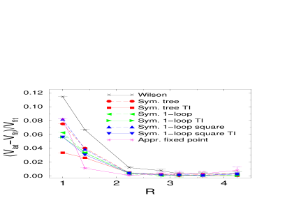
Figure 1: Rotational variance and statistical error for off-axis potentials at $a\approx 0.1$ fm.

Scaling: Figs. 2 and 3 show the differences of measured potentials from a fit to Wilson action data at $\beta=2.85$ [8], corresponding to $a\approx 0.027$ fm. In table 4 the averages of these differences are shown. None of the improved actions at $a\approx 0.2$ fm can be seen to scale as well as the Wilson action at $a\approx 0.1$ fm.

	$a\approx 0.1$ fm	$a\approx 0.2$ fm
W	0.020(4)	0.052(7)
S	0.015(7)	0.063(12)
STI	0.012(4)	0.042(11)
S1	0.022(7)	0.045(10)
S1TI	0.009(6)	0.039(11)
S1S	0.027(11)	0.047(11)
S1STI	0.013(10)	0.043(15)
FP	0.027(6)	0.064(13)

Table 4:

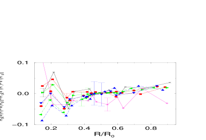
Figure 2: Difference of $a\approx 0.1$ fm potentials from those at $a=0.027$ fm. For each action one error bar is shown.

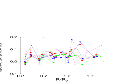
Figure 3: As Fig. 2 but for $a\approx 0.2$ fm

Self-energies: The lattice self-energies of the quarks given by the on-axis fit vary up to 40 % between different actions. In lowest-order perturbation theory this is due to the different lattice one-gluon exchange operators.

4 Discussion

For two-body potentials rotational invariance is improved significantly, while statistical errors are not – with the same amount of computer time used the Wilson action has the smallest statistical errors. The improvement in scaling seems to be small. For Symanzik improved actions TI works; statistical errors, rotational variance and scaling violations are reduced. Our only representative of truncated FP actions performs well at $a\approx 0.1$ fm, but has problems at the coarser $a$.

When using an improved action further improvement can be achieved with improved operators, which can also be essential for correct physics e.g. in lattice sum rules. Technical difficulties associated with improved operators include the separation of field components, for which planar actions (in this work S, STI) are easier. Other means of improvement include anisotropic lattices, lookup tables for loop collection, cache optimization and tuning the fuzzing parameters. Some of the latter three can be quite easily implemented with possibly a significant time-saving effect.

Acknowledgement: We thank A.M. Green and C. Michael for support and discussions, the Finnish Academy (P.P) and Magnus Ehrnrooth Foundation for funding and the Helsinki Institute of Physics for hospitality and computing facilities.

References

- [1] M. Luscher and P. Weisz, Commun. Math. Phys. 97, 59 (1985) and Phys. Lett. 158B, 250 (1985).
- [2] P. Weisz and R. Wohlert, Nucl. Phys. B236, 397 (1984).
- [3] J. Snippe, Phys. Lett. B389, 119 (1996).
- [4] M. Alford et al., Phys. Lett. B361, 87 (1995).
- [5] T. DeGrand, A. Hasenfratz and D. cai Zhu, Nucl. Phys. B478, 349 (1996).
- [6] A. M. Green, J. Lukkarinen, P. Pennanen and C. Michael, Phys. Rev. D 53, 261 (1996).
- [7] P. Pennanen, Phys. Rev. D 55, 3958 (1996).
- [8] S. P. Booth et al., Nucl. Phys. B394, 509 (1993).