BUTP-97/24

The fixed point action for the Schwinger model:
a perturbative approach

Federico Farchioni and Victor Laliena

Institute for Theoretical Physics

University of Bern

Sidlerstrasse 5, CH-3012 Bern, Switzerland

March 2024

Abstract

We compute the fixed point action of a properly defined renormalization group transformation for the Schwinger model through an expansion in the gauge field. It is local, with couplings exponentially suppressed with the distance. We check its perfection by computing the 1-loop mass gap at finite spatial volume, finding only exponentially vanishing cut off effects, in contrast with the standard action, which is affected by large power-like cut off effects. We point out that the 1-loop mass gap calculation provides a check of the classical perfection of the fixed point action, and not of the 1-loop perfection, as could be naively expected.

1 Introduction.

The discretization of the space-time into a lattice provides a non-perturbative regularization of a quantum field theory which, in addition, allows numerical simulations. The lattice spacing is finite in any Monte Carlo simulation, and the distortions on the physical quantities induced by the discretization (cut off effects) strongly restrict the accuracy of the method. The naive procedure - consisting in approaching the continuum by progressively reducing the lattice spacing - has to cope soon with the problem of the divergence of computational time and memory space. Therefore, new methods have been studied in order to reduce the lattice artifacts at their origin, i.e. at the level of the lattice action.

The first method, due to Symanzik, consists in adding to the simplest discretized action (standard action) higher order operators which cancel the cut off effects to a given order in the lattice spacing (usually the leading one, $O(a^{2})$ for bosonic theories and $O(a)$ in presence of fermions) and in the coupling constant; this method is designed for perturbation theory.

The second method uses the Wilson Renormalization Group (RG) theory, and is inherently non-perturbative. In this case, one can be very ambitious and search for perfect actions [1], which, by definition, reproduce exactly the continuum independently of the value of the lattice spacing. The existence of perfect actions follows from the existence of a renormalized trajectory in the space of parameters of the theory: any action located on the renormalized trajectory is a perfect action [1].

A more modest and realistic goal is the determination of a classically perfect action, i.e. an action which - in principle - eliminates the cut off effects with restriction to the classical properties of the theory. This action is related [1] to the fixed point (FP) - lying on the critical surface - of a given RG transformation. In the case of a theory which attains the continuum for weak couplings, the FP problem is reduced to the solution of a saddle point equation. Although not perfect, the FP action represents a huge step toward the elimination of the cut off effects in comparison with naive discretizations, and a considerable improvement is observed even with respect to the Symanzik improved actions [1, 2, 3].

In view of an application of these ideas to the numerical solution of lattice QCD, the fermion sector must be well understood. FP actions for gauge theories with interacting fermions have not been extensively studied yet. In this paper we will study the fermion-gauge field FP interactions in a much simpler case than QCD, the Schwinger model, which belongs to the class of theories for which the computation of a FP action is a classical saddle point problem. Since its gauge group is abelian, it is possible to formulate the lattice regularization with non-compact gauge fields, and to solve analytically the pure gauge sector. Therefore, we are able to concentrate the numerical effort in the fermion problem. We will test the perfection of the FP action by computing the 1-loop mass gap in a finite volume - a circle of length $L$ - using the standard action as a “control” action.

The remaining of the paper is organized as follows. In Section 2 we review briefly the formalism of the FP actions. In Section 3 we recall some features of the Schwinger model which are relevant for this work. Section 4 is devoted to the study of the FP action for the pure gauge sector. In Section 5 we address ourselves to the computation of the fermion part of the FP action; the problem is treated perturbatively - i.e. in an expansion in the gauge field. In Section 6 we check the perfection of the FP action, providing the computation of the mass gap to 1-loop. For comparison, we compute the mass gap also for the standard action. We end the paper with a discussion about the 1-loop perfection of the FP action (Section 7) and the conclusions (Section 8).

2 Fixed point actions.

In this Section we briefly describe the general method for the computation of the FP action in the case of theories reaching the continuum for small couplings, referring to the literature [4, 5, 6] for the details. For the sake of definiteness, we restrict the notation to case of the $U(1)$ gauge group in the non-compact formulation.

A general form of the action of a lattice-regularized gauge theory is

$$S\;=\;\beta\,S_{g}(A)\>+\>\bar{\psi}\,\Delta(U)\,\psi\,,$$ (1)

where $A$ denotes the gauge field configuration; $\Delta$ is a suitable fermion matrix which depends on the gauge field through the link variable $U_{\mu}=\exp(iA_{\mu})$. The detailed form of the action is here not relevant, apart from the requirement of gauge invariance and recovering of the classical continuum limit. In the fermion sector some care is necessary in order to ensure that the doublers decouple in the continuum limit. The partition function is given by the path integral

$${\cal Z}\;=\;\int\,\left[dA\,d\bar{\psi}\,d\psi\right]\,\exp\,\left[\,-\,\beta\,S_{g}(A)\>-\>\bar{\psi}\,\Delta(U)\,\psi\,\right]\,.$$ (2)

A RG transformation can be defined, which maps the action $S$ onto $S^{\prime}$, the latter action depending on fields defined on a coarser lattice:

$$\exp\,\left[\,-\,\beta^{\prime}\,S_{g}^{\prime}(A^{\prime})\>-\>S_{F}^{\prime}(\bar{\psi}^{\prime},\psi^{\prime},U^{\prime})\,\right]\;=$$

$$\hskip 28.45274pt\int\,\left[dA\,d\bar{\psi}\,d\psi\right]\,\exp\,\left[-\,\beta\,S_{g}(A)\>-\>\bar{\psi}\,\Delta(U)\,\psi\>-\>p\,{\cal K}_{g}(A^{\prime},A)\right.$$

$$\hskip 28.45274pt\left.-\>\kappa_{F}\,{\cal K}_{F}(\bar{\psi}^{\prime},\psi^{\prime},\bar{\psi},\psi,U)\,\right]\,,$$ (3)

where the primed fields are the degrees of freedom on the coarser lattice, defined through the gauge invariant kernels  ${\cal K}_{g}$  and  ${\cal K}_{F}$. The parameters $p$ and $\kappa_{F}$ can be chosen arbitrarily; in particular, we can take $p=\beta\,\kappa_{g}$. Note that in general the fermion action is not quadratic in the fermion fields after a RG transformation.

In the class of theories under interest (including asymptotically free non-abelian gauge theories and the Schwinger model), the critical surface (where the continuum is attained) is at $\beta=\infty$. The iteration of the RG transformation starting on this surface converges to a FP. When $\beta\rightarrow\infty$ the integral on the gauge degrees of freedom in the r.h.s. of Eq. (3) is saturated by the saddle point configuration; the solution of the recursion is then:

$$S_{g}^{\prime}(A^{\prime})\;=\;\min_{\{A\}}\,\left[S_{g}(A)\>+\>\kappa_{g}\,{\cal K}_{g}(A^{\prime},A)\,\right]\,,$$ (4)

$$S_{F}^{\prime}(\bar{\psi}^{\prime},\psi^{\prime},U^{\prime})\;=\;-\ln\,\int\,\left[d\bar{\psi}\,d\psi\right]\,\exp\,\left[\,-\>\bar{\psi}\,\Delta(U(A^{\textstyle\scriptscriptstyle min}))\,\psi\right.$$

$$\left.\;\;\;\;\;\;\;\;\;\;\;\;\;\;\;\;\;\;\;\;\;\;\;\;\;\;\;\;\;\;\;\;\;\;\;\;-\>\kappa_{F}\,{\cal K}_{F}(\bar{\psi}^{\prime},\psi^{\prime},\bar{\psi},\psi,U(A^{\textstyle\scriptscriptstyle min}))\,\right]\,,$$ (5)

where $A^{\textstyle\scriptscriptstyle min}$ is the fine gauge field configuration which minimizes the r.h.s. of Eq. (4), depending on the coarse configuration $A^{\prime}$; of course: $\beta^{\prime}=\beta=\infty$. In this limit the problem is equivalent to a classical minimization problem plus a Grassmann integration.

If the fermion kernel is quadratic in the fermion fields, the fermion action at $\beta=\infty$ remains quadratic after a RG transformation, as is evident from Eq. (5). The FP action is defined as:

$$S^{\scriptscriptstyle FP}\;=\;\beta\,S^{\scriptscriptstyle FP}_{g}(A)\>+\>\bar{\psi}\,\Delta^{\scriptscriptstyle FP}(U)\,\psi\,,$$ (6)

where $S^{\scriptscriptstyle FP}_{g}$ and $\Delta^{\scriptscriptstyle FP}$ are the self-reproducing solutions of Eq. (4) and Eq. (5) respectively. The FP action is then bilinear in the fermion fields; this is a very important issue, mainly for what concerns numerical simulations.

3 General considerations about the Schwinger model.

3.1 The continuum Schwinger model.

In this Section we shall review some features of the Schwinger model which are relevant for the following. The Schwinger model is the transcription to $1+1$ dimensions of the usual $3+1$ QED [7]. Its euclidean lagrangian reads (for the massive model):

$${\cal L}\;=\;\frac{1}{4}\,\sum_{\mu\nu}F_{\mu\nu}(x)F_{\mu\nu}(x)\>+\>\bar{\psi}(x)\,\left[\,\sum_{\mu}\gamma_{\mu}\partial_{\mu}\>+\>i\,e\,\sum_{\mu}\gamma_{\mu}\,A_{\mu}(x)\>+\>m_{f}\,\right]\,\psi(x)\,.$$ (7)

We use the simplest representation of the euclidean Dirac matrices in $1+1$ dimensions, given by the Pauli matrices:

$$\gamma_{0}\;=\;\sigma_{1}\,,\;\;\;\;\;\;\;\;\gamma_{1}\;=\;\sigma_{2}\,,\;\;\;\;\;\;\;\;\gamma_{5}\;=\;i\,\gamma_{0}\,\gamma_{1}\;=\;-\,\sigma_{3}\,.$$ (8)

The physical spectrum of the massless ($m_{f}=0$) single-flavor model contains only a free boson of mass $e/\sqrt{\pi}$ [7]. This boson couples to the gauge field, allowing the computation of its mass from the gauge propagator, which can be written as

$$G_{\mu\nu}(q)\;=\;\frac{1}{q^{2}-q^{2}\,\Pi(q^{2})}\,\left(\,\delta_{\mu\nu}\>-\>\frac{q_{\mu}q_{\nu}}{q^{2}}\,\right)\>+\>\frac{1}{\xi\,q^{2}}\,\frac{q_{\mu}q_{\nu}}{q^{2}}\,,$$ (9)

where $\Pi(q^{2})$ is defined through the vacuum polarization tensor $\Pi_{\mu\nu}(q)$:

$$\Pi_{\mu\nu}(q)\;=\;\left(\,q^{2}\,\delta_{\mu\nu}\>-\>q_{\mu}q_{\nu}\,\right)\,\Pi(q^{2})\,.$$ (10)

The theory is solved at 1-loop in perturbation theory, since fermion loops with more than two photons vanish [8]: only in this way both the vector and chiral Ward identities can be satisfied. The fermion loop with two photons (Fig. 1-a) is superficially UV divergent and asks for a regularization. Using for example the Pauli-Villars procedure, the chiral symmetry is explicitly broken, and it is not restored when removing the cut off; the previous argument is therefore evaded, and an UV finite but non-zero result is obtained. As a consequence, the diagram gives the exact vacuum polarization:

$$\Pi(q^{2})\;=\;-\frac{e^{2}}{\pi}\,\frac{1}{q^{2}}\,.$$ (11)

Figure 1: Diagrams contributing to the 1-loop vacuum polarization.

In the following we will be interested in the formulation of the model on a spatial circle of length $L$. In the continuum, this model has been studied for the first time in [9]: its physical content turns out to be the same as in the $L=\infty$ case, which is not surprising taking into account [9] that the model can be bosonized into a free-field theory.

3.2 Lattice regularization.

The simplest action for the model regularized on the lattice, with non-compact gauge fields and Wilson fermions, is:

$$S\;=\;\frac{\beta}{2}\,\sum_{x\,,\,\mu<\nu}\,F^{2}_{\mu\nu}(x)\>+\>\sum_{x,x^{\prime}}\,\bar{\psi}_{x}\,\Delta(x,x^{\prime}\,;\,U)\,\psi_{x^{\prime}}\,,$$ (12)

where $\beta=\frac{1}{g^{2}}$ and $g$ is the dimensionless lattice coupling constant, which is related to the dimensionful electric charge $e$ through $g=ea$ ($a$ is the lattice spacing). The lattice strength field tensor $F_{\mu\nu}(x)$ is given by:

$$F_{\mu\nu}(x)\;=\;A_{\mu}(x)\>+\>A_{\nu}(x+\hat{\mu})\>-\>A_{\mu}(x+\hat{\nu})\>-\>A_{\nu}(x)\,,$$ (13)

and the fermion matrix takes the form

$$\Delta(x,x^{\prime}\,;\,U)\;=\;(m_{f}+4)\,\delta_{x\,x^{\prime}}$$

$$-\>\frac{1}{2}\sum_{\mu}\,\left[\,\left(1-\gamma_{\mu}\right)\,U_{\mu}(x)\,\delta_{x^{\prime}\,,\,x+\hat{\mu}}\>+\>\left(1+\gamma_{\mu}\right)\,U_{\mu}^{\dagger}(x^{\prime})\,\delta_{x^{\prime}\,,\,x-\hat{\mu}}\,\right]\,.$$ (14)

The coupling between the fermions and the gauge field must be compact in order to ensure gauge invariance. We will work with massless fermions, $m_{f}=0$.

The gauge field $A$ is normalized in such a way that, when expanding the fermion action in powers of $A$:

$$\bar{\psi}\,\Delta(A)\,\psi\;=\;\sum_{x\,y}\bar{\psi}_{x}\,D(x-y)\,\psi_{y}\>+\>i\sum_{x\,y\,r}\,\sum_{\mu}A_{\mu}(r)\,\bar{\psi}_{x}\,R^{\scriptscriptstyle(1)}_{\mu}(x-r\,,\,y-r)\,\psi_{y}\>+\>\ldots\,,$$ (15)

the first order vertex $R^{\scriptscriptstyle(1)}_{\mu}$ at zero momentum equals the continuum vertex with unit charge:

$$\sum_{x,y}\,R^{\scriptscriptstyle(1)}_{\mu}(x,y)\;=\;\gamma_{\mu}\,.$$ (16)

With the non-compact formulation for the pure gauge sector, a gauge fixing term is necessary in order to have a well defined path integral. The free gauge propagator can be written as

$$G_{\mu\nu}(q)\;=\;\frac{1}{\left|\hat{q}\right|^{2}}\,\left(\,\delta_{\mu\nu}\>-\>\frac{\hat{q}_{\mu}\,\hat{q}^{*}_{\nu}}{\left|\hat{q}\right|^{2}}\,\right)\>+\>\frac{1}{\xi}\,\frac{\hat{q}_{\mu}\,\hat{q}^{*}_{\nu}}{\left|\hat{q}\right|^{4}}\,,$$ (17)

where $\xi$ is the gauge fixing parameter, $\hat{q}_{\mu}=\exp(iq_{\mu})-1$, $\left|\hat{q}\right|^{2}=\sum_{\mu}\hat{q}_{\mu}^{*}\hat{q}_{\mu}$ and $q=(q_{0},q_{1})$. The full inverse propagator can be expressed as

$$G^{{\textstyle\scriptscriptstyle full}\,-1}_{\mu\nu}(q)\;=\;G_{\mu\nu}^{-1}(q)\>-\>\Pi_{\mu\nu}(q)\,,$$ (18)

where $\Pi_{\mu\nu}(q)$ is the lattice vacuum polarization tensor. Gauge invariance implies the Ward identity, which on the lattice reads:

$$\sum_{\mu}\,\hat{q}^{*}_{\mu}\,\Pi_{\mu\nu}(q)\;=\;0\,.$$ (19)

3.3 Mass gap and cut off effects.

The mass of a particle coupled to the gauge field is obtained by looking at the zeros of the eigenvalues of the inverse gauge propagator (18) for zero spatial momentum. From the Ward identity we have

$$\Pi_{00}(q_{0},q_{1}=0)\;=\;\Pi_{01}(q_{0},q_{1}=0)\;=\;\Pi_{10}(q_{0},q_{1}=0)\;=\;0\,,$$ (20)

and therefore the equation for the mass gap is

$$\left|\hat{q}_{0}\right|^{2}\>-\>\Pi_{11}(q_{0},q_{1}=0)\;=\;0\,.$$ (21)

The solution of this equation is purely imaginary, at least when the lattice spacing is small enough, and depends on $L$, $a$ and $g$:  $q_{0}=i\,m(g,a/L)$. The quantity $m$ is the dimensionless lattice mass, which is related to the physical mass through the relation $m_{\scriptscriptstyle ph}=m/a$.

It is possible to compute the lattice vacuum polarization perturbatively through an expansion in powers of the lattice coupling constant $g$:

$$\Pi_{\mu\nu}(q\,,a/L)\;=\;g^{2}\>\Pi_{\mu\nu}^{\scriptscriptstyle(1)}(q,\,a/L)\;+\;g^{4}\>\Pi_{\mu\nu}^{\scriptscriptstyle(2)}(q,\,a/L)\;+\;\ldots\,,$$ (22)

where $q$ is the (dimensionless) lattice momentum and we have explicitly written the dependence in $a/L$. On the lattice the contribution of the higher order loops is non-zero, but it vanishes in the continuum limit; so it constitutes a pure cut off effect. The 1-loop vacuum polarization is given by the two diagrams of Fig. 1.

In perturbation theory the mass gap is computed order by order in $g$:

$$m(g,\,a/L)\;=\;g\>m^{\scriptscriptstyle(1)}(a/L)\;+\;g^{3}\>m^{\scriptscriptstyle(2)}(a/L)\;+\;\ldots\,.$$ (23)

Combining (21), (22) and (23) we get

$$m^{\scriptscriptstyle(1)}(a/L)\;=\;\lim_{q_{0}\rightarrow 0}\sqrt{-\Pi_{11}^{\scriptscriptstyle(1)}(q_{0},q_{1}=0,\,a/L)}\,.$$ (24)

The scaling limit $a\rightarrow 0$ gives the continuum mass $m_{\scriptscriptstyle ph}^{\scriptscriptstyle(c)}=\frac{e}{\sqrt{\pi}}$ in the following way:

$$\frac{1}{e}\,m_{\scriptscriptstyle ph}(ea,\,a/L)\;=\;m^{\scriptscriptstyle(1)}(a/L)\>+\>e^{2}\,a^{2}\,m^{\scriptscriptstyle(2)}(a/L)\;+\;\ldots\;\rightarrow\;\frac{m_{\scriptscriptstyle ph}^{\scriptscriptstyle(c)}}{e}\;=\;\frac{1}{\sqrt{\pi}}\,.$$ (25)

From the above formula is explicit that higher order corrections to the mass are pure cut off effects. In general we can write:

$$m^{\scriptscriptstyle(1)}(a/L)\;=\;\frac{1}{\sqrt{\pi}}\>+\>F^{\scriptscriptstyle(1)}(a/L)\,,$$ (26)

Eq. (25) implies $F^{\scriptscriptstyle(1)}(0)\,=\,0$.

These general considerations, based on dimensional analysis and on the UV finiteness of the model, imply that in the $L=\infty$ case no cut off effects appear in the mass gap at 1-loop order, independently of the lattice action chosen. However, they can be present as soon the model is put on a circle of finite length. These cut off effects depend on the form of the lattice action, and, as discussed in the Introduction, they can be strongly suppressed, and even removed, by choosing a proper lattice action. It is the aim of this work to see to what extent the cut off effects are suppressed in the 1-loop calculations, when using a FP action, which is in principle perfect only at the classical level, i.e. at the tree level.

In the rest of the paper we will describe the construction of a FP action for the Schwinger model and we will discuss its cut off effects in the mass gap, comparing them with those of the standard action (12). The first step in the construction of the whole FP action is the determination of the FP action for the pure gauge sector, using the saddle point equation (Eq. (4)), and of the minimizing configuration $A^{\textstyle\scriptscriptstyle min}$ as a function of the coarse configuration $A^{\prime}$.

4 FP action for the pure gauge sector.

The quantum theory of the free electromagnetic field in $1+1$ dimensions is equivalent to the quantum mechanics of a rotor [9], for which it has been shown that ultralocal perfect and FP actions [10] can be invented. The existence of ultra-local FP actions for two-dimensional abelian gauge field theories had been already pointed out in [5]. In this Section we will define a block transformation for the gauge field which leads to the standard non-compact action as FP action.

We use the techniques and notations of [4], and we refer the reader to this paper for further details.

4.1 RG transformation and fixed point action.

Let us start with a standard non-compact lattice action, for example the Wilson action (12). The pure gauge part describes a free field. Its action in momentum space is

$$S_{g}\;=\;\frac{1}{2}\,\frac{1}{V}\,\sum_{q}\,A_{\mu}^{*}(q)\,\left(\,\left|\hat{q}\right|^{2}\,\delta_{\mu\nu}\>-\>\hat{q}_{\mu}\,\hat{q}_{\nu}^{*}\>+\>\xi\,\hat{q}_{\mu}\,\hat{q}_{\nu}^{*}\,\right)\,A_{\nu}(q)\,.$$ (27)

We have added to the action a temporary gauge fixing term; it will be removed at the end of the calculation.

We choose a simple gauge kernel:

$${\cal K}_{g}(A^{\prime},A)\;=\;\sum_{x_{B},\mu}\,\left[\,A^{\prime}_{\mu}(x_{B})\>-\>\frac{1}{2}\left(\,A_{\mu}(2x_{B})\,+\,A_{\mu}(2x_{B}+\hat{\mu})\,\right)\,\right]^{2}\,,$$ (28)

which is of course gauge invariant, so ensuring the conservation of the gauge invariance under RG transformations. The variables $x_{B}$ label the sites on the coarse lattice in units of its doubled lattice spacing: the site $x_{B}$ corresponds to the site $2x_{B}$ in the units of the original lattice. Since the pure gauge sector - including the kernel - is gaussian, the minimization problem is equivalent to the solution of the exact gaussian integration. In Appendix A it is shown that the FP propagator is given by

$$G_{\mu\nu}^{\scriptscriptstyle FP}(q)\;=\;\left(\,f_{\mu}(q)\>+\>\frac{2}{\kappa_{g}}\,\right)\,\delta_{\mu\nu}\;+\;(\xi^{-1}\,-\,1)\,g(q)\,\hat{q}_{\mu}\,\hat{q}_{\nu}^{*}\,,$$ (29)

where the functions $f_{\mu}$ and $g$ are given in the formula (A.11) of the same Appendix.

The inverse propagator $\rho_{\mu\nu}^{\scriptscriptstyle FP}(q)$ has a well defined limit when $\xi\rightarrow 0$, which defines a gauge invariant action. Using the relation

$$\left|\,\hat{q}_{0}\,\right|^{2}\,f_{1}(q)\>+\>\left|\,\hat{q}_{1}\,\right|^{2}\,f_{0}(q)\;=\;1\;,$$ (30)

we find:

$$\rho_{\mu\nu}^{\scriptscriptstyle FP}(q)\;=\;\frac{1}{1+\frac{2}{\kappa_{g}}\left|\hat{q}\right|^{2}}\,\left(\,\left|\hat{q}\right|^{2}\,\delta_{\mu\nu}\>-\>\hat{q}_{\mu}\,\hat{q}_{\nu}^{*}\,\right)\,.$$ (31)

Taking $\kappa_{g}\rightarrow\infty$ we recover the original standard non-compact action as FP action. It is ultralocal, involving only nearest-neighbors interactions.

We need also the minimizing gauge field as a function of the coarse field $A^{\prime}$. Since the problem is quadratic, the relation is linear [4] :

$$A_{\mu}^{min}(\frac{q+2\pi\,l}{2})\;=\;\sum_{\nu}\,Z_{\mu\nu}(\frac{q+2\pi\,l}{2})\,A_{\nu}^{\prime}(q)\,,$$ (32)

where $l_{\mu}=0,1$. In Appendix A.2 can be found the explicit expression for $Z_{\mu\nu}$ and for other related functions useful for the perturbative determination of the fermion-photon FP interaction.

4.2 Discussion.

At first sight, it might seem surprising that the standard action, which couples only first neighbors, can be the FP of some RG transformation. Indeed, as already pointed out, FP actions are believed to be classically perfect. In the present case, in particular, this nearest neighbor action is expected to reproduce the classical properties of the two-dimensional electrodynamics. In $1+1$ dimensions, however, no photon is described by the Maxwell field. In fact, gauge symmetry constrains the dynamics so strongly that only a non-propagating Coulomb field can exist. The best way to see this is to consider the propagator in the Coulomb gauge. In this gauge, the “photon” propagator is given by

$$G^{\scriptscriptstyle c}_{00}(q)\;=\;\frac{1}{q_{1}^{2}}\,,\;\;\;\;\;\;\;\;G^{\scriptscriptstyle c}_{01}(q)\;=\;G^{\scriptscriptstyle c}_{10}(q)\;=\;G^{\scriptscriptstyle c}_{11}(q)\;=\;0\,.$$ (33)

We see that there is no propagating degree of freedom and therefore no spectrum. Taking the Fourier transform - subtracting the propagator at zero spatial distance to avoid the IR divergence - we find the Coulomb potential in two dimensions:

$$G^{\scriptscriptstyle c\,(R)}_{00}(x)\;=\;G^{\scriptscriptstyle c}_{00}(x)\>-\>G^{\scriptscriptstyle c}_{00}(x_{0},x_{1}=0)\;=\;-\,\delta(x_{0})\>\frac{\left|\,x_{1}\,\right|}{2}\,.$$ (34)

On the lattice, the Coulomb gauge is fixed by introducing the following gauge fixing term:

$$\frac{\xi}{2}\,\sum_{x}\,\left[\,A_{1}(x+\hat{1})\,-\,A_{1}(x)\,\right]^{2}\,,$$ (35)

and taking the $\xi\rightarrow\infty$ limit. The lattice propagator is

$$G^{\scriptscriptstyle c}_{00}(q)\;=\;\frac{1}{\left|\hat{q}_{1}\right|^{2}}\,,\;\;\;\;\;\;\;G^{\scriptscriptstyle c}_{01}(q)\;=\;G^{\scriptscriptstyle c}_{10}(q)\;=\;G^{\scriptscriptstyle c}_{11}(q)\;=\;0\,.$$ (36)

Again, there is no propagating degree of freedom. If we go to coordinate space, renormalizing the IR divergence, we obtain

$$G^{\scriptscriptstyle c\,(R)}_{00}(n)\;=\;G^{\scriptscriptstyle c}_{00}(n)\>-\>G^{\scriptscriptstyle c}_{00}(n_{0},n_{1}=0)\;=\;-\,\delta_{n_{0},0}\>\frac{\left|\,n_{1}\,\right|}{2}\,.$$ (37)

This is the perfect Coulomb potential on the lattice, which is the Green function of the perfect laplacian in one dimension. It has been obtained from the standard nearest-neighbors non-compact lattice action. This is a check of the classical perfection of this action.

Alternatively, one can compute the potential between heavy charges through the Wilson loop. Again, one gets the perfect Coulomb potential in $1+1$ dimensions (Eq. (37)). A cut off free lattice potential requires a perfect Wilson loop operator as well [4]. In this case, the usual definition of the Wilson loop operator is already perfect; indeed, as it can be easily checked, it goes into itself under the RG transformation defined by the kernel of Eq. (28) if the $\kappa_{g}\rightarrow\infty$ limit is taken.

5 The fermion sector.

After the solution of the pure gauge part, we will concentrate our effort in the fermion sector. In this case there is no systematic method allowing an exact analytic solution, and we will rely on an expansion in the gauge field $A_{\mu}$. A non-perturbative study in this same context has been carried out in [11].

We start reviewing the free fermion problem, which has been studied elsewhere (see for example [12, 6]). In Appendix B.1 we give some details.

Figure 2: The RG block transformation for free fermions.

5.1 Free fermions.

Let us as first define a block transformation for the fermion fields; the form of the quadratic kernel is:

$${\cal K}_{F}\;=\;\sum_{x_{B}}\,\left[\,\bar{\psi}^{\prime}(x_{B})\>-\>\bar{\Gamma}^{0}(x_{B})\,\right]\,\left[\,\psi^{\prime}(x_{B})\>-\>\Gamma^{0}(x_{B})\,\right]\,,$$ (38)

where

$$\Gamma^{0}(x_{B})\;=\;\sum_{x}\,\omega(2x_{B}-x)\,\psi_{x}\;.$$ (39)

We choose $\Gamma^{0}(x_{B})$ to be proportional to the sum of the fine fields at the site $x_{B}$ and its nearest and next-to-nearest neighbors, each weighted with a factor inversely proportional to the number of coarse fields to which they are coupled (see Fig. 2). Explicitly:

$$\Gamma^{0}(x_{B}) = \frac{\sqrt{2}}{4}\,\left[\,\psi(2x_{B})\>+\>\frac{1}{2}\,\sum_{\lambda=\pm 1}\>\sum_{\mu}\,\psi(2x_{B}\,+\,\lambda\hat{\mu})\right.$$ (40)

$$+ \left.\frac{1}{4}\,\sum_{\lambda_{0}=\pm 1}\>\sum_{\lambda_{1}=\pm 1}\,\psi(2x_{B}\,+\,\lambda_{0}\hat{0}\,+\,\lambda_{1}\hat{1})\,\right]\,.$$

The global factor $\sqrt{2}/4$ appears by dimensional reasons: in 1+1 dimensions the fermion field has dimension $d_{\psi}=1/2$; if we take a constant fine field configuration, the averaged field $\Gamma^{0}$ must be proportional to the fine field, with a proportionality factor $2^{d_{\psi}}$ since we have increased the lattice spacing by a factor $2$.

Several block transformations for free fermions were studied in [12, 6, 13]. The one considered here has at least two good properties: it can be managed analytically to obtain a suitable expression for the FP propagator and the implementation of gauge invariance is straightforward.

We write for the FP fermion propagator its most general expression:

$$D_{\scriptscriptstyle FP}(q)\;=\;-\,i\,\sum_{\mu}\,\gamma_{\mu}\,\alpha^{\scriptscriptstyle FP}_{\mu}(q)\>+\>\beta^{\scriptscriptstyle FP}(q)\;.$$ (41)

The iteration of the RG transformation, starting from the Wilson action, leads to the following FP propagator:

$$\alpha^{\scriptscriptstyle FP}_{\mu}(q)\;=\;\sum_{l=-\infty}^{+\infty}\,\frac{q_{\mu}\,+\,2\pi\,l_{\mu}}{(q\,+\,2\pi\,l)^{2}}\,\prod_{\nu}\,\frac{\sin^{4}\,(q_{\nu}/2)}{(q_{\nu}/2\,+\,\pi\,l_{\nu})^{4}}$$ (42)

$$\beta^{\scriptscriptstyle FP}(q)\;=\;\frac{1}{\kappa_{F}}\,\left(\,\frac{328}{217}\>+\>\frac{44}{217}\,(\,\cos q_{0}\,+\,\cos q_{1}\,)\>+\>\frac{18}{217}\,\cos q_{0}\,\cos q_{1}\,\right)\;.$$

The locality of the FP action is optimal for $\kappa_{F}\simeq 4$. In the subsequent computations we will use this optimized FP action.

5.2 Gauge interactions and the perturbative solution.

In presence of gauge interactions, $\Gamma^{0}(x_{B})$ must be modified into a gauge covariant average of the fine fermion fields $\Gamma(x_{B};U)$. We achieve this in the simplest way, by using the parallel transport along the simplest symmetric path which joins the coarse site $x_{B}$ to its fine neighbors (see Fig. 3). The explicit expression for $\Gamma(x_{B};U)$ is reported in Appendix B.2.

We treat the problem with interaction perturbatively, expanding both the action and the kernel ${\cal K}_{F}$ in powers of the weak field $A_{\mu}$ and solving the recursion relation order by order.

Using translational invariance, the expansion of the fermion action can be written as follows:

$$S_{F} = \sum_{x\,y}\bar{\psi}_{x}\,D^{-1}(x-y)\,\psi_{y}\>+\>i\sum_{x\,y\,r}\,\sum_{\mu}A_{\mu}(r)\,\bar{\psi}_{x}\,R^{\scriptscriptstyle(1)}_{\mu}(x-r\,,\,y-r)\,\psi_{y}$$

$$+ \sum_{x\,y\,r\,r^{\prime}}\,\sum_{\mu\nu}\,A_{\mu}(r)\,A_{\nu}(r^{\prime})\,\bar{\psi}_{x}\,R^{\scriptscriptstyle(2)}_{\mu\nu}(x-r\,,\,y-r^{\prime}\,,r-r^{\prime})\,\psi_{y}\>+\>\ldots$$

We call $R^{\scriptscriptstyle(1)}_{\mu}$ the first order vertex and $R^{\scriptscriptstyle(2)}_{\mu\nu}$ the second order vertex.

Figure 3: The RG block transformation in presence of gauge interactions: on the left, the paths defining the nearest-neighbors contribution to $\Gamma$; on the right, those defining the next-to-nearest-neighbors contributions.

The fermion kernel is also expanded in powers of $A$:

$$\Gamma(x_{B};\,U(A))=\Gamma^{0}(x_{B})\>+\>i\,\sum_{x\,r}\,\sum_{\mu}\,A_{\mu}(r)\,{\cal E}^{\scriptscriptstyle(1)}_{\mu}(2x_{B}-r,x-r)\,\psi_{x}$$

$$+\sum_{x\,r\,r^{\prime}}\,\sum_{\mu\nu}\,A_{\mu}(r)\,A_{\nu}(r^{\prime})\,{\cal E}^{\scriptscriptstyle(2)}_{\mu\nu}(2x_{B}-r,x-r^{\prime},r-r^{\prime})\,\psi_{x}\;.$$ (45)

The explicit expressions for the functions ${\cal E}^{\scriptscriptstyle(1)}_{\mu}$ and ${\cal E}^{\scriptscriptstyle(2)}_{\mu\nu}$ are displayed in Appendix B.2.

Inserting the expansion for the coarse action $S^{\prime}_{F}$ into the l.h.s. of Eq. (5) and that for the fine action $S_{F}$ and for the fermion kernel ${\cal K}_{F}$ in its r.h.s., with $A^{\textstyle\scriptscriptstyle min}_{\mu}$ given by (Eq. (32)), we obtain a recursion relation for $D^{\prime}$, $R^{{\scriptscriptstyle(1)}\,\prime}_{\mu}$ and $R^{{\scriptscriptstyle(2)}\,\prime}_{\mu\nu}$. As usual, the recursion for a given order depends only on the solutions for the previous orders. Hence, we must solve first the zero order, which is the free fermion problem already considered. Inserting the solution for the FP propagator $D_{\scriptscriptstyle FP}$ into the first order recursion, we find the FP first order vertex. Then, the FP propagator and the FP first order vertex determine uniquely (through the second order recursion) the FP second order vertex.

5.3 The first order FP vertex.

Since in $d=2$ the electric charge has the dimension of a mass, the lattice coupling constant $g$ defines a relevant direction in the space of couplings of the interacting theory. At the lowest order, the renormalization of the coupling constant is trivial:

$$g^{\prime}\;=\;2\,g\;\;\;\;\;\;{\textstyle\rm and}\;\;\;\;\;\;\beta^{\prime}\;=\;\frac{\beta}{4}\;.$$ (46)

This can be explicitly seen, since after one RG step the first order coarse vertex verifies:

$$R^{\scriptscriptstyle(1)\,\prime}_{\mu}(q=0,q^{\prime}=0)\;=\;2\,R^{\scriptscriptstyle(1)}_{\mu}(q=0,q^{\prime}=0)\,.$$ (47)

To be consistent with the normalization condition (16) we must add to the RG transformation of Sec. 2 a final step:

$$A^{\prime}_{\mu}(x_{B})\;\rightarrow\;\frac{1}{2}\,\,A^{\prime}_{\mu}(x_{B})\,.$$ (48)

As an effect, the coupling constant is also renormalized. In the case of asymptotically free theories $g$ is a marginal coupling, and no additional renormalization for the gauge field is required when working at tree level.

The recursion relation for the first order vertex is given in Eq. (C.1) of Appendix C.1. There, some details about its derivation are also explained. The explicit form of its solution is a rather cumbersome expression, reported in Eq. (C.4). Here, we will make only a few comments concerning the numerical evaluation of the FP first order vertex. The iterative solution of the FP equation leads to an expression of the form:

$$R^{\scriptscriptstyle FP\,(1)}_{\mu}(q,q^{\prime})\;=\;\sum_{l,l^{\prime}=-\infty}^{+\infty}\,\overline{H}_{\mu}(q,q^{\prime},l,l^{\prime})\>+\>\sum_{n=1}^{\infty}\,\frac{1}{4^{n}}\,\sum_{l,l^{\prime}=0}^{2^{n}-1}\,\overline{X}^{\scriptscriptstyle(n)}_{\mu}(q,q^{\prime},l,l^{\prime})\,.$$ (49)

We must evaluate numerically the r.h.s. of the last equation for each value of the momenta $q$ and $q^{\prime}$. The first term can be evaluated with arbitrary (machine) precision, since the series involved has a very fast convergence. The second term, however, is more problematic. The function $\overline{X}^{\scriptscriptstyle(n)}_{\mu}$ has a complicated structure, and the computer time required for the calculation of the sums over $l$ and $l^{\prime}$ grows with the fourth power of $n$. In practice, we must restrict the sum over $n$ up to seven terms at most. The effects of this truncation are well under control, of order $10^{-5}$.

Problems can arise when truncating the series since gauge invariance is no more exact. Gauge invariance is guaranteed order by order in perturbation theory if the vertices satisfy the Ward identities, which for the first order vertex read:

$$\sum_{\mu}\,\widehat{\left(q+q^{\prime}\right)}_{\mu}\,R^{\scriptscriptstyle(1)}_{\mu}(q,q^{\prime})\;=\;D^{-1}(q)\>-\>D^{-1}(-q^{\prime})\,.$$ (50)

This identity is verified by the FP vertex given by Eq. (49) if the sum over $n$ is exactly performed. The truncation of the series introduces a violation of the Ward identity, which affects even the continuum limit. We checked in our calculation that the difference between the l.h.s. and the r.h.s. of Eq. (50) is of order $10^{-5}$, as expected from the convergence properties of the series in $n$.

To end this subsection, let us study the structure of the FP first order vertex. In two dimensions the lowest dimensional representation of the Dirac algebra - which we are using in this work - is two-dimensional. The Dirac structure of the vertex is then highly simplified with respect to four-dimensional theories. Only four matrices are independent: the identity, $I$, and the Pauli matrices, related to the Dirac matrices by Eq. (8). Since our RG transformation violates chiral symmetry, a $\gamma_{5}$ term is generated in the vertex through the renormalization steps, besides another term, proportional to the identity in Dirac space, which was already present in the Wilson action. The most general FP vertex can be written as

$$R^{\scriptscriptstyle FP\,(1)}_{\mu}(q,q^{\prime})\;=\;\sum_{\nu}\,f^{\scriptscriptstyle T}_{\mu\nu}(q,q^{\prime})\,\gamma_{\nu}\>+\>f^{\scriptscriptstyle A}_{\mu}(q,q^{\prime})\,\gamma_{5}\>+\>f^{\scriptscriptstyle V}_{\mu}(q,q^{\prime})\,I\,,$$ (51)

where the functions $f^{\scriptscriptstyle T}_{\mu\nu}$, $f^{\scriptscriptstyle A}_{\mu}$ and $f^{\scriptscriptstyle V}_{\mu}$ satisfy the symmetry requirements: hypercubic, reflection and charge conjugation invariance.

We found that in the FP vertex all the terms displayed in Eq. (51) are present with almost equal weight. In contrast with the four-dimensional case, is here absent the Pauli term (or “Clover” term) involving the interaction with a magnetic field, which on the other side cannot exist in $1+1$ dimensions. Here: $\sigma_{\mu\nu}=1/2\,[\gamma_{\mu},\gamma_{\nu}]=-i\epsilon_{\mu\nu}\gamma_{5}$, where $\epsilon_{\mu\nu}$ is the antisymmetric tensor. The would-be Pauli term is in fact the $\gamma_{5}$ term [5].

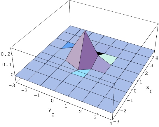
Figure 4: $f^{\scriptscriptstyle T}_{00}(x_{0},x_{1},0,0)$ on a $8\times 8$ lattice.

The FP vertex has a finite extension, i.e. it is non-negligible only on a finite set of couplings close to the origin. The couplings decay exponentially with the distance, with a characteristic length of about $0.5$ lattice units. In Fig. 4 a three-dimensional graph displays the component $f^{\scriptscriptstyle T}_{00}(x_{0},x_{1},0,0)$ on a $8\times 8$ lattice, while in Fig. 5 the exponential decay along the diagonal direction is reported. The first order vertex gives some indications about the interaction range of the full non-perturbative vertex. Our results suggest that the couplings confined inside a $2\times 2$ plaquette are the dominating ones, being those outside this region smaller than $10^{-3}$ and exponentially decaying. As a consequence, a good parametrization of the FP action should be possible with a reasonable number of terms in the lattice action.

Figure 5: Exponential decay of $|f^{\scriptscriptstyle T}_{00}(n,n,0,0)|$; the continuum line is the best fit $\sim\exp(-n/0.44)$.

5.4 The second order vertex.

The fermion propagator and the first order vertex are the only ingredients to solve the recursion relation for the second order vertex. This has a quite complicated expression, as the reader can realize by considering the formulas of Appendix C.2. It may be worthwhile to display the equation because it is independent of the particular RG transformation used, the details of which enter only through the functions $\Theta_{\mu\nu}$, $\omega_{F}$,  ${\cal E}^{\scriptscriptstyle(1)}_{\mu}$ and ${\cal E}^{\scriptscriptstyle(2)}_{\mu\nu}$, whose definition and particular expressions for our case are given in the appendices A and B. The iterative solution to the FP equation for the second order vertex is also displayed in Appendix C.2. It can be written in a concise way as

$$R^{\scriptscriptstyle(2)\,FP}_{\mu\nu}(q,q^{\prime},q^{\prime\prime})\;=\;-\,i\,\sum_{l,l^{\prime},l^{\prime\prime}=-\infty}^{\infty}\,D_{\scriptscriptstyle FP}^{-1}(q)\,\bar{J}_{\mu\nu}(\tilde{q},\tilde{q}^{\prime},\tilde{q}^{\prime\prime})\,D_{\scriptscriptstyle FP}^{-1}(-q^{\prime})$$

$$+\>\sum_{n=1}^{\infty}\,\left(\frac{1}{2}\right)^{3n-1}\,\sum_{l,l^{\prime},l^{\prime\prime}=0}^{2^{n}-1}\,D_{\scriptscriptstyle FP}^{-1}(q)\,\bar{I}^{\scriptscriptstyle(n)}_{\mu\nu}\,(\tilde{q}/2^{n},\tilde{q}^{\prime}/2^{n},\tilde{q}^{\prime\prime}/2^{n})\,D_{\scriptscriptstyle FP}^{-1}(-q^{\prime})$$

$$-\>R^{\scriptscriptstyle(1)\,FP}_{\mu}(q,-q^{\prime\prime})\,D_{\scriptscriptstyle FP}(q^{\prime\prime})\,R^{\scriptscriptstyle(1)\,FP}_{\nu}(q^{\prime\prime},q^{\prime})\,.$$ (52)

We use the notation $\tilde{q}=q+2\pi l$, $\tilde{q}^{\prime}=q^{\prime}+2\pi l^{\prime}$ and $\tilde{q}^{\prime\prime}=q^{\prime\prime}+2\pi l^{\prime\prime}$. The explicit form of the functions $\bar{J}_{\mu\nu}$ and $\bar{I}_{\mu\nu}$ is given in Appendix C.2.

The matrix structure of the vertex is the most general consistent with the symmetries. It can be written as

$$R^{\scriptscriptstyle(2)\,FP}_{\mu\nu}(q,q^{\prime},q^{\prime\prime})\;=\;\sum_{\rho}\,T_{\mu\nu\rho}(q,q^{\prime},q^{\prime\prime})\,\gamma_{\rho}\>+\>T_{\mu\nu}^{\scriptscriptstyle A}(q,q^{\prime},q^{\prime\prime})\,\gamma_{5}\>+\>T_{\mu\nu}^{\scriptscriptstyle V}(q,q^{\prime},q^{\prime\prime})\,I\,.$$ (53)

As in the case of the first order FP vertex, all the terms in the last expression turn out to be of the same order of magnitude.

Again, the sums of the first term in the r.h.s. of Eq. (52) (the one involving $\bar{J}_{\mu\nu}$) can be performed with very high precision. The third term gives no difficulty once the first order FP vertex has been computed. The second term, however, is an infinite series in $n$, the n-th summand being a sum of $2^{n}$ terms which contain very complicated functions, including the first order vertex on arbitrarily large lattices. Since the computation time grows with the sixth power of $n$, we could not go beyond $n=3$, and even in this case the computation of the complete vertex turns out to be problematic on a small lattice, due to the large number of arguments and the complicated structure of the summands. However, the perturbative evaluation of the mass gap requires the second order vertex only for a particular choice of momenta and Lorentz indices (see Eq. (55)), being as a consequence the approximate computation feasible.

The function $\bar{I}^{\scriptscriptstyle(n)}$ in Eq. (52) contains the first order vertex $R^{\scriptscriptstyle(1)}_{\mu}$ on a lattice of size $2^{n}N$, where $N$ is the size of the starting lattice. Since we are not able to calculate (at least with good precision) the first order vertex on larger lattices, we truncate its couplings to relative distances in all components $|\Delta x_{\mu}|$ smaller than four lattice units. This is a quite good approximation, since the couplings associated to distances outside this region are smaller than $10^{-4}$ (see Fig. 5). We made a numerical check of this approximation: increasing the truncation size to 6 lattice units the results for the second order vertex change by $10^{-5}$ at most.

Our crudest approximation is the truncation of the series in $n$, this time at $n=3$. In this case, we expected systematic errors of order $10^{-3}$. Again, the main danger comes from the violation of gauge invariance, and a check is given by the Ward identity:

$$\sum_{\mu}\,(\widehat{q-q^{\prime\prime}})_{\mu}\,[\,R^{\scriptscriptstyle(2)}_{\mu\nu}(q,q^{\prime}q^{\prime\prime})\>+\>R^{\scriptscriptstyle(2)}_{\nu\mu}(q,q^{\prime}q-q^{\prime}-q^{\prime\prime})\,]\;=$$

$$\hskip 113.81102ptR^{\scriptscriptstyle(1)}_{\nu}(q^{\prime\prime},q^{\prime})\>-\>R^{\scriptscriptstyle(1)}_{\nu}(q,q^{\prime}+q^{\prime\prime}-q)\,.$$ (54)

With our approximation the violations of Eq. (54) are at most of order $10^{-3}$. How this systematic error may affect the computation of the mass gap is unclear at this stage.

6 The mass gap.

In this Section we review the computation of the 1-loop mass gap with both the standard and the FP action.

The 1-loop vacuum polarization is given by

$$\Pi_{\mu\nu}(q) = \int_{BZ}\,\frac{d^{2}p}{(2\pi)^{2}}\,Tr\,\left[\,R^{\textstyle\scriptscriptstyle(1)}_{\mu}(p,q-p)\,D(p-q)\,R^{\textstyle\scriptscriptstyle(1)}_{\nu}(p-q,-p)\,D(p)\right.$$ (55)

$$+ \left.\left(\,R_{\mu\nu}^{\scriptscriptstyle(2)}(p,-p,p-q)\>+\>R_{\nu\mu}^{\scriptscriptstyle(2)}(p,-p,p+q)\,\right)\,D(p)\,\right]\,.$$

Let us now consider the numerical results. We start discussing those for the standard action. Fig. 6 represents the $11$ component of the lattice vacuum polarization $\Pi_{\mu\nu}$ at zero spatial momentum as a function of the energy $q_{0}$, for different values of the ratio $L/a$; the case $L=\infty$ is also reported. As expected from the discussion of Sec. 3.3, the cut off effects ($a$ varying with fixed $L$) show themselves as finite volume effects ($L$ varying with fixed $a$). These are large for the Wilson action; in the case $L/a=2$ the theory contains no particle at all, since the vacuum polarization has the wrong sign. The mass is obtained - according to Eq. (24) - by extrapolating the vacuum polarization to zero energy. In Fig. 7 and Table 1 we report the values of the ratio $m_{\scriptscriptstyle ph}/e$ - in the Table we report also the value of $F^{\scriptscriptstyle(1)}(a/L)$ (see Eqs. (25) and (26)) ; from these data we obtain: $m_{\scriptscriptstyle ph}/e=0.5641900+1.9\cdot(a/L)^{2}+O((a/L)^{4})$, to be compared with the continuum value $m_{\scriptscriptstyle ph}^{\scriptscriptstyle(c)}/e=0.5641896$.

Figure 6: The $11$ component of the lattice vacuum polarization $\Pi_{11}$ at zero spatial momentum as a function of the energy for various values of the ratio $L/a$ in the case of the Wilson action; the extrapolation to infinite volume (dashed line) is also reported.

Figure 7: The ratio $m_{\scriptscriptstyle ph}/e$ as a function of $a/L$ for the Wilson action (plus) and the FP action (crosses); the solid line is the continuum value $1/\sqrt{\pi}$.

$L/a$	$m_{\scriptscriptstyle ph}/e\,(Wil)$	$F^{(1)}\,(Wil)$	$m_{\scriptscriptstyle ph}/e\,(FP)$	$F^{(1)}\,(FP)$
2			0.577989475	0.013800
4	0.3528	-0.21132	0.565117686	0.000928
6	0.49158	-0.07260	0.564524513	0.000335
8	0.52924	-0.03495	0.564434047	0.000244
16	0.55668	-0.00751
32	0.56236	-0.00183
64	0.56373	-0.00045
128	0.56407	-0.00011
256	0.56416	-0.00003
$\infty$	0.5641900		0.564335184

Table 1: the values of $m_{\scriptscriptstyle ph}/e$ and $F^{(1)}$ for the Wilson and FP action

In the case of the FP action we observe a radically different behavior. In Fig. 8 we show the vacuum polarization in the infinite volume case, together with the same quantity in the case $L/a=4$ for some values of the energy: we observe only tiny finite volume effects, probably due to our numerical approximations. The cut off effects in the lattice mass gap are directly related to the finite volume effects of the lattice vacuum polarization only for $q_{0}=0$. The absence of finite volume effects even for non-zero values of the energy with the FP action is in this sense an extra bonus. We verified that the volume-independence of the zero spatial momentum vacuum polarization is indeed a property of the continuum theory, probably related to the fact that the real underlying theory of the Schwinger model is a free-field scalar theory.

In Fig. 7 and Table 1 we report the results for mass gap with the FP action. Except for the case $L/a=2$, which requires a particular discussion, we see very small deviations from the continuum, of order of the numerical errors in the determination of the fixed point vertices ($10^{-3}\div 10^{-4}$). We remark that these deviations cannot be considered pure cut off effects, since they are in part produced by a violation of the gauge symmetry. Indeed, a deviation from the correct continuum value of order $10^{-4}$ is observed even in the infinite volume case, where in principle no cut off effects are present for any action. The large deviation from the continuum for $L/a=2$ is related to an additional effect [14] exponentially decaying with increasing $L/a$ and related to the finite extension of the FP action.

Figure 8: The $11$ component of the lattice vacuum polarization $\Pi_{11}$ in the infinite volume (dashed line) and for $L/a=4$ (crosses) in the case of the FP action.

7 The 1-loop perfection of the FP action.

The results of the last Section are consistent with a picture of no power-like cut off effects for the 1-loop mass gap in the case of the FP action. The point is now whether this outcome can be interpreted as an effect of a (hypothetical) 1-loop quantum perfection of the FP action of the Schwinger model - we recall that any FP action is by construction perfect only at the classical level.

The definition of quantum perfection is related to the behavior of the action under RG transformations at finite values of $\beta$. We recall the form of the FP action:

$$S^{\scriptscriptstyle FP}\;=\;\beta\,S_{g}^{\scriptscriptstyle FP}(A)\>+\>\bar{\psi}\,\Delta^{\scriptscriptstyle FP}(U)\,\psi\,.$$ (56)

After one RG transformation the action $S^{\scriptscriptstyle FP}$ changes into $S^{\prime}$:

$$S^{\prime}\;=\;\frac{\beta}{4}\,(\,S_{g}^{\scriptscriptstyle FP}(A)\>+\>\delta S_{g}(A)\,)\>+\>\bar{\psi}\,\Delta^{\scriptscriptstyle FP}(U)\,\psi\>+\>\delta S_{\scriptscriptstyle F}(\bar{\psi},\psi,U)\;.$$ (57)

The corrections $\delta S_{g}$ and $\delta S_{\scriptscriptstyle F}$ have a perturbative expansion in $g$, the leading term being $O(g^{2})$; in particular, the fermion correction contains four-fermions interactions. The 1-loop quantum perfection means the absence of the leading terms in the perturbative expansion of $\delta S_{g}$ and $\delta S_{\scriptscriptstyle F}$. The absence of cut off effects in the mass gap for the FP action requires a weaker property. The 1-loop mass gap in units of the charge is a non-universal function of $a/L$; denoting with a prime the quantities relative to the action $S^{\prime}$ of Eq. (57), we have:

$$m^{\scriptscriptstyle FP}_{\scriptscriptstyle ph}/e\;=\;F^{\scriptscriptstyle FP}(a/L)\,,\hskip 28.45274ptm^{\prime}_{\scriptscriptstyle ph}/e\;=\;F^{\prime}(a/L)\;.$$ (58)

The mass-charge ratio, being the dimensionless ratio of physical quantities, does not change after a RG transformation. Hence:

$$F^{\scriptscriptstyle FP}(a/L)\;=\;F^{\prime}(2\,a/L)\;=\;F^{\scriptscriptstyle FP}(2\,a/L)\>+\>\delta F^{\prime}(2\,a/L)\;.$$ (59)

The last equality is suggested by Eq. (57). The correction $\delta F^{\prime}$ comes from the leading terms in the perturbative expansion of $\delta S_{g}$ and $\delta S_{\scriptscriptstyle F}$; absence of cut off effects for the FP action means $\delta F^{\prime}=0$, since we see from Eq. (59) that $F^{\scriptscriptstyle FP}$ is in this case independent from $a/L$. After inspecting all the possible vertices generated by the RG transformation, one concludes that the only term which can contribute at 1-loop is a tree level term, quadratic in the field $A_{\mu}$. Gauge invariance implies (in two dimensions) the form:

$$\sum_{\mu\nu}\,A_{\mu}(q)^{*}\,C(q)\,\left(\,\left|\hat{q}\right|^{2}\,\delta_{\mu\nu}\>-\>\hat{q}_{\mu}\,\hat{q}_{\nu}^{*}\,\right)\,A_{\nu}(q)\,,$$ (60)

where $C(q)$ is some regular function of $q$. This term gives no contribution to the mass gap, since it vanishes at $q=0$. As a consequence, $\delta F^{\prime}\,=\,0$.

The previous discussion shows that the absence of cut off effects in the 1-loop mass gap is indeed an effect of the classical perfection of the FP action. This is a non trivial point, since a formal argument [18, 4] of the RG implies the 1-loop quantum perfection of the FP action. This argument has been recently disproved by Hasenfratz and Niedermayer [15] by the explicit determination in perturbation theory of the 1-loop quantum perfect action of the $O(3)-\sigma$ model. We do not expect something different for the Schwinger model, although, due to the different nature of the lagrangian (gauge interactions between two fields instead of self-interactions) we think it would be worthwhile to repeat the check even in the present case. Another important point would be to understand where the formal argument of the RG breaks down.

8 Conclusions.

Let us briefly summarize the results and the conclusions of this work. We have obtained perturbatively the FP action of the Schwinger model for a particular RG transformation. Using the non-compact formulation, we could solve analytically the pure gauge part. In this way we could concentrate the numerical effort to the fermion sector, which was treated perturbatively.

The photon-fermion first order vertex turns out to have couplings exponentially decaying with the distance, as expected from RG arguments. The most important ones are those connecting first and second neighbors. We expect from this observation that a good approximation of the FP action can be obtained with a simple parametrization containing only short-ranged couplings.

The perfection of the FP action has been shown by computing the mass gap at finite spatial volume. We found big cut off effects with the standard action, and negligible with the FP action. Contrarily to what can be naively inferred, the calculation of the mass gap represents a check of the classical - tree level - perfection, and not of the 1-loop quantum perfection; this latter property can be checked [15] by computing higher excited states in the spectrum.

Acknowledgments

We are indebted with P. Hasenfratz and F. Niedermayer for having introduced us in the subject and for useful suggestions. We acknowledge valuable discussions with C.B. Lang and T.K. Pany. The work received financial support from Fondazione “A. Della Riccia”- Italy (F.F.) and Ministerio de Educación y Cultura - Spain under grant PF-95-73193582 (V.L.).

A Appendix.

In this Appendix we give some details about the solution of the recursion relation for the free gauge field. We follow the ideas of [4], and we refer to this paper for further details.

A.1 The FP pure gauge propagator.

In this part we give some hints about the algebraic manipulations which lead to the pure gauge FP propagator, Eq. (29). We write the general formulas for an arbitrary dimension $d$, specializing at the end the solutions to $d=2$.

Consider the RG kernel:

$${\cal K}_{g}(A^{\prime},A)\;=\;\sum_{x_{B}\,\mu}\,\left(\,A^{\prime}_{\mu}(x_{B})\,-\,\sum_{x\,\nu}\,\omega_{\mu\nu}(2x_{B}-x)\,A_{\nu}(x)\,\right)^{2}\,.$$ (A.1)

In the case of the transformation of Eq. (28), generalized to arbitrary dimensions, $\omega_{\mu\nu}$ is written:

$$\omega_{\mu\nu}(2x_{B}-x)\;=\;2^{d_{A}-1}\,\delta_{\mu\nu}\,\left(\,\delta_{2x_{B}\,,\,x}\>+\>\delta_{2x_{B}+\hat{\mu}\,,\,x}\,\right)\,,$$ (A.2)

where $d_{A}=(d-2)/2$ is the dimension of the gauge field. In Fourier space the last formula reads:

$$\omega_{\mu\nu}(q)\;=\;\sum_{x}\,e^{-iqx}\,\omega_{\mu\nu}(x)\;=\;2^{d_{A}-1}\,\left(\,1\,+\,e^{iq_{\mu}}\,\right)\,\delta_{\mu\nu}\,.$$ (A.3)

Since the original action and the RG kernel are quadratic in the gauge field, the coarse action is also quadratic. From gaussian integration we obtain a recursion relation which relates the coarse and fine propagators [4]:

$$G^{\prime}_{\mu\nu}(q)\;=\;2^{-d}\,\sum_{l=0}^{1}\,\sum_{\rho\sigma}\,\omega_{\mu\rho}(\frac{q+2\pi l}{2})\,G_{\rho\sigma}(\frac{q+2\pi l}{2})\,\omega^{\dagger}_{\sigma\nu}(\frac{q+2\pi l}{2})\>+\>\frac{1}{\kappa_{g}}\,\delta_{\mu\nu}\,.$$ (A.4)

After $n$ iterations of the recursion relation one gets

$$G^{\scriptscriptstyle(n)}_{\mu\nu}(q) = 2^{(2d_{A}-d)n}\,\sum_{l=0}^{2^{n}-1}\,\sum_{\rho\sigma}\,\Omega^{\scriptscriptstyle(n)}_{\mu\rho}(\frac{q+2\pi l}{2^{n}})\,G^{\scriptscriptstyle(0)}_{\rho\sigma}(\frac{q+2\pi l}{2^{n}})\,\Omega^{{\scriptscriptstyle(n)}\,\dagger}_{\sigma\nu}(\frac{q+2\pi l}{2^{n}})$$ (A.5)

$$+ \frac{1}{\kappa_{g}}\,\sum_{j=0}^{n-1}\,2^{(2d_{A}-d)j}\,\sum_{l=0}^{2^{j}-1}\,\sum_{\rho}\,\Omega^{\scriptscriptstyle(j)}_{\mu\rho}(\frac{q+2\pi l}{2^{j}})\ \Omega^{{\scriptscriptstyle(j)}\,\dagger}_{\rho\nu}(\frac{q+2\pi l}{2^{j}})\,,$$

where

$$\Omega^{\scriptscriptstyle(j)}_{\mu\nu}(\frac{q+2\pi l}{2^{j}})\;=\;2^{-d_{A}j}\,\left[\,\omega(\frac{q+2\pi l}{2})\,\omega(\frac{q+2\pi l}{2^{2}})\ldots\omega(\frac{q+2\pi l}{2^{j}})\,\right]_{\mu\nu}$$ (A.6)

and

$$\Omega^{\scriptscriptstyle(0)}_{\mu\nu}(q+2\pi l)\;=\;\delta_{\mu\nu}\,.$$ (A.7)

In our case (Eq. (A.3)) the result is:

$$\Omega^{\scriptscriptstyle(j)}_{\mu\nu}(\frac{q+2\pi l}{2^{j}})\;=\;2^{-j}\,\frac{e^{iq_{\mu}}-1}{\exp(i\frac{q_{\mu}+2\pi l_{\mu}}{2^{j}})-1}\,\delta_{\mu\nu}\ .$$ (A.8)

The FP propagator is obtained by inserting this last expression into Eq. (A.5) and taking the $n\rightarrow\infty$ limit. In the r.h.s. of Eq. (A.5), only the modes with $\frac{q+2\pi l}{2^{n}}\sim\frac{1}{2^{n}}$ contribute to the homogeneous part (the one containing $G_{\mu\nu}^{(0)}$); the inhomogeneous term (proportional to $\kappa_{g}^{-1}$) is easily calculated by making use of following formula, valid for one-dimensional summation:

$$\sum_{j=0}^{2^{n}-1}\,\frac{1}{4\,\sin^{2}(\frac{q+2\pi j}{2^{n+1}})}\;=\;\frac{2^{2n}}{4\sin^{2}(q/2)}\,.$$ (A.9)

The result for the FP propagator is, in two dimensions:

$$G_{\mu\nu}^{\scriptscriptstyle FP}(q)\;=\;\left(\,f_{\mu}(q)\>+\>\frac{2}{\kappa_{g}}\,\right)\,\delta_{\mu\nu}\;+\;(\xi^{-1}\,-\,1)\,g(q)\,\hat{q}_{\mu}\,\hat{q}_{\nu}^{*}\,,$$ (A.10)

where

$$f_{\mu}(q) = \left|\,\hat{q}_{\mu}\,\right|^{2}\,\sum_{l=-\infty}^{+\infty}\,\frac{1}{\left(q_{\mu}+2\pi\,l_{\mu}\right)^{2}}\,\frac{1}{\left(q+2\pi\,l\right)^{2}}$$

$$g(q) = \sum_{l=-\infty}^{+\infty}\,\frac{1}{\left(q+2\pi\,l\right)^{4}}\,.$$ (A.11)

A.2 The connecting tensor.

According to the discussion of Section 2, in order to solve the problem of the interaction between gauge field and fermions, we need the fine configuration minimizing the r.h.s. of Eq. (4) as a function of the coarse configuration $A^{\prime}$. Since both the fine action and the gauge kernel are quadratic, the relation is linear:

$$A_{\mu}^{min}(\frac{q+2\pi\,l}{2})\;=\;\sum_{\nu}\,Z_{\mu\nu}(\frac{q+2\pi\,l}{2})\,A_{\nu}^{\prime}(q)\,,$$ (A.12)

where $l_{\mu}=0,1$. In ref. [4] is shown that

$$Z_{\mu\nu}(\frac{q+2\pi l}{2})\;=\;\sum_{\rho\sigma}\,G^{\scriptscriptstyle FP}_{\mu\rho}(\frac{q+2\pi l}{2})\,\omega_{\rho\sigma}^{\dagger}(\frac{q+2\pi l}{2})\,G^{{\scriptscriptstyle FP}\,-1}_{\sigma\nu}(q)\ .$$ (A.13)

In the iterative solution of the recursion relations for the vertices, some products of $Z_{\mu\nu}$ appear. Since these products have always the same form, it is useful to define

$$\Theta^{\scriptscriptstyle(n)}_{\mu\nu}(q/2^{n})\;=\;2^{-(d_{A}+2)n}\,\sum_{\rho_{1}\ldots\rho_{n-1}}\,Z_{\mu\rho_{1}}(\frac{q}{2^{n}})\,Z_{\rho_{1}\rho_{2}}(\frac{q}{2^{n-1}})\,\cdots\,Z_{\rho_{n-1}\nu}(\frac{q}{2})\,.$$ (A.14)

Particularizing to our transformation and fixing $d=2$, $Z_{\mu\nu}$ and $\Theta_{\mu\nu}^{\scriptscriptstyle(n)}$ read:

$$Z_{00}(q) = \frac{1}{2}\,\left(\,1\,+\,e^{-iq_{1}}\,\right)\,\left[\,\left|\hat{q}_{0}\right|^{2}\,\frac{g(q)}{g(2q)}\,f_{1}(2q)\>+\>\left|\widehat{2q_{1}}\right|^{2}\,f_{0}(q)\,\right]$$

$$Z_{01}(q) = \frac{1}{2}\,\hat{q}_{0}\,\widehat{2q}_{2}^{*}\,\left[\,\frac{g(q)}{g(2q)}\,f_{0}(2q)\>-\>f_{0}(q)\,\frac{\left|\widehat{2q}_{0}\right|^{2}}{\left|\hat{q}_{0}\right|^{2}}\,\right]\,,$$ (A.15)

and

$$\Theta^{\scriptscriptstyle(n)}_{00}(q/2^{n}) = \frac{1}{8^{n}}\,\frac{\hat{q}_{0}^{*}}{\widehat{(q_{0}/2^{n})}^{*}}\,\left[\,|\hat{q}_{1}|^{2}\,f_{0}(q/2^{n})\>+\>\left|\widehat{(q_{0}/2^{n})}\right|^{2}\,\frac{g(q/2^{n})}{g(q)}\,f_{1}(q)\,\right]$$

$$\Theta^{\scriptscriptstyle(n)}_{01}(q/2^{n}) = \frac{1}{8^{n}}\,\frac{\hat{q}_{1}^{*}}{\widehat{(q_{0}/2^{n})}^{*}}\,\left[\,\left|\widehat{(q_{0}/2^{n})}\right|^{2}\,\frac{g(q/2^{n})}{g(q)}\,f_{0}(q)\>-\>|\hat{q}_{0}|^{2}f_{0}(q/2^{n})\,\right]\,.$$

(A.16)

The remaining components can be obtained from these by properly changing $0\leftrightarrow 1$.

When $n\rightarrow\infty$, keeping $q$ fixed, we obtain:

$$\Theta^{\scriptscriptstyle(\infty)}_{00}(q) = i\,\frac{\hat{q}_{0}^{*}}{q_{0}}\,\left(\,\frac{|\hat{q}_{1}|^{2}}{q^{2}}\>+\>\frac{q_{0}^{2}}{q^{4}}\,\frac{f_{1}(q)}{g(q)}\,\right)$$

$$\Theta^{\scriptscriptstyle(\infty)}_{01}(q) = i\,\frac{\hat{q}_{1}^{*}}{q_{0}}\,\left(\,\frac{q_{0}^{2}}{q^{4}}\,\frac{f_{0}(q)}{g(q)}\>-\>\frac{|\hat{q}_{0}|^{2}}{q^{2}}\,\right)\,.$$ (A.17)

These expressions appear in the solution of the recursion relations for the first and second order vertices, as given in Appendix C.

B Appendix.

In this Appendix we give some details concerning the fermion RG transformation. We start with some relations concerning the free fermion problem wich are relevant for the computation of the FP vertices. In a second part we work out the fermion kernel in presence of the interaction with a $U(1)$ gauge field.

B.1 Formulas for the free fermion problem.

The free fermion kernel is defined through a function $\omega_{F}$

$$\Gamma^{0}(x_{B})\;=\;\sum_{x}\,\omega_{F}(2x_{B}-x)\,\psi_{x}\,.$$ (B.1)

The RG transformation of Sec. 5.1 reads in arbitrary dimensions:

$$\Gamma^{0}(x_{B}) = 2^{d_{\psi}-d}\,\left[\,\psi(2x_{B})\>+\>\frac{1}{2}\,\sum_{\mu}\>\sum_{\lambda=\pm 1}\,\psi(2x_{B}\,+\,\lambda\hat{\mu})\right.$$ (B.2)

$$+ \frac{1}{4}\,\sum_{\mu<\nu}\>\sum_{\lambda_{\mu}=\pm 1}\>\sum_{\lambda_{\nu}=\pm 1}\,\psi(2x_{B}\,+\,\lambda_{\mu}\hat{\mu}\,+\,\lambda_{\nu}\hat{\nu})$$

$$+ \left.\cdots+\frac{1}{2^{d}}\,\sum_{\lambda_{1}=\pm 1}\cdots\sum_{\lambda_{d}=\pm 1}\,\psi(2x_{B}\,+\,\lambda_{1}\hat{1}\,+\cdots\,\lambda_{d}\hat{d})\,\right]\,,$$

where $d_{\psi}=(d-1)/2$ is the dimension of the fermion field. In Fourier transform:

$$\omega_{F}(q)\;=\;2^{d_{\psi}}\prod_{\mu}\,\cos^{2}\frac{q_{\mu}}{2}\,.$$ (B.3)

For the iterative solution of the FP equations, it is useful to define a new function, analogous to $\Omega^{\scriptscriptstyle(n)}_{\mu\nu}$ of the pure gauge problem:

$$\Omega^{\scriptscriptstyle(n)}_{F}(q/2^{n})\;=\;2^{-d_{\psi}\,n}\,\omega_{F}(q/2)\,\omega_{F}(q/2^{2})\,\cdots\,\omega_{F}(q/2^{n})\,.$$ (B.4)

In the case of the transformation (B.2):

$$\Omega^{\scriptscriptstyle(n)}_{F}(q/2^{n})\;=\;\prod_{\mu}2^{-2n}\,\frac{\sin^{2}(q_{\mu}/2)}{\sin^{2}(q_{\mu}/2^{n+1})}\,.$$ (B.5)

Using (mutatis mutandis) Eq. (A.5) one arrives, in two dimensions, to the result of Eqs. (42) and (5.1).

B.2 The fermion gauge invariant kernel.

In this part we shall write down some formulas concerning the fermion kernel in presence of gauge interactions. In order to keep the coarse action gauge invariant, we define a gauge covariant average procedure for the fermion fields defined on the original fine lattice. This is achieved by parallel transporting the fine fields to the coarse site to which they contribute. We choose the simplest symmetric paths which join $x_{B}$ with its neighbors to make (B.2) gauge covariant (we write the formulas directly for the case $d=2$):

$$\Gamma(x_{B};\,U)\;=\;\frac{\sqrt{2}}{4}\,\left\{\,\psi(2x_{B})\>+\>\frac{1}{2}\,\Gamma_{fn}(x_{B};\,U)\>+\>\frac{1}{4}\,\Gamma_{dn}(x_{B};\,U)\,\right\}\,,$$ (B.6)

where $\Gamma_{fn}$ and $\Gamma_{dn}$ stand for the contribution of the first and diagonal neighbors respectively, and are built from the paths depicted in Fig. 3. The expression for them are:

$$\Gamma_{fn}(x_{B};\,U) = U_{0}(2x_{B})\psi(2x_{B}+\hat{0})\,+\,U_{0}^{\dagger}(2x_{B}-\hat{0})\,\psi(2x_{B}-\hat{0})$$

$$+ U_{1}(2x_{B})\psi(2x_{B}+\hat{1})\,+\,U_{1}^{\dagger}(2x_{B}-\hat{1})\,\psi(2x_{B}-\hat{1})\,.$$

and

$$\Gamma_{dn}(x_{B};\,U)\;=$$ (B.8)

$$\left[\,U_{0}(2x_{B})U_{1}(2x_{B}+\hat{0})\,+\,U_{1}(2x_{B})U_{0}(2x_{B}+\hat{1})\,\right]\,\psi(2x_{B}+\hat{0}+\hat{1})\>+$$

$$+ \left[\,U_{0}(2x_{B})U_{1}^{\dagger}(2x_{B}+\hat{0}-\hat{1})\,+\,U_{1}^{\dagger}(2x_{B}-\hat{1})U_{0}(2x_{B}-\hat{1})\,\right]\,\psi(2x_{B}+\hat{0}-\hat{1})$$

$$+ \left[\,U_{0}^{\dagger}(2x_{B}-\hat{0})U_{1}(2x_{B}-\hat{0})\,+\,U_{1}(2x_{B})U_{0}^{\dagger}(2x_{B}-\hat{0}+\hat{1})\,\right]\,\psi(2x_{B}-\hat{0}+\hat{1})\$$

$$+ \left[U_{0}^{\dagger}(2x_{B}-\hat{0})U_{1}^{\dagger}(2x_{B}-\hat{0}-\hat{1})+U_{1}^{\dagger}(2x_{B}-\hat{1})U_{0}^{\dagger}(2x_{B}-\hat{0}-\hat{1})\right]\times$$

$$\;\;\;\;\;\;\;\;\;\;\;\;\;\;\;\;\;\;\;\;\;\;\;\;\;\;\;\;\;\;\;\;\;\;\;\;\;\;\;\;\;\;\;\;\;\;\;\;\;\;\;\;\;\;\;\;\;\;\;\;\;\;\;\;\;\;\;\;\;\;\;\;\psi(2x_{B}-\hat{0}-\hat{1})\,.$$

Expanding $U_{\mu}$ in powers of $A_{\mu}$ we obtain:

$$\Gamma(x_{B};\,U(A)) = \Gamma^{0}(x_{B})\>+\>i\,\sum_{x\,r}\,\sum_{\mu}\,A_{\mu}(r)\,{\cal E}^{\scriptscriptstyle(1)}_{\mu}(2x_{B}-r,x-r)\,\psi_{x}$$

$$+ \sum_{x\,r\,r^{\prime}}\,\sum_{\mu\nu}\,A_{\mu}(r)\,A_{\nu}(r^{\prime})\,{\cal E}^{\scriptscriptstyle(2)}_{\mu\nu}(2x_{B}-r,x-r^{\prime},r-r^{\prime})\,\psi_{x}\,+\,O(A^{3})\,.$$

In momentum space ${\cal E}^{\scriptscriptstyle(1)}_{\mu}$ and ${\cal E}^{\scriptscriptstyle(2)}_{\mu\nu}$ read:

$${\cal E}^{\scriptscriptstyle(1)}_{0}(q,q^{\prime})\;=\;\frac{\sqrt{2}}{8}\,\left(\,\hat{q^{\prime}}_{0}^{*}\>-\>\hat{q}_{0}^{*}\,\right)\,\left(1\>+\>\frac{\cos q_{1}\,+\,\cos q^{\prime}_{1}}{2}\,\right)$$ (B.10)

and

$${\cal E}^{\scriptscriptstyle(2)}_{00}(q,q^{\prime},q^{\prime\prime}) = -\,\frac{\sqrt{2}}{16}\,\left(\,e^{-iq_{0}}\>+\>e^{-iq_{0}^{\prime}}\,\right)\,\left(1\>+\>\frac{\cos q_{1}\,+\,\cos q_{1}^{\prime}}{2}\,\right)$$

$${\cal E}^{\scriptscriptstyle(2)}_{01}(q,q^{\prime},q^{\prime\prime}) = \frac{\sqrt{2}}{16}\,\exp(-i\frac{q_{0}-q_{0}^{\prime\prime}}{2})\,\exp(-i\frac{q_{1}^{\prime}+q_{1}^{\prime\prime}}{2})\times$$

$$\hskip 14.22636pt\left(\sin\frac{q_{0}+q_{0}^{\prime\prime}}{2}\sin\frac{q_{1}^{\prime\prime}-q_{1}^{\prime}}{2}\,-\,\sin(q_{0}^{\prime}-\frac{q_{0}-q_{0}^{\prime\prime}}{2})\sin(q_{1}-\frac{q_{1}^{\prime}+q_{1}^{\prime\prime}}{2})\right)\,.$$ (B.11)

The remaining components can be obtained as usual by properly changing $0\leftrightarrow 1$.

C Appendix.

In this Appendix we write down the equations relative to the RG iteration relation for the first and second order vertex. They are the result of a long but straightforward calculation.

C.1 Recursion relation for the first order vertex.

In order to simplify the expressions, we use the notation $\tilde{q}=q+2\pi l$ and $\tilde{q^{\prime}}=q^{\prime}+2\pi l^{\prime}$. The recursion relation verified by the first order vertex is:

$$R_{\mu}^{{\scriptscriptstyle(1)}\,\prime}(q,-q^{\prime}) = D_{\scriptscriptstyle FP}^{-1}(q)\,\left(\frac{1}{2}\right)^{2d}\,\sum_{l,l^{\prime}=0}^{1}\,\sum_{\nu}\,Z_{\nu\mu}(\frac{\tilde{q}-\tilde{q}^{\prime}}{2})\,\times$$ (C.1)

$$\left[\,H_{\nu}(\tilde{q}/2,\,\tilde{q}^{\prime}/2)\>+\>X_{\nu}(\tilde{q}/2,\,\tilde{q}^{\prime}/2)\,\right]\,D_{\scriptscriptstyle FP}^{-1}(q^{\prime})\,,$$

where

$$H_{\nu}(k,k^{\prime})\;=\;\omega_{F}(k)\,D_{\scriptscriptstyle FP}(k)\,R^{\scriptscriptstyle(1)}_{\nu}(k,\,-k^{\prime})\,D_{\scriptscriptstyle FP}(k^{\prime})\,\omega_{F}^{\dagger}(k^{\prime})$$ (C.2)

and

$$X_{\nu}(k,k^{\prime})\;=\;\omega_{F}(k)\,D_{\scriptscriptstyle FP}(k)\,{\cal E}^{{\scriptscriptstyle(1)}\,\dagger}_{\nu}(k^{\prime},\,-k)\>-\>{\cal E}^{\scriptscriptstyle(1)}_{\nu}(k,\,-k^{\prime})\,D_{\scriptscriptstyle FP}(k^{\prime})\,\omega_{F}^{\dagger}(k^{\prime})\,.$$ (C.3)

We point out that this formula holds formally for arbitrary dimensions and gauge groups.

We now specialize derivation to the case of the Schwinger model. In this case a factor-two renormalization of the gauge field is required (see the discussion of Sec. 5.3). The recursion relation (C.1) leads to the FP vertex:

$$R^{\scriptscriptstyle FP\,(1)}_{\mu}(q,-q^{\prime})\;=\;\sum_{l,l^{\prime}=-\infty}^{+\infty}\,\overline{H}_{\mu}(q,q^{\prime},l,l^{\prime})\>+\>\sum_{n=1}^{\infty}\,\frac{1}{4^{n}}\,\sum_{l,l^{\prime}=0}^{2^{n}-1}\,\overline{X}^{\scriptscriptstyle(n)}_{\mu}(q,q^{\prime},l,l^{\prime})\,,$$ (C.4)

where

$$\overline{H}_{\mu}(q,q^{\prime},l,l^{\prime})\;=\;-\,D_{\scriptscriptstyle FP}^{-1}(q)\,\sum_{\rho\beta\omega}\,\Theta^{\scriptscriptstyle(\infty)}_{\rho\mu}(\tilde{q}-\tilde{q}^{\prime})\,\frac{\tilde{q}_{\beta}\,\tilde{q}^{\prime}_{\omega}}{\tilde{q}^{2}\,\tilde{q}^{\prime\,2}}\,\gamma_{\beta}\,\gamma_{\rho}\,\gamma_{\omega}\,D_{\scriptscriptstyle FP}^{-1}(q^{\prime})\,\times$$

$$\hskip 113.81102pt\prod_{\alpha}\,\frac{16\sin^{2}(q_{\alpha}/2)\sin^{2}(q^{\prime}_{\alpha}/2)}{\tilde{q}_{\alpha}^{2}\,\tilde{q}_{\alpha}^{\prime\,2}}$$ (C.5)

and

$$\overline{X}^{\scriptscriptstyle(n)}_{\mu}(q,q^{\prime},l,l^{\prime})\;=\;\frac{1}{\sqrt{2}}\,D_{\scriptscriptstyle FP}^{-1}(q)\,\sum_{\rho}\,\Theta_{\rho\mu}^{\scriptscriptstyle(n)}(\frac{\tilde{q}-\tilde{q}^{\prime}}{2^{n}})\times$$

$$\left[\,\Omega_{F}^{\scriptscriptstyle(n)}(\tilde{q}/2^{n})\,D_{\scriptscriptstyle FP}(\tilde{q}/2^{n})\,{\cal E}^{{\scriptscriptstyle(1)}\,\dagger}_{\rho}(\tilde{q}^{\prime}/2^{n}\,,\,-\tilde{q}/2^{n})\,\Omega_{F}^{{\scriptscriptstyle(n-1)}\,\dagger}(\tilde{q^{\prime}}/2^{n-1})\,\>-\right.$$

$$\left.\Omega_{F}^{\scriptscriptstyle(n-1)}(\tilde{q}/2^{n-1})\,{\cal E}^{\scriptscriptstyle(1)}_{\rho}(\tilde{q}/2^{n}\,,\,-\tilde{q}^{\prime}/2^{n})\,D_{\scriptscriptstyle FP}(\tilde{q}^{\prime}/2^{n})\,\Omega_{F}^{{\scriptscriptstyle(n)}\,\dagger}(\tilde{q}^{\prime}/2^{n})\,\right]\,D_{\scriptscriptstyle FP}^{-1}(q^{\prime})\,.$$ (C.6)

C.2 Recursion relation for the second order vertex.

The recursion relation for the second order vertex is much more complicated, and it involves the FP first order vertex:

$$R_{\mu\nu}^{{\scriptscriptstyle(2)}\,\prime}(q,q^{\prime},q^{\prime\prime})\;=\;\frac{1}{2^{3d}}\,\sum_{l,l^{\prime},l^{\prime\prime}=0}^{1}\,\sum_{\rho\sigma}\,\left\{\,D_{\scriptscriptstyle FP}^{-1}(q)\right.\,Z_{\rho\mu}(\frac{\tilde{q}-\tilde{q}^{\prime\prime}}{2})\,Z_{\sigma\nu}(\frac{\tilde{q}^{\prime}+\tilde{q}^{\prime\prime}}{2})\,\times$$

$$\hskip 28.45274pt\left.\left[\,J_{\rho\sigma}(\tilde{q}/2,\tilde{q}^{\prime}/2,\tilde{q}^{\prime\prime}/2)\;+\;I_{\rho\sigma}(\tilde{q}/2,\tilde{q}^{\prime}/2,\tilde{q}^{\prime\prime}/2)\,\right]\,D_{\scriptscriptstyle FP}^{-1}(-q^{\prime})\,\right\}$$

$$\hskip 28.45274pt-\>R^{\scriptscriptstyle(1)\,FP}_{\mu}(q,-q^{\prime\prime})\,D_{\scriptscriptstyle FP}(q^{\prime\prime})\,R^{\scriptscriptstyle(1)\,FP}_{\nu}(q^{\prime\prime},q^{\prime})\;,$$ (C.7)

where the functions $H_{\rho\sigma}$ and $I_{\rho\sigma}$ are:

$$J_{\rho\sigma}(k,k^{\prime},k^{\prime\prime})\;=\;\omega_{F}(k)\,D_{\scriptscriptstyle FP}(k)\,R_{\rho\sigma}^{\scriptscriptstyle(2)}(k,k^{\prime},k^{\prime\prime})\,D_{\scriptscriptstyle FP}(-k^{\prime})\,\omega_{F}^{\dagger}(-k^{\prime})$$ (C.8)

and

$$I_{\rho\sigma}(k,k^{\prime},k^{\prime\prime})\;=$$

$$-\>{\cal E}^{\scriptscriptstyle(2)}_{\rho\sigma}(k,k^{\prime},k^{\prime\prime})\,D_{\scriptscriptstyle FP}(-k^{\prime})\,\omega_{F}^{\dagger}(-k^{\prime})\>-\>\omega_{F}(k)\,D_{\scriptscriptstyle FP}(k)\,{\cal E}^{{\scriptscriptstyle(2)}\,\dagger}_{\rho\sigma}(-k,-k^{\prime},-k^{\prime\prime})$$

$$+\>\omega_{F}(k)\,D_{\scriptscriptstyle FP}(k)\,R^{\scriptscriptstyle(1)\,FP}_{\rho}(k,-k^{\prime\prime})\,D_{\scriptscriptstyle FP}(k^{\prime\prime})\,R^{\scriptscriptstyle(1)\,FP}_{\sigma}(k^{\prime\prime},k^{\prime})\,D_{\scriptscriptstyle FP}(-k^{\prime})\,\omega_{F}^{\dagger}(-k^{\prime})$$

$$+\>\omega_{F}(k)\,D_{\scriptscriptstyle FP}(k)\,R^{\scriptscriptstyle(1)\,FP}_{\rho}(k,-k^{\prime\prime})\,D_{\scriptscriptstyle FP}(k^{\prime\prime})\,{\cal E}^{{\scriptscriptstyle(1)}\,\dagger}_{\sigma}(-k^{\prime},-k^{\prime\prime})$$

$$-\>{\cal E}^{\scriptscriptstyle(1)}_{\rho}(k,-k^{\prime\prime})\,D_{\scriptscriptstyle FP}(k^{\prime\prime})\,R^{\scriptscriptstyle(1)\,FP}_{\sigma}(k^{\prime\prime},k^{\prime})\,D_{\scriptscriptstyle FP}(-k^{\prime})\,\omega_{F}^{\dagger}(-k^{\prime})$$

$$-\>{\cal E}^{\scriptscriptstyle(1)}_{\rho}(k,-k^{\prime\prime})\,D_{\scriptscriptstyle FP}(k^{\prime\prime})\,{\cal E}^{{\scriptscriptstyle(1)}\,\dagger}_{\sigma}(-k^{\prime},-k^{\prime\prime})\,.$$ (C.9)

The FP of the above displayed recursion relation is (taking again into account the factor-two renormalization of the gauge field):

$$R^{\scriptscriptstyle(2)\,FP}_{\mu\nu}(q,q^{\prime},q^{\prime\prime})\;=\;-\,i\,\sum_{l,l^{\prime},l^{\prime\prime}=-\infty}^{+\infty}\,D_{\scriptscriptstyle FP}^{-1}(q)\,\bar{J}_{\mu\nu}(\tilde{q},\tilde{q}^{\prime},\tilde{q}^{\prime\prime})\,D_{\scriptscriptstyle FP}^{-1}(-q^{\prime})$$

$$+\>\sum_{n=1}^{+\infty}\,\left(\frac{1}{2}\right)^{3n-1}\,\sum_{l,l^{\prime},l^{\prime\prime}=0}^{2^{n}-1}\,D_{\scriptscriptstyle FP}^{-1}(q)\,\bar{I}^{\scriptscriptstyle(n)}_{\mu\nu}\,(\tilde{q}/2^{n},\tilde{q}^{\prime}/2^{n},\tilde{q}^{\prime\prime}/2^{n})\,D_{\scriptscriptstyle FP}^{-1}(-q^{\prime})$$

$$-\>R^{\scriptscriptstyle(1)\,FP}_{\mu}(q,-q^{\prime\prime})\,D_{\scriptscriptstyle FP}(q^{\prime\prime})\,R^{\scriptscriptstyle(1)\,FP}_{\nu}(q^{\prime\prime},q^{\prime})\,,$$ (C.10)

where

$$\bar{J}_{\mu\nu}(k,k^{\prime},k^{\prime\prime})\;=\;\sum_{\rho\sigma}\,\Theta^{\scriptscriptstyle(\infty)}_{\rho\mu}(k-k^{\prime\prime})\,\Theta^{\scriptscriptstyle(\infty)}_{\sigma\nu}(k^{\prime}+k^{\prime\prime})\,\sum_{\beta\,\delta\,\omega}\,\frac{k_{\beta}}{k^{2}}\,\frac{k^{\prime}_{\delta}}{k^{\prime\prime\,2}}\,\frac{k^{\prime}_{\omega}}{k^{\prime\,2}}\,\gamma_{\beta}\,\gamma_{\rho}\,\gamma_{\delta}\,\gamma_{\sigma}\,\gamma_{\omega}\,\times$$

$$\hskip 56.9055pt\prod_{\alpha}\,\frac{16\sin^{2}(k_{\alpha}/2)\sin^{2}(k^{\prime}_{\alpha}/2)}{k_{\alpha}^{2}\;k_{\alpha}^{\prime\,2}}$$ (C.11)

and

$$\bar{I}^{\scriptscriptstyle(n)}_{\mu\nu}(k,k^{\prime},k^{\prime\prime})\;=\;\sum_{\rho\sigma}\,\Theta^{\scriptscriptstyle(n)}_{\rho\mu}(k-k^{\prime\prime})\,\Theta^{\scriptscriptstyle(n)}_{\sigma\nu}(k^{\prime}+k^{\prime\prime})\,\Omega_{F}^{\scriptscriptstyle(n-1)}(2k)\,\times$$

$$\left[\,-{\cal E}^{\scriptscriptstyle(2)}_{\rho\sigma}(k,k^{\prime},k^{\prime\prime})\,D_{\scriptscriptstyle FP}(-k^{\prime})\,\omega_{F}^{\dagger}(-k^{\prime})\>-\>\omega_{F}(k)\,D_{\scriptscriptstyle FP}(k)\,{\cal E}^{{\scriptscriptstyle(2)}\,\dagger}_{\rho\sigma}(-k,-k^{\prime},-k^{\prime\prime})\right.$$

$$+\>\omega_{F}(k)\,D_{\scriptscriptstyle FP}(k)\,R^{\scriptscriptstyle(1)\,FP}_{\rho}(k,-k^{\prime\prime})\,D_{\scriptscriptstyle FP}(k^{\prime\prime})\,{\cal E}^{{\scriptscriptstyle(1)}\,\dagger}_{\sigma}(-k^{\prime},-k^{\prime\prime})$$

$$-\>{\cal E}^{\scriptscriptstyle(1)}_{\rho}(k,-k^{\prime\prime})\,D_{\scriptscriptstyle FP}(k^{\prime\prime})\,R^{\scriptscriptstyle(1)\,FP}_{\sigma}(k^{\prime\prime},k^{\prime})\,D_{\scriptscriptstyle FP}(-k^{\prime})\,\omega_{F}^{\dagger}(-k^{\prime})$$

$$\left.-\>{\cal E}^{\scriptscriptstyle(1)}_{\rho}(k,-k^{\prime\prime})\,D_{\scriptscriptstyle FP}(k^{\prime\prime})\,{\cal E}^{{\scriptscriptstyle(1)}\,\dagger}_{\sigma}(-k^{\prime},-k^{\prime\prime})\,\right]\,\Omega_{F}^{{\scriptscriptstyle(n-1)}\,\dagger}(-2k^{\prime})\,.$$ (C.12)

References

- [1] P. Hasenfratz and F. Niedermayer, Nucl. Phys. B414 (1994) 785.
-
[2]
T. DeGrand, A. Hasenfratz, P. Hasenfratz and F. Niedermayer,
Nucl. Phys. B454 (1995) 615. - [3] A. Papa, Nucl. Phys. B478 (1996) 335.
-
[4]
T. DeGrand, A. Hasenfratz, P. Hasenfratz and F. Niedermayer,
Nucl. Phys. B454 (1995) 587. - [5] W. Bietenholz and U.-J. Wiese, Nucl. Phys. B464 (1996) 319.
- [6] T. DeGrand, A. Hasenfratz, P. Hasenfratz, P. Kunszt and F. Niedermayer, Nucl. Phys. B53 (Proc. supp.) (1997) 942.
- [7] J. Schwinger, Phys. Rev. 128 (1962) 2425.
- [8] G.T. Bodwin and E.V. Kovacs, Phys. Rev. D35 (1987) 3198.
- [9] N.S. Manton, Ann. of Phys. 159 (1985) 220.
- [10] W. Bietenholz, R. Brower, S. Chandrasekharan and U.-J. Wiese, hep-lat/9704015.
- [11] C.B. Lang and T.K. Pany, hep-lat/9707024.
- [12] U.-J. Wiese, Phys. Lett. B315 (1993) 417.
- [13] P. Kunszt, hep-lat/9706019.
- [14] F. Farchioni, P. Hasenfratz, F. Niedermayer, and A. Papa, Nucl. Phys. B454 (1995) 638.
- [15] P. Hasenfratz and F. Niedermayer, hep-lat/9706002.
- [16] P. Rossi and E. Vicari, Phys. Lett. B389 (1996) 571.
- [17] S. Caracciolo and A. Pelissetto, Phys. Lett. B402 (1997) 335.
- [18] K.G. Wilson, in: Recent developments of gauge theories, eds. G. ’t Hooft et al. (Plenum, New York, 1980).