DESY 97–177
HUB–EP–97/57
September 1997
$O(a)$ Improvement of Nucleon Matrix Elements

Abstract

We report on preliminary results of a high statistics quenched lattice QCD calculation of nucleon matrix elements within the Symanzik improvement programme. Using the recently determined renormalisation constants from the Alpha Collaboration we present a fully non-pertubative calculation of the forward nucleon axial matrix element with $O(a)$ lattice artifacts completely removed. Runs are made at $\beta=6.0$ and $\beta=6.2$, in an attempt to check scaling and $O(a^{2})$ effects. We shall also briefly describe results for $\langle x\rangle$, the matrix element of a higher derivative operator.

1 INTRODUCTION

In this talk we shall describe results for nucleon matrix elements: $\langle N|{\cal O}^{R}|N\rangle$ (at $\vec{p}=\vec{0}$) using $O(a)$ Symanzik improved fermions for

• the vector current, $\langle N|{\cal V}^{R}_{\mu}|N\rangle$ (as a warm-up exercise)

• the axial current, $\langle N,s|{\cal A}^{R}_{\mu}|N,s\rangle=\Delta qs_{\mu}$, where $\Delta q$ is the fraction of the nucleon spin carried by the quark $q$

• $\langle x\rangle^{(q)}$, the fraction of the nucleon momentum carried by quark $q$

We have worked in the quenched approximation and generated $O(500)$ configurations at $\beta=6.0$ on a $16^{3}\times 32$ lattice and $O(150)$ configurations at $\beta=6.2$ on a $24^{3}\times 48$ lattice. In both cases we have used three $\kappa$ values to enable us to extrapolate to the chiral limit. For the hadron spectrum see [1]. The method to determine the matrix elements is standard, see eg [2]; we only note that we are computing just the quark line connected term.

2 IMPROVED OPERATORS

Symanzik improvement is a systematic improvement of the action and operators to $O(a^{n})$ (here $O(a^{2})$) by adding a basis of irrelevant operators to completely remove $O(a^{n-1})$ effects. Restricting improvement to on-shell matrix elements means that the equations of motion ($EOM$) can be used to reduce the set of operators. For the action we only need one additional operator – the clover term, [3], with known coefficient $c_{sw}(g^{2})$, [4]. We write for the improved axial, vector currents:

$${\cal V}_{\mu} = V_{\mu}-c_{1V}a\bar{q}\stackrel{{\scriptstyle\leftrightarrow}}{{D}}_{\mu}q+\ldots,$$

$${\cal A}_{\mu} = A_{\mu}-c_{1A}ai\bar{q}\sigma_{\mu\lambda}\gamma_{5}\stackrel{{\scriptstyle\leftrightarrow}}{{D}}_{\lambda}q+\ldots,$$

while $\langle N|{\cal T}_{44}-\mbox{\small$\frac{1}{3}$}{\sum_{i}\cal T}_{ii}|N\rangle=-2m_{N}^{2}\langle x\rangle$, with

$${\cal T}_{\mu\nu}=\begin{array}[t]{l}\bar{q}\gamma_{\mu}\stackrel{{\scriptstyle\leftrightarrow}}{{D}}_{\nu}q+c_{1}ai\bar{q}\sigma_{\mu\lambda}\stackrel{{\scriptstyle\leftrightarrow}}{{D}}_{[\nu}\stackrel{{\scriptstyle\leftrightarrow}}{{D}}_{\lambda]}q\\ -c_{2}a\bar{q}\stackrel{{\scriptstyle\leftrightarrow}}{{D}}_{\{\mu}\stackrel{{\scriptstyle\leftrightarrow}}{{D}}_{\nu\}}q+\ldots,\end{array}$$ (3)

and $\stackrel{{\scriptstyle\leftrightarrow}}{{D}}_{\mu}\equiv\mbox{\small$\frac{1}{2}$}(\stackrel{{\scriptstyle\rightarrow}}{{D}}_{\mu}-\stackrel{{\scriptstyle\leftarrow}}{{D}}_{\mu})$. Derivative operators which do not contribute to the forward matrix element have been dropped. Renormalised operators are then given by ${\cal O}^{R}=Z_{O}{(1+b_{O}am_{q})\cal O}$. Note that these $O(a)$ operator sets with coefficients $b_{O},\{c_{I}\}$ are over-complete – using the $EOM$ they can always be reduced by one.

3 MATRIX ELEMENTS

For the vector current we have from current conservation $\langle N|{\cal V}_{4}^{(f)R}|N\rangle=\chi^{(f)}$, with $\chi^{(u)}=2$ and $\chi^{(d)}=1$. Using the $EOM$ we have a one parameter degree of freedom, which we can take to be $c_{1V}$. From linear fits (in $am_{q}\equiv\mbox{\small$\frac{1}{2}$}(1/\kappa-1/\kappa_{c})$) to $\langle N|V_{4}|N\rangle$, $-a\langle N|\bar{q}\stackrel{{\scriptstyle\leftrightarrow}}{{D}}_{4}q|N\rangle$ we can find $Z_{V}$ from the constant terms and from the gradients $b_{V}$. (Linear fits seem to be adequate within our quark mass range $am_{q}\mathrel{\hbox to0.0pt{\lower 4.0pt\hbox{\hskip 1.0pt$\sim$}\hss}\raise 1.0pt\hbox{$<$}}0.1$.) The result for $Z_{V}$, $b_{V}$ is shown in Fig. 1 for $\beta=6.0$.

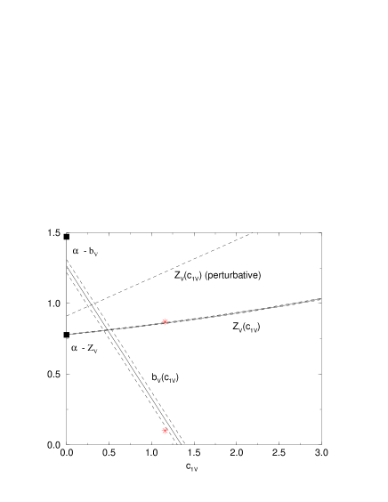
Figure 1: Results for $Z_{V}$ and $b_{V}$ against $c_{1V}$ for $\beta=6.0$. The error bars are given by bands of dotted lines. Also plotted is the one-loop perturbative result for $Z_{V}$ and the Alpha Collaboration results.

The Alpha Collaboration has non-perturbatively found $Z_{V}(c_{1V}=0)$ and $b_{V}(c_{1V}=0)$, [4]. We see from the figure that there is very good agreement between the different determinations for $Z_{V}(c_{1V}=0)$ and although for $b_{V}(c_{1V}=0)$ there is some discrepancy we note that this is not unexpected as $b_{V}$ has $O(a)$ effects. Also shown are two points (stars) from a method described in [5]. Again there is good agreement (this time at a non-zero value of $c_{1V}$).

For the axial current, again the Alpha Collaboration has non-perturbatively found $Z_{A}(c_{1A}=0)$, [4]. This is sufficient for us as we are only interested in the results in the chiral limit. Performing these extrapolations for $\beta=6.0$, $6.2$ gives the scaling plot, Fig. 2.

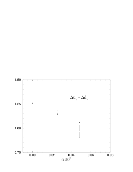
Figure 2: A scaling plot of $\Delta u_{v}-\Delta d_{v}\equiv g_{A}$ against $a^{2}$, using the string tension to set the scale. The Symanzik improved data at $\beta=6.0$, $6.2$ is shown with filled squares, the Wilson data, open square, is at $\beta=6.0$. The physical value of $g_{A}=1.26$.

To attempt a comparison with Wilson data, we have also plotted the result at $\beta=6.0$, [2] using the non-perturbative $Z_{A}$ as found in [5] of $0.78$. This is close to the value ($0.75$) given from linearly interpolating the non-perturbative Ward Identity results in [7] to $\beta=6.0$, which would indicate that $O(a)$ effects between these two methods are small. In Fig. 2 we expect to have to make a linear extrapolation in $a^{2}$ for the improved case.

For $\langle x\rangle$ there is no non-perturbative determination of the renormalisation constants yet available. First order perturbation theory gives, however, numbers rather close to $1$, [6], and indeed using tadpole improved ($TI$) perturbation theory, we see that with one derivative operators the (large) tadpole terms cancel. This might indicate that perturbation theory is reasonably correct. From the definition of the improved operator we see that we have parameters $b_{0}$, $c_{1}$, $c_{2}$. To remove $O(a)$ effects completely we must only have a residual one parameter degree of freedom (from the $EOM$), so that, eg, $c_{2}\equiv c_{2}(c_{1})$ and $b_{0}\equiv b_{0}(c_{1})$. These functions are unknown at present. At tree level $c_{2}=c_{1}$, $b_{0}=1-c_{1}$, which we shall use here. In Fig. 3

Figure 3: A comparison between first order perturbation theory and $TI$ perturbation theory, using the boosted coupling $\alpha^{\overline{MS}}(\mu a)$ given in table $I$ of [8]. Also used in the perturbative coefficient is $\tilde{c}_{sw}=c_{sw}(g^{2})u_{0}^{3}$, ($u_{0}^{4}=\langle\mbox{\small$\frac{1}{3}$}\mbox{tr}U_{plaq}\rangle$).

we compare one loop perturbative results, and $TI$ results for $\langle x\rangle^{(u)}$ in the chiral limit. We know that upon using the true coefficients then the result must be independent of $c_{1}$. $TI$ appears to achieve this somewhat better than $1$-loop perturbation expansion, so we shall use this in our scaling plot shown in Fig. 4.

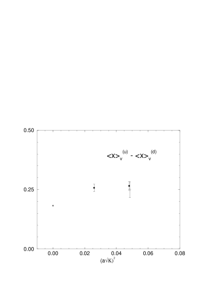
Figure 4: Scaling plot of non-singlet $\langle x\rangle_{v}^{(u)}-\langle x\rangle_{v}^{(d)}$ against $a^{2}$, using $c_{1}=0$. Same notation as in Fig. 2.

This operator has an anomalous dimension, so we must scale the results to the same $\mu$; this has been performed with the scaling formula $\langle x\rangle|_{\mu}=(\alpha_{\overline{MS}}(\mu)/\alpha_{\overline{MS}}(\mu_{0}))^{32/99}\langle x\rangle|_{\mu_{0}}$. Scaling the $\beta=6.2$ result to $\beta=6.0$ where $\mu\sim 1.95(\mbox{GeV})^{-1}$ gives a $4\%$ increase. We compare with the phenomenological value, [9]. Our results seem rather constant (in $a^{2}$), suggesting that even in the continuum limit the lattice value is too high. We can only speculate on the discrepancy: most likely this is due to a lattice problem – quenching, chiral extrapolation, $Z$ not accurately enough known or perhaps there is a phenomenological problem – the fits are made from low $\mu^{2}$ so there might be higher twist contributions, [10].

References

[1] P. Stephenson, D. Pleiter, this conference.
[2] M. Göckeler, R. Horsley, E.-M. Ilgenfritz,
H. Perlt, P. Rakow, G. Schierholz and A. Schiller,
Phys. Rev. D53 (1996) 2317, hep-lat/9508004.
[3]
B. Sheikholeslami and R. Wohlert,
Nucl. Phys. B259 (1985) 572.
[4] M. Lüscher et al,
Nucl. Phys. B491 (1997) 323, hep-lat/9609035;
ibid B491 (1997) 344, hep-lat/9611015.
[5] P. Rakow and H. Oelrich, this conference.
[6] S. Capitani, this conference.
[7] S. Aoki et al,
Nucl. Phys. B(Proc. Suppl.) 53 (1997) 2109,
hep-lat/9608144.
[8] G. P. Lepage and P. B. Mackenzie,
Phys. Rev. D48 (1993) 2250, hep-lat/9209022.
[9] A. D. Martin et al,
Phys. Lett. B354 (1995) 155, hep-ph/9502336.