B spectroscopy using all-to-all propagators

Abstract

We measure the ground and excited states for B mesons in the static limit using maximally variance reduced estimators for light quark propagators. Because of the large number of propagators we are able to measure accurately also orbitally excited $P,D$ and $F$ states. We also present some results for $\Lambda_{b}$.

1 INTRODUCTION

Usually one calculates the light quark propagators needed for hadronic observables in lattice QCD by exact inversion from one source. It is necessary to iterate almost to machine precision to avoid introducing bias. This is clearly wasteful, as the variation from one gauge to another can be large. The situation is even more severe for static quarks, when one gets only one number per inversion.

Stochastic estimators for an inverse of a positive definite matrix $M$ are easily obtained from

$$M_{ij}^{-1}=\left<\phi_{i}^{*}\phi_{j}\right>={1\over Z}\int d\phi e^{-{1\over 2}\phi^{*}M\phi}.$$ (1)

Unfortunately the Wilson-Dirac fermion matrix $Q$ is positive definite only for extremely small values of hopping parameter $K$. This problem can be solved by taking $M=Q^{\dagger}Q$, and calculating the propagator from

$$G_{ij}=Q^{-1}_{ji}=\left<(Q_{ik}\phi_{k})^{*}\phi_{j}\right>.$$ (2)

This stochastic estimate can be used to calculate any hadronic observable, but because one is usually interested in exponential decay of correlators at large $T$ values, the variance coming from stochastic inversion will kill the signal rather quickly. Therefore one would prefer to use improved operators; this can be achieved using variance reduction.

2 MAXIMAL VARIANCE REDUCTION

One suggestion is to use local multi-hit variance reduction for $\phi$ fields [1]; this is very easy to implement and provides significant error reduction. However, as the action is quadratic in $\phi$ one should be able to implement a method that takes into account not only the nearest neighbours of $\phi$, but all fields inside some given region $P$.

If the scalar fields inside region $P$ and on the boundary of $P$ are called $\phi$ and $s$ respectively, one can obtain maximally variance reduced estimate for $\phi(x)$ by

$$v_{i} = {1\over Z}\int D\phi\,\,\phi_{i}\times$$ (3)

$$\exp(-{1\over 2}\phi_{j}^{*}\hat{M}_{jk}\phi_{k}+\phi_{j}^{*}\bar{M}_{jk}s_{k}+h.c.)$$

where we have also distinguished the elements of M connecting $\phi_{i}$ to only fields inside $P$ ($\hat{M}$) and those connecting $\phi_{i}$ to the boundary ($\bar{M}$). The integral (3) is Gaussian and one obtains easily

$$v_{i}=-\hat{M}_{ij}^{-1}\bar{M}_{jk}s_{k}.$$ (4)

We will call $v_{i}$ the maximally variance reduced stochastic estimator for $\phi_{i}$.

To form propagators, we need a product of two $\phi$ fields. This means that it is not sufficient to improve only one field within $P$, but one must choose two disjoint regions $P$ and $R$ and solve for two variance reduced fields $v$ and $w$ respectively. Then one can apply (2) to obtain

$$G_{ij}=\left<(Q_{ik}v_{k})^{*}w_{j}\right>$$ (5)

with no bias.

3 B MESONS AND $\Lambda_{b}$

Consider mesons containing one infinitely heavy quark $Q$ and one light quark $q$. Such a system is obtained in leading order heavy quark effective theory HQET [2] for the B meson. This system is particularly suitable for stochastic inversion as usually one is only able to obtain one number per inversion.

The expectation value one has to calculate contains simply one light propagator and the product of gauge links $U$. This is easily obtained from equation (5). In addition one can use smearing (or fuzzing) to create different sources; in particular it is possible to construct operators corresponding to orbitally excited states by using techniques from [3].

It is also possible to construct observables with more than one light quark. $\Lambda_{b}$ in leading order HQET contains one infinitely heavy quark and two light quarks. This is also easily obtained from stochastically improved fields $v,w$ but a little care is needed. One way to grasp the subtlety is to imagine that there are two quarks with different flavours. Then one has to split the sum over samples $\alpha=1\ldots N$ into subsets for each flavour. If these subset are independent, one obtains propagators of each flavour with no bias. In practice if the stochastic estimators $\phi^{\alpha}$ are independent of $\alpha$, one can calculate the required propagators from

$$G_{ij}^{\alpha}G_{i^{\prime}j^{\prime}}^{\beta}=\sum_{\alpha\neq\beta}(Q_{ik}v_{k}^{\alpha})^{*}(Q_{i^{\prime}k^{\prime}}v_{k^{\prime}}^{\beta})^{*}w_{j}^{\alpha}w_{j^{\prime}}^{\beta}.$$ (6)

The $\Lambda_{b}$ correlator is then easily constructed by multiplying two light quark propagators from equation (6) by the gauge links corresponding to a heavy quark propagator.

4 RESULTS

Figure 1: Effective mass plot for $S$-wave with hopping parameter $K_{1}=0.14077$ corresponding to roughly strange quark mass.

We have performed simulations with tadpole improved quenched clover action ($c_{SW}=1.57$), with $\beta=5.7$. The lattice size we use is rather small, $12^{3}\times 24$. We work with two different hopping parameters $K_{1}=0.14077$ and $K_{2}=0.13843$. The same values of hopping parameters are used also in [4], and we use those results also to set our scale. The values $K_{1}$ and $K_{2}$ correspond to the strange quark and twice the strange light quark masses respectively.

We use 20 gauge configurations, and in each of them we calculate 24 stochastic samples for each hopping parameter. The stochastic update consisted of 5 overrelaxation steps followed by one heat bath. Measurements were taken after every 25 combined OR/HB sweeps and the system was thermalised for 50 heat bath sweeps before the first measurement.

The choice of the regions $P$ and $R$ is rather arbitrary; we chose to divide the lattice by time planes at $T=1$ and $T=9$. We used two different fuzzing levels for all operators.

A typical effective mass plot can be seen in Figure 1, where we have plotted the effective mass of the $L=0$ (S) state together with factorising fit.

Our full results can be seem from Figure 2, where we have plotted the mass splittings between excited states and ground state in units of $r_{0}$. Also included is the mass splitting of $\Lambda_{b}$ and the ground state of $B$. Note that the ordering of P-waves we observed before [5] has now changed.

These results should be compared to results obtained using usual inversion techniques. In Figure 3 we have plotted results several other groups [6, 7, 8] have obtained using much more computing resources. Our results are clearly consistent with theirs. However, we have much smaller errorbars and are able to obtain reliably several excited states, which is not generally true for the earlier work in the static limit. One should also note that our results are compatible with results obtained from non-relativistic QCD [9].

Because we have not yet estimated systematic errors arising from finite lattice size and spacing, we chose not to extrapolate our results to the chiral limit.

Figure 2: The spectrum of B meson containing one light (with mass proportional to pseudoscalar mass $m_{P}^{2}$) and one infinitely heavy quark. Also included are our results for $\Lambda_{b}$.

5 CONCLUSIONS

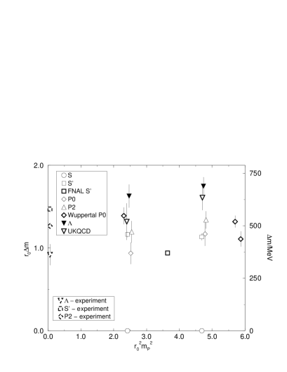
Figure 3: Comparison with earlier results. FNAL group [6] has only estimated the excited S-wave with no error. UKQCD results for $\Lambda_{b}$ are from [7], Wuppertal results for P0 from [8]. The experimental values [10, 11] are for real $B$ meson and $\Lambda_{b}$, so one would expect to see some difference from leading order HQET.

We have shown that stochastic estimators for light quark propagators are extremely useful in heavy quark effective theory, where the usual method of calculating light quark propagators is extremely wasteful. We have obtained reliable signals for the first time for excited states in the static limit, and show that even states with $L=3$ (F-waves) can be obtained.

It is obvious that our method can be used successfully not only for spectroscopy but also for matrix elements. The ability to obtain reliable information on excited states is valuable when one is trying to extract the heavy-light decay constant $f_{B}$.

References

- [1] G. de Divitiis et al. Phys. Let., B382 (1996) 393.
- [2] See, for example, M. Neubert, Phys. Rept. 245 (1994) 259, and references therein.
- [3] UKQCD Collaboration, P. Lacock et al., Phys. Rev. D54 (1996) 6997.
- [4] UKQCD Collaboration, H.P. Shanahan et al. Phys.Rev. D55 (1997) 1548
- [5] C. Michael and J. Peisa. hep-lat/9705013.
- [6] A. Duncan et al. Phys. Rev. D51 (1995) 5101.
- [7] UKQCD Collaboration, A. Ewing et al. Phys. Rev. D54 (1996) 3526.
- [8] C. Alexandrou et al. Nucl. Phys. B414 (1994) 815.
- [9] For a review, see plenary talk by Arifa Ali Khan, these proceedings.
- [10] C. Weiser. Proceedings of the 28th International Conference on High Energy Physics, Warsaw 1996, p. 531. Ed. I. Adjuk and A. Wroblewski, World Scientific 1996.
- [11] R.M. Barnett et al., Phys. Rev. D54 1, (1996)