High-$T$ QCD and dimensional reduction: measuring the Debye mass

Abstract

We study the high-temperature phase of SU(2) and SU(3) QCD using lattice simulations of an effective 3-dimensional SU($N$) + adjoint Higgs -theory, obtained through dimensional reduction. We investigate the phase diagram of the 3D theory, and find that the high-$T$ QCD phase corresponds to the metastable symmetric phase of the 3D theory. We measure the Debye screening mass $m_{D}$ with gauge invariant operators; in particular we determine the ${\cal O}(g^{2})$ and ${\cal O}(g^{3})$ corrections to $m_{D}$. The corrections are seen to be large, modifying the standard power-counting hierarchy in high temperature QCD.

The Debye mass (inverse screening length of color electric fields) characterizes the coherent static interactions in QCD plasma, and its numerical value is essential for phenomenological discussion of the physics of the QCD plasma. For SU($N$) QCD, $N=2,3$, with $N_{f}$ massless quarks, the Debye mass can be expanded at high temperatures in a power series in the coupling $g$:

$$m_{D} = m_{D}^{\mbox{\scriptsize LO}}+{Ng^{2}T\over 4\pi}\ln{m_{D}^{\mbox{\scriptsize LO}}\over g^{2}T}$$ (1)

$$+ c_{N}g^{2}T+d_{N,N_{f}}g^{3}T+{\cal O}(g^{4}T),$$

where the leading order perturbative result is $m_{D}^{\mbox{\scriptsize LO}}=(N/3+N_{f}/6)^{1/2}gT$. The logarithmic part of the ${\cal O}(g^{2})$ correction can be extracted perturbatively [1], but $c_{N}$ and the higher order corrections are non-perturbative. Our aim is to evaluate numerically the coefficients $c_{N}$ and $d_{N,N_{f}}$. A detailed discussion of the results can be found in [2, 3].

An effective 3D action, obtained through dimensional reduction  [4, 5, 6], is a powerful tool for studying high-$T$ QCD. The effective action can be derived perturbatively without the infrared problems associated with the standard high-$T$ perturbative analysis. It retains the essential infrared physics of the original theory, and since it is bosonic even for $N_{f}>0$, it can be studied economically with lattice Monte Carlo simulations. Recently it has been very successfully applied to the Electroweak phase transition [7].

The effective action is derived with the Green’s function matching technique [5, 6]:

$$L_{\mbox{\scriptsize eff}} = {\mbox{${\frac{1}{4}}$}}F_{ij}^{a}F_{ij}^{a}+{\rm Tr\,}[D_{i},A_{0}][D_{i},A_{0}]$$ (2)

$$+ m_{3}^{2}{\rm Tr\,}A_{0}^{2}+\lambda_{A}({\rm Tr\,}A_{0}^{2})^{2}\,.$$

$A_{0}$ is a remnant of the temporal gauge fields and belongs to the adjoint representation of SU($N$). The Lagrangian (2) gives the Green’s functions to a relative accuracy ${\cal O}(g^{4})$ [5], sufficient for the accuracy of the expansion in eq. (1).

For $N_{f}=0$, the 3D couplings $g_{3}^{2}$, $m_{3}^{2}$ and $\lambda_{A}$ are related to the temperature $T$ (and the 4D gauge coupling $g^{2}(\mu)$, which is evaluated at the optimized scale [2] $\mu\approx 2\pi T$) by

$$g_{3}^{2}=g^{2}T = {\frac{24\pi^{2}T}{22\log(6.742T/\Lambda_{\overline{\rm MS}})}}$$ (3)

$$x\equiv{\frac{\lambda_{A}}{g_{3}^{2}}} = {\frac{6+N}{11N}}{\frac{1}{\log(5.371T/\Lambda_{\overline{\rm MS}})}}$$ (4)

$$y\equiv\frac{m_{3}^{2}}{g_{3}^{4}} = {\frac{2}{9\pi^{2}x}}+{\frac{4}{16\pi^{2}}}+{\cal O}(x){\hskip 14.22636pt}\mbox{SU(2)}$$ (5)

$$= {\frac{3}{8\pi^{2}x}}+{\frac{9}{16\pi^{2}}}+{\cal O}(x){\hskip 14.22636pt}\mbox{SU(3)}$$ (6)

The dynamics of the 3D theory is fully characterized by the dimensionless ratios $x$ and $y$ above and the dimensionful gauge coupling $g_{3}^{2}$. The presence of fermions only modifies the numerical factors in eqs. (3–6).

Due to the superrenormalizability of the 3D action the continuum$\leftrightarrow$lattice relations of the couplings become very transparent (for a detailed discussion, see [2, 8]). In particular, the lattice gauge coupling $\beta_{G}$ is related to the continuum gauge coupling $g_{3}^{2}$ and the lattice spacing $a$ by $\beta_{G}=2N/(g_{3}^{2}\,a)$.

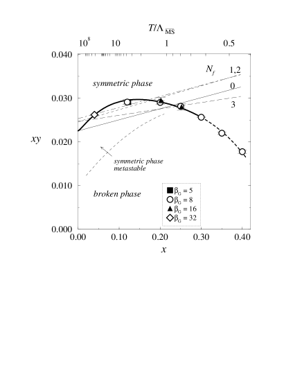
Figure 1: The phase diagram of the 3D SU(2) + adjoint Higgs theory. The plot symbols show the location of the transition given by the simulations (extrapolated to $V\rightarrow\infty$), and the $y=y_{c}(x)$ curve is a 4th order polynomial interpolation of the data. Dashed line indicates where the transition becomes a cross-over. The straight lines are the ‘dimensional reduction lines’ $y_{\rm dr}(x)$ for the number of fermion flavors indicated.

The phase diagram of the SU(2) + adjoint Higgs theory is shown in Fig. 1 (for convenience, plotted in the ($x,xy$)-plane). For SU(3) the diagram is qualitatively similar. At small $x$, the transition is very strongly first order, but becomes rapidly weaker when $x$ increases. At $x\approx 0.32$ there is a critical point, after which only a cross-over remains. The $N_{f}=0$ $y_{\rm dr}(x)$ -line is given in eq. (5). The 3D theory is well defined on the entire $(x,y)$-plane, but only along $y_{\rm dr}(x)$ does the 3D theory describe the physics of the 4D SU(2) gauge theory. Along this line $x$ is related to the temperature as shown on the top axis of the plot (for SU(2), $\Lambda_{\overline{\rm MS}}\approx 1.2T_{c}$).

In the physically relevant region $T\gg T_{c}\sim\Lambda_{\overline{\rm MS}}$ the $y_{\rm dr}$ line is in the broken phase . However, the 3D theory cannot describe 4D high-$T$ physics in the broken phase, since the perturbative 4D$\leftrightarrow$3D connection is not valid there [2]. Thus the symmetric phase is the physical one. Due to the strong 1st order nature of the transition at small $x$, the symmetric phase is strongly metastable  (shown with the dashed line in Fig. 1). If initially prepared to be in the symmetric phase, the system remains there for the duration of any realistic Monte Carlo simulation.

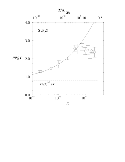
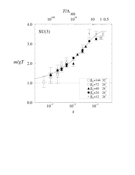
Figure 2: The Debye mass for SU(2) (top) and SU(3) (bottom), as functions of $x$ (top scales show $T/\Lambda_{\overline{\rm MS}}$ through eq. (4)). The dashed line indicates the leading order $m_{D}^{\mbox{\scriptsize LO}}$, and the continuous line the 2-parameter fit to eq. (1) with the parameters as in eq. (8).

The Debye mass can be defined as the mass of the lightest 3d state odd under the reflection $A_{0}\rightarrow-A_{0}$ [9]. The lowest-dimensional gauge invariant operator fulfilling this is

$$h_{i}=\epsilon_{ijk}{\rm Tr\,}A_{0}F_{jk}\,.$$ (7)

To enhance the signal, we measure the correlation function $\langle h_{i}(0)h_{i}(z)\rangle$ using several recursive blocking levels [2]. We perform the measurements along the metastable $y_{\rm dr}(x)$ -lines, eqs. (5,6). The results are shown in Fig. 2, in units of 4D $gT$ ($=g_{3}^{2}\sqrt{3y/N}$ in 3D units). The Monte Carlo runs are performed with several lattice spacings $a$ ($\beta_{G}$). The top scales in Fig. 2 show the physical temperature $T/\Lambda_{\overline{\rm MS}}$ along $y_{\rm dr}(x)$ -lines. Note that the highest temperatures are larger than $10^{100}\times\Lambda_{\overline{\rm MS}}\sim 10^{100}\times T_{c}$.

We fit the data to the 2-parameter ansatz in eq. (1). At small $x$ (large $y$), the quality of the fits is very good. We use only data in the range $x<0.08$, so that the horizontal plateaus at large $x$ are excluded from the fits. The results of the fits are [3]

$$\begin{array}[]{cll}\mbox{SU(2):}&c_{2}=1.58(20)&b_{2}=-0.03(25)\\ \mbox{SU(3):}&c_{3}=2.46(15)&b_{3}=-0.49(15)\,,\end{array}$$ (8)

where $b_{N}=d_{N,N_{f}}\sqrt{N/3+N_{f}/6}$. For $N=2$ we can only verify that $d_{2,N_{f}}$ is close to zero. Note that writing $c_{N}=N\tilde{c}_{N}$, one has $\tilde{c}_{N}=0.79\pm 0.10$ ($N=2$), $0.82\pm 0.05$ ($N=3$).

The leading contribution to $m_{D}$ is dominant only at extremely large $T$ – indeed, for SU(3) the leading term is larger than the ${\cal O}(g^{2})$ correction for $T/\Lambda_{\overline{\rm MS}}\mathop{\raise 1.29167pt\hbox{$>$\kern-7.5pt\raise-4.73611pt\hbox{$\sim$}}}10^{19}$, implying that the leading term only dominates when QCD anyway merges into a unified theory. For temperatures around $T\sim 1000\Lambda_{\overline{\rm MS}}$ the non-perturbative $m_{D}$ is already about $3\times m_{D}^{\rm LO}$. For a detailed discussions, we refer to [3]. Large corrections to leading order $m_{D}$ have also been observed in 4D $N_{f}=0$ SU(2) simulations, using gluon mass measurements in the Landau gauge [10]. It remains to be seen whether this modification of the standard picture of high-temperature gauge theories has applications in the cosmological discussion of the quark-hadron phase transition or in the phenomenology of heavy ion collisions.

References

- [1] A.K. Rebhan, Phys. Rev. D 48, R3967 (1993); Nucl. Phys. B 430, 319 (1994).
- [2] K. Kajantie, M. Laine, K. Rummukainen and M. Shaposhnikov, Nucl. Phys. B, in press [hep-ph/9704416]; K. Rummukainen, hep-lat/9707034.
- [3] K. Kajantie, M. Laine, J. Peisa, A. Rajantie, K. Rummukainen and M. Shaposhnikov, Phys. Rev. Lett, in press [hep-ph/9708207].
- [4] P. Ginsparg, Nucl. Phys. B 170, 388 (1980); T. Appelquist and R. Pisarski, Phys. Rev. D 23, 2305 (1981); S. Nadkarni, Phys. Rev. D 27, 917 (1983).
- [5] K. Kajantie, K. Rummukainen and M. Shaposhnikov, Nucl. Phys. B 407, 356 (1993); K. Kajantie, M. Laine, K. Rummukainen and M. Shaposhnikov, Nucl. Phys. B 458, 90 (1996).
- [6] E. Braaten and A. Nieto, Phys. Rev. D 51, 6990 (1995); Phys. Rev. D 53, 3421 (1996).
- [7] For a review, see K. Rummukainen, Nucl. Phys. B (Proc. Suppl.) 53, 30 (1997).
- [8] M. Laine and A. Rajantie, HD-THEP-97-16 [hep-lat/9705003].
- [9] P. Arnold and L.G. Yaffe, Phys. Rev. D 52, 7208 (1995).
- [10] U. Heller, F. Karsch and J. Rank, these proceedings; hep-lat/9708009.