FSU–SCRI–97–94 hep–lat/9708024
The Local Hybrid Monte Carlo Algorithm for
Free Field Theory:
Reexamining Overrelaxation

Abstract

We analyze the autocorrelations for the Local Hybrid Monte Carlo algorithm [1] in the context of free field theory. In this case this is just Adler’s overrelaxation algorithm [2]. We consider the algorithm with even/odd, lexicographic, and random updates, and show that its efficiency depends crucially on this ordering of sites when optimized for a given class of operators. In particular, we show that, contrary to previous expectations, it is possible to eliminate critical slowing down (${z_{\mbox{\tiny int}}}=0$) for a class of interesting observables, including the magnetic susceptibility: this can be done with lexicographic updates but is not possible with even/odd (${z_{\mbox{\tiny int}}}=1$) or random (${z_{\mbox{\tiny int}}}=2$) updates. We are considering the dynamical critical exponent ${z_{\mbox{\tiny int}}}$ for integrated autocorrelations rather than for the exponential autocorrelation time; this is reasonable because it is the integrated autocorrelation which determines the cost of a Monte Carlo computation.

1 Introduction

Stochastic overrelaxation, and especially its variant usually referred to as “hybrid overrelaxation,” is generally considered to be the most efficient algorithm for generating lattice configurations in pure gauge theory. As such it is also frequently used for the purposes of quenched simulations, although at the currently studied (small) correlation lengths the relative improvement over the standard Metropolis or heatbath local algorithms is a priori rather modest.

The idea of generalizing overrelaxation methods to the stochastic case is due to Adler [2], who proposed an algorithm for multiquadratic actions such as free field theory (see also [3]). The initial expectations of improved performance were confirmed by studying the dynamical critical behaviour of the algorithm in this context analytically [4, 5, 6, 7]. The main result of these studies was that the algorithm can be tuned to achieve the dynamical critical exponent ${z_{\mbox{\tiny exp}}}=1$ as compared to the generic value ${z_{\mbox{\tiny exp}}}=2$ for the standard local Metropolis or heatbath algorithms. Some additional theoretical insights were also obtained in references [8, 9].

Several extensions of the algorithm to interacting field theories and subsequent partial modifications were introduced by various authors, including [5, 10, 11, 12, 13, 14]. These algorithms were studied in more detail in several numerical works such as [15, 16, 17, 18]. While these almost invariably claim useful improvement, the truly systematic study (such that could make reasonable conclusions about dynamical critical exponents) is still missing.

The purpose of this paper is to analyze the free field behaviour of overrelaxation further. Apart from our original aim of evaluating certain autocorrelations, we obtained some interesting conceptual insights which we feel are worth communicating. It has become clear over the years that the performance of Monte Carlo algorithm should be assessed with respect to a given operator $\Omega$ (or set of operators): in particular, the most relevant characteristic then is the dynamical critical exponent $z_{\Omega}$, corresponding to the integrated autocorrelation for that quantity. While the dynamical critical exponent for the exponential autocorrelation time (which we denoted by ${z_{\mbox{\tiny exp}}}$ in previous paragraphs) usually gives us an upper bound, it often happens that $z_{\Omega}<{z_{\mbox{\tiny exp}}}$ for most observables.

If we have a situation where for operators of interest, $z_{\Omega}$ can be made smaller than ${z_{\mbox{\tiny exp}}}$, then the latter is somewhat irrelevant for the task at hand. In lattice field theory we actually have a specific group of operators we want to speed up, namely the ones for which the low energy (momentum) states are most important, because these operators are relevant for the continuum limit. We should thus attempt to optimize the overrelaxation algorithm for these quantities, rather than minimize ${z_{\mbox{\tiny exp}}}$. It has been implicitly assumed in previous studies that zero momentum operators (such as the magnetic susceptibility) actually saturate the ${z_{\mbox{\tiny exp}}}$-bound and so the above distinction is just a wishful thinking. Our main point in this paper is that while this is true for even/odd updates, where the dynamics of overrelaxation intrinsically couples the low and high frequency modes, it is not true for lexicographic updates, where the modes decouple at large volumes. In fact in the latter case we can tune the overrelaxation algorithm such that critical slowing down is completely eliminated for quantities that depend only on the zero momentum mode. We emphasize that this is a different tuning than the one leading to ${z_{\mbox{\tiny exp}}}=1$; in fact, with this tuning ${z_{\mbox{\tiny exp}}}=2$. However, in this case the ${z_{\mbox{\tiny exp}}}$-bound is actually saturated by high frequency quantities most of which we are not interested in.

In the light of the above discussion, the “conventional wisdom” about the inability of local algorithms to perform better than ${z_{\mbox{\tiny exp}}}\approx 1$ (see for example [9]) can be rather misleading. While the statement as such might be true (but has not been proved even for free field theory), it does not tell us much about how the local algorithm will perform in the specific case of interest.

The second point we want to make concerns the introduction of the additional noise in the overrelaxation update. In particular we attempted the same optimization for a scheme in which the updated site is chosen at random from a uniform distribution. It turns out that in this case it is impossible to tune the overrelaxation parameter to reduce the critical slowing down for zero momentum quantities; in fact we cannot do better than $z_{\Omega}=2$ for these operators. This means that overrelaxation can easily lose its magic if we introduce extra noise in the procedure.

In [1] it was shown that the overrelaxation algorithm for free field theory is a special case of the class of Hybrid Molecular Dynamics algorithms where the fields are updated one site at a time using an analytic solution of the equations of motion. This rather suprising and elegant connection is especially intriguing in the light of the fact that, as shown in [14], a corresponding algorithm can be found for gauge theories. Here we adopt this point of view and will frequently refer to free field overrelaxation as Local Hybrid Monte Carlo (LHMC).

We start in section 2 by formulating the LHMC algorithm and developing the techniques to calculate the integrated autocorrelations for typical zero momentum quantities, namely magnetization and susceptibility. In section 3 we analyze the performance of LHMC with even/odd, lexicographic, and random updates. We also give a proof that the integrated autocorrelation for the magnetic susceptibility vanishes at large volume with optimally tuned overrelaxation parameter when using the modified lexicographic update. In Appendix A we give an explicit asymptotic calculation of the update matrix for the lexicographic scheme, and in Appendix B we develop a formalism for bounding the finite volume corrections using methods of functional analysis.

2 Local Hybrid Monte Carlo for Free Field Theory

2.1 Analytic Solution

We wish to consider a real scalar free field theory described by a functional integral with the usual action

$$S[\phi]\equiv{\mathchoice{\textstyle{1\over 2}}{\scriptstyle{1\over 2}}{\scriptscriptstyle{1\over 2}}{1/2}}\sum_{x\in{\twelvebb Z}_{L}^{d}}\{-\phi_{x}\Delta\phi_{x}+m^{2}\phi_{x}^{2}\},$$

and a flat (Lebesgue) measure for the $\phi$ field. The lattice Laplacian operator is defined as

$$\Delta\phi_{x}\equiv\sum_{\mu=1}^{d}(\phi_{x+\hat{\mu}}-2\phi_{x}+\phi_{x-\hat{\mu}}),$$

where $\hat{\mu}$ is a unit vector in the $\mu$ direction. Since the theory is free it can be diagonalized using the Fourier transformed fields

$$\phi_{x}\equiv L^{-d/2}\sum_{p\in{\twelvebb Z}_{L}^{d}}{\tilde{\phi}}_{p}e^{2\pi ip\cdot x/L},$$

where ${\tilde{\phi}}_{p}^{*}={\tilde{\phi}}_{-p}$ since $\phi_{x}\in{\twelvebb R}$. The action simplifies to

$$S[{\tilde{\phi}}]={\mathchoice{\textstyle{1\over 2}}{\scriptstyle{1\over 2}}{\scriptscriptstyle{1\over 2}}{1/2}}\sum_{p\in{\twelvebb Z}_{L}^{d}}f_{p}^{2}|{\tilde{\phi}}_{p}|^{2}$$ (1)

with

$$f_{p}^{2}\equiv m^{2}+2d-2\sum_{\mu=1}^{d}\cos{2\pi p_{\mu}\over L}\;.$$

In particular we note that the lowest and highest frequencies of the system are $f_{(0,\ldots,0)}^{2}=m^{2}$ and $f_{({\mathchoice{\textstyle{1\over 2}}{\scriptstyle{1\over 2}}{\scriptscriptstyle{1\over 2}}{1/2}}L,\ldots,{\mathchoice{\textstyle{1\over 2}}{\scriptstyle{1\over 2}}{\scriptscriptstyle{1\over 2}}{1/2}}L)}^{2}=m^{2}+4d$.

2.2 Local Hybrid Monte Carlo Updates

Consider the dependence of the action $S$ upon one degree of freedom only, $S(\phi_{x})={\mathchoice{\textstyle{1\over 2}}{\scriptstyle{1\over 2}}{\scriptscriptstyle{1\over 2}}{1/2}}\omega^{2}\phi_{x}^{2}-{\cal F}_{x}\phi_{x}+\mbox{constant}$, where here $\omega^{2}\equiv m^{2}+2d$ and ${\cal F}_{x}\equiv\sum_{\mu=1}^{d}(\phi_{x+\hat{\mu}}+\phi_{x-\hat{\mu}})$. Introducing the fictitious Hamiltonian $H(\phi_{x},\pi_{x})\equiv{\mathchoice{\textstyle{1\over 2}}{\scriptstyle{1\over 2}}{\scriptscriptstyle{1\over 2}}{1/2}}\pi_{x}^{2}+S(\phi_{x})$ we have

$$H={\mathchoice{\textstyle{1\over 2}}{\scriptstyle{1\over 2}}{\scriptscriptstyle{1\over 2}}{1/2}}\left[\pi_{x}^{2}+\omega^{2}\left(\phi_{x}-{{\cal F}_{x}\over\omega^{2}}\right)^{2}\right]+\mbox{constant},$$

and the solution of the corresponding equations of motion is

$$\phi_{x}(t)-{{\cal F}_{x}\over\omega^{2}}=\left(\phi_{x}(0)-{{\cal F}_{x}\over\omega^{2}}\right)\cos\omega t+{\pi_{x}(0)\over\omega}\sin\omega t,$$

or

$$\phi^{\prime}_{x}=(1-\zeta)\phi_{x}+{\sqrt{\zeta(2-\zeta)}\over\omega}\pi_{x}+{{\cal F}_{x}\over\omega^{2}}\zeta$$ (2)

in terms of the overrelaxation parameter $\zeta\equiv 1-\cos\omega t$.

Assembling the field variables and their conjugate fictitious momenta into the vectors

$$\phi\equiv\left(\begin{array}[]{c}\phi_{x_{1}}\\ \phi_{x_{2}}\\ \vdots\\ \phi_{x_{L^{d}}}\end{array}\right)\qquad\mbox{and}\qquad\pi\equiv\left(\begin{array}[]{c}\pi_{x_{1}}\\ \pi_{x_{2}}\\ \vdots\\ \pi_{x_{L^{d}}}\end{array}\right)$$ (3)

we can write the elementary local update (2) in the form

$$\phi\mapsto M_{x}\phi+P_{x}\pi;$$ (4)

here $M_{x}$ and $P_{x}$ are $L^{d}\times L^{d}$ matrices, and the subscript refers to the site being updated. More explicitly, we have

$$(M_{z})_{x,y} = \delta_{x,y}+\delta_{x,z}\Bigl{[}-\zeta\delta_{x,y}+{\zeta\over\omega^{2}}\sum_{\mu=1}^{d}(\delta_{x+\hat{\mu},y}+\delta_{x-\hat{\mu},y})\Bigr{]},$$ (5)

$$(P_{z})_{x,y} = \delta_{x,y}\delta_{x,z}{\sqrt{\zeta(2-\zeta)}\over\omega}.$$

Definition (3) implicitly assumes that we have ordered the field variables in a certain way. Sweeping through the lattice in this order, the complete update is given by

$$\phi \mapsto M_{x_{1}}\phi+P_{x_{1}}\pi\mapsto(M_{x_{2}}M_{x_{1}})\phi+(M_{x_{2}}P_{x_{1}}+P_{x_{2}})\pi$$

$$\mapsto\cdots\mapsto\left(\prod_{j=1}^{L^{d}}M_{x_{j}}\right)\phi+\left[\sum_{i=1}^{L^{d}}\left(\prod_{j=i+1}^{L^{d}}M_{x_{j}}\right)P_{x_{i}}\right]\pi\equiv M\phi+P\pi.$$ (6)

Note that the form of the matrices $M$ and $P$ depends upon the predetermined order in which we chose to sweep through the lattice. In fact, as we shall discuss, the efficiency of the algorithm (optimized for a given operator) can depend crucially on this order.

In addition to such fixed-order updates we will also analyze the algorithm in which the updated sites are chosen at random. The formulæ (4–6) carry over unchanged to this case except that the updated site becomes an uniformly distributed random variable over ${\twelvebb Z}_{L}^{d}$.

2.3 Cost of Measuring the Operators

If we are interested in measuring the expectation value of some operator $\Omega$, and $\bar{\Omega}$ is the average over a sequence of $T$ configurations generated by some Markov process, we expect

$$\bar{\Omega}=\langle\Omega\rangle\pm\sqrt{{2{\cal A}_{\Omega}+1\over T}\mathop{\rm Var}\Omega}.$$

Here $\mathop{\rm Var}\Omega=\langle\Omega^{2}\rangle-\langle\Omega\rangle^{2}$ is the intrinsic variance of $\Omega$, and ${\cal A}_{\Omega}$ is the integrated autocorrelation defined as

$${\cal A}_{\Omega}\equiv\sum_{t=1}^{\infty}{\Bigl{\langle}\Omega[\phi(t)]\Omega[\phi(0)]\Bigr{\rangle}-\Bigl{\langle}\Omega[\phi(t)]\Bigr{\rangle}\Bigl{\langle}\Omega[\phi(0)]\Bigr{\rangle}\over\bigl{\langle}\Omega^{2}\bigr{\rangle}-\bigl{\langle}\Omega\bigr{\rangle}^{2}}\equiv\sum_{t=1}^{\infty}{\cal C}^{c}_{\Omega}(t),$$

where ${\cal C}^{c}_{\Omega}$ is the connected autocorrelation function. The cost of measuring $\langle\Omega\rangle$ to a given accuracy depends upon ${\cal A}_{\Omega}$, and for local algorithms (such as LHMC) this is the only relevant characteristic which we need to compute in order to ascertain the performance of the algorithm. For a large system near criticality

$${\cal A}_{\Omega}\sim\xi^{z_{\Omega}}\qquad(1\ll\xi\ll L),$$

where $z_{\Omega}$ is the dynamical critical exponent, corresponding to quantity $\Omega$.

In this paper we are interested in studying the performance of LHMC when applied to measuring some interesting operators in the context of free field theory. To this end we shall mainly consider the magnetization ${\cal M}$ and magentization squared ${{\cal M}^{2}}$, where we define the magnetization as

$${\cal M}\equiv{1\over L^{d/2}}\sum_{x\in{\twelvebb Z}_{L}^{d}}\phi_{x}={\tilde{\phi}}_{0}.$$

The expectation values of powers of ${\cal M}$ are given by

$$\langle{\cal M}^{\alpha}\rangle=\langle{\tilde{\phi}}_{0}^{\alpha}\rangle={\int_{-\infty}^{\infty}d{\tilde{\phi}}_{0}\,e^{-{\mathchoice{\textstyle{1\over 2}}{\scriptstyle{1\over 2}}{\scriptscriptstyle{1\over 2}}{1/2}}f_{0}^{2}{\tilde{\phi}}_{0}^{2}}{\tilde{\phi}}_{0}^{\alpha}\over\int_{-\infty}^{\infty}d{\tilde{\phi}}_{0}\,e^{-{\mathchoice{\textstyle{1\over 2}}{\scriptstyle{1\over 2}}{\scriptscriptstyle{1\over 2}}{1/2}}f_{0}^{2}{\tilde{\phi}}_{0}^{2}}}=\left\{\begin{array}[]{ll}0&\mbox{if ${\mathchoice{\textstyle{1\over 2}}{\scriptstyle{1\over 2}}{\scriptscriptstyle{1\over 2}}{1/2}}\alpha\not\in{\twelvebb Z}$,}\\ {\Gamma\left({\alpha+1\over 2}\right)\over\Gamma({\mathchoice{\textstyle{1\over 2}}{\scriptstyle{1\over 2}}{\scriptscriptstyle{1\over 2}}{1/2}})}\left(2\over f_{0}^{2}\right)^{\alpha/2}&\mbox{if ${\mathchoice{\textstyle{1\over 2}}{\scriptstyle{1\over 2}}{\scriptscriptstyle{1\over 2}}{1/2}}\alpha\in{\twelvebb Z}$.}\end{array}\right.$$

In particular, $\langle{\cal M}\rangle=0$, $\langle{\cal M}^{2}\rangle={1\over m^{2}}$ and $\langle{\cal M}^{4}\rangle={3\over m^{4}}$. We thus expect that the measured values will satisfy $\overline{\cal M}=0\pm{1\over m}\sqrt{2{\cal A}_{\cal M}+1\over T}$, and $\overline{{{\cal M}^{2}}}={1\over m^{2}}\pm{\sqrt{2}\over m^{2}}\sqrt{2{\cal A}_{{\cal M}^{2}}+1\over T}$.

2.4 Autocorrelations

The general formalism for calculating the autocorrelations of any operator that is polynomial in the fields has been developed in [19]. Here we shall use the main ideas of that approach and derive explicit formulæ for operators we are interested in.

For convenience we will work in momentum space. In particular, we assume that the momentum-space representation of matrices $M$ and $P$ that characterize the updating scheme of our choice is known (see equation (6)) and we express the autocorrelations in terms of the corresponding matrix elements.

2.4.1 Magnetization

If we are interested in the Monte Carlo evolution of quantities linear in field variables, we can average the relation (6) over the independent fictitious momenta, and write

$$\langle\phi_{p}\rangle_{\pi}\equiv\langle\phi_{p}(0)\rangle_{\pi}\mapsto\langle\phi_{p}(1)\rangle_{\pi}=M_{p,q}\langle\phi_{q}\rangle_{\pi}.$$

Consequently we have

$$1+{\cal A}_{\cal M}=\sum_{t=0}^{\infty}{\cal C}^{c}_{\cal M}(t)=\sum_{t=0}^{\infty}{\left\langle\phi_{0}(M^{t})_{0,q}\phi_{q}\right\rangle\over\langle\phi_{o}^{2}\rangle}=\sum_{t=0}^{\infty}(M^{t})_{0,0}=({\twelvebb I}-M)^{-1}_{0,0}\;,$$ (7)

where we have used the relation

$$\langle\phi_{p}\phi_{q}\rangle={\delta_{p+q,0}\over f_{p}^{2}}.$$

An explicit representation for the normalized connected autocorrelation function ${\cal C}^{c}_{\cal M}(t)$ may be obtained by introducing an auxilliary variable $x$ and evaluating the generating function

$$1+{\cal A}_{\cal M}(x)\equiv\sum_{t=0}^{\infty}x^{t}{\cal C}^{c}_{\cal M}(t)=\sum_{t=0}^{\infty}(xM)^{t}_{0,0}=({\twelvebb I}-xM)^{-1}_{0,0}.$$

On the right hand side we have a rational expression $Q(x)/R(x)$, where the degrees of polynomials satisfy the conditions

$$\mathop{\rm deg}R\leq L^{D},\qquad\mathop{\rm deg}Q<\mathop{\rm deg}R.$$

We can thus perform the partial fraction expansion of $Q(x)/R(x)$ and write

$$\sum_{t=0}^{\infty}x^{t}{\cal C}^{c}_{\cal M}(t)=\sum_{j=1}^{\mathop{\rm deg}R}{a_{j}\over 1-b_{j}x}=\sum_{j=1}^{\mathop{\rm deg}R}a_{j}\sum_{t=0}^{\infty}\left(b_{j}x\right)^{t}.$$

Equating the coefficients of $x^{t}$ we can write the autocorrelation function in terms of the coefficients in the partial fraction expansion, namely

$${\cal C}^{c}_{\cal M}(t)=\sum_{j=1}^{\mathop{\rm deg}R}a_{j}e^{t\ln b_{j}}.$$

Note that this also allows us to express the cumulative autocorrelation function in the form

$${\twelveeusm C}^{c}_{\cal M}(T)\equiv\sum_{t=0}^{T}{\cal C}^{c}_{\cal M}(t)=\sum_{j=1}^{\mathop{\rm deg}R}a_{j}{1-b_{j}^{(T+1)}\over 1-b_{j}}$$

and the integrated autocorrelation as

$$1+{\cal A}_{\cal M}=\lim_{t\to\infty}{\twelveeusm C}^{c}_{\cal M}(T)=\sum_{j=1}^{\mathop{\rm deg}R}{a_{j}\over 1-b_{j}}={Q(1)\over R(1)}.$$

2.4.2 Quadratic operators

Turning now to quadratic operators we consider a generic quantity of the form

$$\Omega=\sum_{q}\phi^{*}_{q}\phi_{q}K_{q}$$ (8)

with the spectral density $K_{q}$ being some function of the momentum. The change of the quadratic monomial $\phi^{*}_{p}\phi_{q}$ after a single sweep is given by

$$\phi^{*}_{p}\phi_{q}\mapsto{\phi^{\prime}}^{*}_{p}{\phi^{\prime}}_{q}=\sum_{r,s}(M_{p,r}\phi_{r}+P_{p,r}\pi_{r})^{*}(M_{q,s}\phi_{s}+P_{q,s}\pi_{s}),$$

which can be averaged over fictitious momenta to give

$$\left\langle{\phi^{\prime}}^{*}_{p}{\phi^{\prime}}_{q}\right\rangle_{\pi}\mapsto\sum_{r,s}M_{p,r}^{*}M_{q,s}\left\langle\phi^{*}_{r}\phi_{s}\right\rangle_{\pi}+\sum_{r}P_{p,r}^{*}P_{q,r}.$$

We can express this as

$$\langle{\phi^{Q}}^{\prime}\rangle_{\pi}=M^{Q}\langle\phi^{Q}\rangle_{\pi}+P^{Q},$$ (9)

where

$$\phi^{Q}_{p,q}\equiv\phi^{*}_{p}\phi_{q},\qquad M^{Q}_{pq,rs}\equiv(M^{*}\otimes M)_{pq,rs}=M^{*}_{p,r}M_{q,s},\qquad\mbox{and}\quad P^{Q}_{p,q}\equiv\sum_{r}P^{*}_{p,r}P_{q,r}.$$

The integrated autocorrelation is then given by

$$1+{\cal A}_{\Omega}=\sum_{t=0}^{\infty}{\sum_{q_{1},q_{2},r,s}K_{q_{1}}K_{q_{2}}[(M^{Q})^{t}]_{q_{2}q_{2},rs}\bigl{[}\langle\phi^{*}_{q_{1}}\phi_{q_{1}}\phi^{*}_{r}\phi_{s}\rangle-\langle\phi^{*}_{q_{1}}\phi_{q_{1}}\rangle\langle\phi^{*}_{r}\phi_{s}\rangle\bigr{]}\over\sum_{q_{1},q_{2}}K_{q_{1}}K_{q_{2}}\bigl{[}\langle\phi^{*}_{q_{1}}\phi_{q_{1}}\phi^{*}_{q_{2}}\phi_{q_{2}}\rangle-\langle\phi^{*}_{q_{1}}\phi_{q_{1}}\rangle\langle\phi^{*}_{q_{2}}\phi_{q_{2}}\rangle\bigr{]}}.$$

Performing the sum over $t$ and using the relation

$$\langle\phi^{*}_{q}\phi_{q}\phi^{*}_{r}\phi_{s}\rangle-\langle\phi^{*}_{q}\phi_{q}\rangle\langle\phi^{*}_{r}\phi_{s}\rangle=2\delta_{q,r}\delta_{q,s}f_{q}^{-4},$$

we find

$$1+{\cal A}_{\Omega}={\sum_{q}K_{q}^{2}({\twelvebb I}-M^{Q})^{-1}_{qq,qq}f^{-4}_{q}\over\sum_{q}K_{q}^{2}f^{-4}_{q}}.$$ (10)

Note that the matrix elements of the identity matrix in the quadratic basis are ${\twelvebb I}_{pq,rs}\equiv\delta_{p,r}\delta_{q,s}$.

In the case of ${{\cal M}^{2}}$ we have $K_{q}=\delta_{q,0}$, which implies

$$1+{\cal A}_{{\cal M}^{2}}=[{\twelvebb I}-M^{Q}]^{-1}_{00,00}.$$

Note the formal similarity of this expression to that of equation (7) for the magnetization.

In what follows we will also refer to the integrated autocorrelation for the energy (action) $E$; in this case we have $K_{q}={\mathchoice{\textstyle{1\over 2}}{\scriptstyle{1\over 2}}{\scriptscriptstyle{1\over 2}}{1/2}}f_{q}^{2}$, giving

$$1+{\cal A}_{E}={1\over L^{d}}\sum_{q}[{\twelvebb I}-M^{Q}]^{-1}_{qq,qq}.$$

There is obviously a certain redundancy in the matrix $M^{Q}$, since the basis elements we have used are not independent. In particular $\phi^{*}_{p}\phi_{q}=(\phi^{*}_{q}\phi_{p})^{*}$. In practical calculations it is usually advantageous to reduce the basis to its independent subset, thus reducing the dimensionality of the matrices involved. Also, in case of ${\cal M}^{2}$ we can use the basis $\{\phi_{p}\phi_{q}\}$ instead of $\{\phi^{*}_{p}\phi_{q}\}$.

Notice also that the formalism for calculating autocorrelation functions which we described in detail for the magentization carries over unchanged; calculating the ${\cal C}^{c}_{\Omega}(t)$ involves the partial fraction expansion of ${\cal A}_{\Omega}(x)$.

3 Three Updating Schemes

The exact analysis of autocorrelations for the linear stochastic update (6) is rather intractable in the general case, i.e., for an arbitrary ordering of the updated sites. However, in special cases the equations simplify and an exact analysis can be performed. In what follows, we will analyze the even/odd, lexicographic, and random updates.

From our discussion in previous sections it follows that our work will split into two steps: First we need to find the Fourier representation of matrices $M$ and $P$ corresponding to the updating scheme in question, and then we must evaluate the relevant formulæ for autocorrelations. Note that the explicit form of matrix $P$ is not needed for quantities we are interested in; this, however, is not true in general.

3.1 Even/Odd Updates

Consider splitting the lattice into odd and even sites, as on a checkerboard. If we choose to update all the sites of a given sublattice before the sites of the other sublattice, then the result does not depend on the order of sites within the sublattices. Indeed, updating all the even (odd) sites we may write

$$\phi^{\prime}_{x}=\phi_{x}+\chi_{\pm}(x)\left\{-\zeta\phi_{x}+{\sqrt{\zeta(2-\zeta)}\over\omega}\pi_{x}+\zeta{{\cal F}_{x}\over\omega^{2}}\right\},$$

where $\chi_{\pm}(x)\equiv{\mathchoice{\textstyle{1\over 2}}{\scriptstyle{1\over 2}}{\scriptscriptstyle{1\over 2}}{1/2}}\left[1\pm(-1)^{\sum_{\mu=1}^{d}x_{\mu}}\right]$ which is one for even (odd) sites and is zero otherwise.

The function $\chi_{\pm}(x)$ has a simple Fourier representation,

$$\chi_{\pm}(x)={\mathchoice{\textstyle{1\over 2}}{\scriptstyle{1\over 2}}{\scriptscriptstyle{1\over 2}}{1/2}}\left[e^{2\pi i0\cdot x\over L}\pm e^{2\pi i{p_{c}}\cdot x\over L}\right],$$

where ${p_{c}}\equiv{\mathchoice{\textstyle{1\over 2}}{\scriptstyle{1\over 2}}{\scriptscriptstyle{1\over 2}}{1/2}}(L,\ldots,L)$, so we obtain in Fourier space

$$\phi^{\prime}_{p} = \phi_{p}+L^{-d/2}\sum_{x\in{\twelvebb Z}_{L}^{d}}e^{-2\pi ip\cdot x/L}\chi_{\pm}(x)\left\{-\zeta\phi_{x}+{\sqrt{\zeta(2-\zeta)}\over\omega}\pi_{x}+\zeta{{\cal F}_{x}\over\omega^{2}}\right\}$$

$$= \phi_{p}+{\mathchoice{\textstyle{1\over 2}}{\scriptstyle{1\over 2}}{\scriptscriptstyle{1\over 2}}{1/2}}\Biggl{\{}-\zeta(\phi_{p}\pm\phi_{p-{p_{c}}})+{\sqrt{\zeta(2-\zeta)}\over\omega}(\pi_{p}\pm\pi_{p-{p_{c}}})$$

$$\qquad\qquad+{2\zeta\over\omega^{2}}\sum_{\mu=1}^{d}\left(\cos{2\pi p_{\mu}\over L}\phi_{p}\mp\cos{2\pi p_{\mu}\over L}\phi_{p-{p_{c}}}\right)\Biggr{\}}.$$

In matrix notation we have

$$\left(\begin{array}[]{c}\phi_{p}\\ \phi_{p-{p_{c}}}\end{array}\right)^{\prime}=\left(\begin{array}[]{cc}1+{\beta^{+}_{p}}&\pm{\beta^{-}_{p}}\\ \pm{\beta^{+}_{p}}&1+{\beta^{-}_{p}}\end{array}\right)\left(\begin{array}[]{c}\phi_{p}\\ \phi_{p-{p_{c}}}\end{array}\right)+{\sqrt{\zeta(2-\zeta)}\over 2\omega}\left(\begin{array}[]{cc}1&\pm 1\\ \pm 1&1\end{array}\right)\left(\begin{array}[]{c}\pi_{p}\\ \pi_{p-{p_{c}}}\end{array}\right),$$

where $\beta^{\pm}_{p}\equiv{\mathchoice{\textstyle{1\over 2}}{\scriptstyle{1\over 2}}{\scriptscriptstyle{1\over 2}}{1/2}}\zeta\left(-1\pm{2\over\omega^{2}}\sum_{\mu=1}^{d}\cos{2\pi p_{\mu}\over L}\right)$.

For an even update followed by an odd update, which is the fundamental ergodic Markov step, we have

$$\left(\begin{array}[]{c}\phi_{p}\\ \phi_{p-{p_{c}}}\end{array}\right)\;\mapsto\;M_{p}\left(\begin{array}[]{c}\phi_{p}\\ \phi_{p-{p_{c}}}\end{array}\right)+P_{p}\left(\begin{array}[]{c}\pi_{p}\\ \pi_{p-{p_{c}}}\end{array}\right),$$

with

$$M_{p}\equiv\left(\begin{array}[]{cc}1+{\beta^{+}_{p}}(2+{\beta^{+}_{p}}-{\beta^{-}_{p}})&{\beta^{-}_{p}}({\beta^{+}_{p}}-{\beta^{-}_{p}})\\ {\beta^{+}_{p}}({\beta^{-}_{p}}-{\beta^{+}_{p}})&1+{\beta^{-}_{p}}(2+{\beta^{-}_{p}}-{\beta^{+}_{p}})\end{array}\right),$$

and

$$P_{p}\equiv{\sqrt{\zeta(2-\zeta)}\over 2\omega}\left(\begin{array}[]{cc}2+{\beta^{+}_{p}}-{\beta^{-}_{p}}&{\beta^{+}_{p}}-{\beta^{-}_{p}}\\ {\beta^{-}_{p}}-{\beta^{+}_{p}}&2+{\beta^{-}_{p}}-{\beta^{+}_{p}}\end{array}\right).$$

Note that with even/odd updates the Fourier modes of the field are only coupled in pairs. In particular, the lowest energy mode $\phi_{0}$ is only coupled to the highest energy mode $\phi_{p_{c}}$; for this case we will abbreviate $\beta^{\pm}_{0}\equiv\beta^{\pm}={\mathchoice{\textstyle{1\over 2}}{\scriptstyle{1\over 2}}{\scriptscriptstyle{1\over 2}}{1/2}}\zeta(-1\pm 2d/\omega^{2})$.

3.1.1 Autocorrelations for ${\cal M}$

Using the formula (7) we can now trivially calculate the integrated autocorrelation for ${\cal M}$, namely

$${\cal A}_{\cal M}=({\twelvebb I}-M_{0})^{-1}_{0,0}-1={{\beta^{+}}-{\beta^{-}}-2\over 4{\beta^{+}}}-1={1\over\zeta}\left(1+{2d\over m^{2}}\right)-\left(1+{d\over m^{2}}\right).$$ (11)

Since $\zeta\in[0,2]$, this attains its minimum (as a function of $\zeta$) for $\zeta=2$, where ${\cal A}_{\cal M}=-{\mathchoice{\textstyle{1\over 2}}{\scriptstyle{1\over 2}}{\scriptscriptstyle{1\over 2}}{1/2}}$, giving $\overline{\cal M}=0\pm 0$. This is of course true even though, or rather because, $\zeta=2$ does not correspond to an ergodic algorithm. If we tune the overrelaxation parameter to $\zeta=\zeta^{c}\equiv(m^{2}+2d)/(m^{2}+d)$ we have ${\cal A}_{\cal M}\equiv 0$, implying $z_{\cal M}=0$ while the algorithm is ergodic. It should be emphasized though that this does not necessarily mean that the algorithm generates an independent estimate of ${\cal M}$ after every sweep: indeed, let us calculate the autocorrelation function ${\cal C}^{c}_{\cal M}(t)$. According to our general discussion of autocorrelations, this requires the partial fraction decomposition of

$$({\twelvebb I}-xM_{0})^{-1}_{0,0}={Q(x)\over R(x)}={Q_{0}+Q_{1}x\over R_{0}+R_{1}x+R_{2}x^{2}}=\sum_{j=1}^{2}{a_{j}\over 1-b_{j}x};$$

in particular, we have

$$\begin{array}[]{lll}Q_{0}=1,&\qquad Q_{1}=-({\beta^{-}}+1)^{2}+{\beta^{+}}{\beta^{-}},&\\ R_{0}=1,&\qquad R_{1}=-2({\beta^{+}}+{\beta^{-}}+1)-({\beta^{+}}-{\beta^{-}})^{2},&\qquad R_{2}=({\beta^{+}}+{\beta^{-}}+1)^{2}.\end{array}$$ (12)

If $x_{1}$ and $x_{2}$ are the roots of the equation $R(x)=0$, then

$$a_{1}={Q_{0}+Q_{1}x_{1}\over R_{2}(x_{2}-x_{1})x_{1}},\qquad a_{2}={Q_{0}+Q_{1}x_{2}\over R_{2}(x_{1}-x_{2})x_{2}},\qquad b_{1}={1\over x_{1}},\qquad b_{2}={1\over x_{2}}.$$ (13)

Note that since $x_{2}=x_{1}^{*}$, we have $a_{2}=a_{1}^{*}$ and $b_{2}=b_{1}^{*}$ as one would expect since the autocorrelation function ${\cal C}^{c}_{\cal M}(t)=a_{1}b_{1}^{t}+a_{2}b_{2}^{t}$ is real.

For $\zeta=\zeta^{c}$ we have in particular

$$a_{1}={\mathchoice{\textstyle{1\over 2}}{\scriptstyle{1\over 2}}{\scriptscriptstyle{1\over 2}}{1/2}}+i{m\over 4\sqrt{d}},\qquad a_{2}=a_{1}^{*},\qquad b_{1}=-{d\over(\sqrt{d}-im)^{2}},\qquad b_{2}=b_{1}^{*};$$

thus the autocorrelation function has an oscillatory behaviour with regions of correlation and anticorrelation. It is only the integrated autocorrelation that sums to zero for any $m$, giving $z_{\cal M}=0$.

3.1.2 Autocorrelations for ${{\cal M}^{2}}$

The update matrix $M$ is block-diagonal, so it suffices to consider the $4\times 4$ block $M^{Q}_{p}$ spanned by the basis $\{\phi_{p}^{*}\phi_{p},\phi_{p}^{*}\phi_{p-{p_{c}}},\phi_{p-{p_{c}}}^{*}\phi_{p},\phi_{p-{p_{c}}}^{*}\phi_{p-{p_{c}}}\}$. The matrix elements of $M$ and the above basis are real so this can be further reduced, and we use

$$\phi^{Q}_{p}\equiv\left(\begin{array}[]{c}\phi_{p}^{*}\phi_{p}\\ \phi_{p}^{*}\phi_{p-{p_{c}}}\\ \phi_{p-{p_{c}}}^{*}\phi_{p-{p_{c}}}\end{array}\right),\quad M^{Q}_{p}\equiv\left(\begin{array}[]{ccc}M_{00}^{2}&2M_{00}M_{01}&M_{01}^{2}\\ M_{00}M_{10}&M_{00}M_{11}+M_{01}M_{10}&M_{01}M_{11}\\ M_{10}^{2}&2M_{10}M_{11}&M_{11}^{2}\end{array}\right),$$

where we have abbreviated $(M_{p})_{ij}\equiv M_{ij}$; after a straightforward calculation we obtain

$$({\twelvebb I}-M^{Q}_{p})^{-1}_{0,0}={1\over 4({\beta^{+}_{p}}+{\beta^{-}_{p}}+2)}+{2{\beta^{+}_{p}}-{\beta^{-}_{p}}-2\over 8{\beta^{+}_{p}}}-{{\beta^{+}_{p}}^{2}({\beta^{+}_{p}}+{\beta^{-}_{p}}+2)\over 4({\beta^{+}_{p}}+{\beta^{-}_{p}})\bigl{[}({\beta^{+}_{p}}+1)^{2}+({\beta^{-}_{p}}+1)^{2}\bigr{]}}.$$

The integrated autocorrelation ${\cal A}_{{\cal M}^{2}}=({\twelvebb I}-M^{Q}_{0})^{-1}_{0,0}-1$ is then given by

$${\cal A}_{{\cal M}^{2}}\;=\;{1\over(2-\zeta)\zeta m^{2}}\;{\left(\begin{array}[]{c}(m^{6}+4dm^{4}+9d^{2}m^{2}+4d^{3})\zeta^{4}\\ -2(3m^{6}+13dm^{4}+23d^{2}m^{2}+12d^{3})\zeta^{3}\\ +(13m^{6}+62dm^{4}+102d^{2}m^{2}+56d^{3})\zeta^{2}\\ -4(3m^{6}+16dm^{4}+28d^{2}m^{2}+16d^{3})\zeta\\ +4(m^{6}+6dm^{4}+12d^{2}m^{2}+8d^{3})\end{array}\right)\over\left(\begin{array}[]{c}(m^{4}+4dm^{2}+8d^{2})\zeta^{2}\\ -4(m^{4}+4dm^{2}+4d^{2})\zeta\\ +4(m^{4}+4dm^{2}+4d^{2})\end{array}\right)}.$$

This equation indicates that without tuning of the overrelaxation parameter we have $z_{{\cal M}^{2}}=2$ as expected. To find an optimal tuning we need to minimize ${\cal A}_{{\cal M}^{2}}$ with respect to $\zeta$. Since we are only interested in the asymptotic behaviour as $m\rightarrow 0$ ($\xi\rightarrow\infty$), it suffices to consider just the leading terms as this limit is approached; in particular, we have

$${\cal A}_{{\cal M}^{2}}={d(2-\zeta)\over 2\zeta m^{2}}+{7\zeta^{2}-16\zeta+8\over 8\zeta(2-\zeta)}+O(m^{4}),$$

which is minimized by

$$\zeta^{\min}=2-{m\over\sqrt{d}}+O(m^{2}).$$

With this tuning the integrated autocorrelation becomes

$${\cal A}_{{\cal M}^{2}}^{\min}={\sqrt{d}\over 2m}-{\mathchoice{\textstyle{1\over 2}}{\scriptstyle{1\over 2}}{\scriptscriptstyle{1\over 2}}{1/2}}+O(m),$$

giving $z_{{\cal M}^{2}}=1$. It is not possible to achieve $z=0$ as in the case of magnetization.

For completeness we give the expressions for the autocorrelation function. Following our general strategy we find

$$({\twelvebb I}-xM^{Q}_{0})^{-1}_{1,1}=\sum_{j=1}^{3}{a_{j}\over 1-b_{j}x}={Q_{0}+Q_{1}x\over R_{0}+R_{1}x+R_{2}x^{2}}+{a_{3}\over 1-b_{3}x},$$

with

$$Q_{0}=({\beta^{+}}+2)^{2}+{\beta^{-}}({\beta^{-}}+4),\qquad Q_{1}=\left(\begin{array}[]{c}-{\beta^{-}}^{2}{\beta^{+}}^{4}\\ +4{\beta^{-}}^{3}{\beta^{+}}^{3}\\ -(1+2{\beta^{-}}^{2}(1+3{\beta^{-}})(1+{\beta^{-}})){\beta^{+}}^{2}\\ +4({\beta^{-}}+1)^{3}({\beta^{-}}^{2}+{\beta^{-}}-1){\beta^{+}}\\ -({\beta^{-}}+1)^{4}({\beta^{-}}+2)^{2}\end{array}\right),$$

and

$$R_{0} = ({\beta^{+}}-{\beta^{-}})^{2}+4(1+{\beta^{+}}+{\beta^{-}}),$$

$$R_{1} = -R_{0}\left(\begin{array}[]{c}{\beta^{+}}^{4}\\ +4(1-{\beta^{-}}){\beta^{+}}^{3}\\ +2(3-2{\beta^{-}}+3{\beta^{-}}^{2}){\beta^{+}}^{2}\\ +4(1-{\beta^{-}}-{\beta^{-}}^{2}-{\beta^{-}}^{3}){\beta^{+}}\\ +(2+4{\beta^{-}}+6{\beta^{-}}^{2}+4{\beta^{-}}^{3}+{\beta^{-}}^{4})\end{array}\right),$$

$$R_{2} = R_{0}({\beta^{+}}+{\beta^{-}}+1)^{4}.$$

The coefficients $a_{1},b_{1},a_{2},b_{2}$ are obtained by inserting these expressions into equation (13), while $a_{3},b_{3}$ are given by

$$a_{3}=-{2{\beta^{+}}{\beta^{-}}\over R_{0}}\qquad b_{3}=(1+{\beta^{+}}+{\beta^{-}})^{2}.$$

Figure 1: Comparison of theoretical prediction with measured values of ${\cal A}_{{\cal M}^{2}}$ for two-dimensional free field theory using even/odd updates. The mass $m=0.2$ and the overrelaxation parameter $\zeta=0.95$.

In Figure 1 we plot the autocorrelation function and the cumulative autocorrelation function for ${\cal M}^{2}$ in two dimensional free field theory, together with numerical data for various sample sizes. The error bars on the numerical data were obtained by binning $n$ measurements into $\sqrt{n}$ bins. The difficulty in estimating the integrated autocorrelation from small data sets is immediately apparent.

3.2 Lexicographic Updates

In this section we analyze updates in which the variable $\phi_{x-\hat{\mu}}$ is always updated before the variable $\phi_{x}$. Strictly speaking such an updating scheme does not exist on a finite lattice with periodic boundary conditions; for example, if we start with variable $\phi_{1}$ on a one-dimensional lattice with $L$ sites, then the variable $\phi_{1-\hat{1}}\equiv\phi_{L}$ will certainly be updated after it. Allowing for these violations on the boundaries results in the class of updates that we call lexicographic after its most common implementation.

To find the update matrix in this case it is useful to write the linear stochastic update (6) in a different form. The local update (2) involves the updated variable and its nearest neighbours; some of the neighbours, however, might have already been updated in the current sweep. We may separate the dependence on the “old” and “new” variables and write

$$\phi^{\prime}=O\phi+N\phi^{\prime}+\bar{P}\pi;$$

note that the matrix $\bar{P}={\twelvebb I}{1\over\omega}\sqrt{\zeta(2-\zeta)}$ is different from the matrix $P$ of equation (6), in fact we have

$$M=({\twelvebb I}-N)^{-1}O,\qquad P=({\twelvebb I}-N)^{-1}\bar{P}.$$ (15)

It is straightforward to find an explicit form of the matrices $O$ and $N$ for the lexicographic ordering. We have

$$O_{x,y} = (1-\zeta)\delta_{x,y}+{\zeta\over\omega^{2}}\sum_{\mu=1}^{d}\delta_{x,y-\hat{\mu}}+{1\over L}R_{x,y},$$

$$N_{x,y} = {\zeta\over\omega^{2}}\sum_{\mu=1}^{d}\delta_{x,y+\hat{\mu}}-{1\over L}R_{x,y};$$

where we have separated the translationally noninvariant part

$$R_{x,y}\equiv{L\zeta\over\omega^{2}}\sum_{\mu=1}^{d}(\delta_{x,y+\hat{\mu}}\delta_{x_{\mu},1}-\delta_{x,y-\hat{\mu}}\delta_{x_{\mu},L}).$$

The matrix $R$ represents the violation of our ordering rule on the lattice boundaries; as such it constitutes only a correction to the translationally invariant part.

To see this more explicitly and to take advantage of the translational invariance in the infinite volume limit, it is once again convenient to work in momentum space. We have

$$O=O^{D}+{1\over L}R,\qquad N=N^{D}-{1\over L}R,$$ (16)

where the translationally invariant parts are given by

$$O^{D}_{p,q}=\delta_{p,q}\left(1-\zeta+{\zeta\over\omega^{2}}\sum_{\mu=1}^{d}e^{2\pi iq_{\mu}/L}\right),\qquad N^{D}_{p,q}=\delta_{p,q}{\zeta\over\omega^{2}}\sum_{\mu=1}^{d}e^{-2\pi iq_{\mu}/L},$$ (17)

and

$$R_{p,q}={\zeta\over\omega^{2}}\sum_{\mu=1}^{d}\delta_{p,q}^{\mu}\left(e^{-2\pi ip_{\mu}/L}-e^{2\pi iq_{\mu}/L}\right);$$ (18)

where in the last equation we have defined $\delta_{p,q}^{\mu}\equiv\prod_{\nu\neq\mu}\delta_{p_{\nu},q_{\nu}}$. In momentum space the matrix elements of the translationally noninvariant contribution are explicitly suppressed by a factor of $1/L$: this is expected since the violations have support only on the boundary whose size relative to the bulk volume is given by this factor.

A similar suppression should also be explicit in the form of the update matrix: in Appendices A and B we show that

$$M=\sum_{l=0}^{d}{1\over L^{l}}G^{(l)}+O\left({1\over L}\left({\zeta\over\omega^{2}}\right)^{L}\right).$$ (19)

Here $\zeta/\omega^{2}<1/d$ for $m>0$, so that the neglected correction is exponentially small in lattice size. The matrix elements of $G^{(l)}$ have an $L$-independent bound and are of the form

$$G^{(l)}_{p,q}=\sum_{\{\mu_{1},\ldots,\mu_{l}\}}\delta_{p,q}^{\mu_{1},\ldots,\mu_{l}}\hat{G}^{\mu_{1},\ldots,\mu_{l}}_{p,q},$$

with the modified $\delta$-function is defined by

$$\delta_{p,q}^{\mu_{1},\ldots,\mu_{l}}\equiv\prod_{\nu\not\in\{\mu_{1},\ldots,\mu_{l}\}}\delta_{p_{\nu},q_{\nu}}$$ (20)

where $\{\mu_{1},\ldots,\mu_{l}\}$ is a subset of the integers $\{1,\ldots,d\}$. The leading term of equation (19) is translation invariant and corresponds to the situation with no violations of the ordering rule, namely

$$G^{(0)}_{p,q}=M^{D}_{p,q}=\left[({\twelvebb I}-N^{D})^{-1}O^{D}\right]_{p,q}=\delta_{p,q}{\displaystyle{1-\zeta+{\zeta\over\omega^{2}}\sum_{\mu=1}^{d}e^{2\pi ip_{\mu}/L}}\over\displaystyle{1-{\zeta\over\omega^{2}}\sum_{\mu=1}^{d}e^{-2\pi ip_{\mu}/L}}}.$$ (21)

The $1/L$ corrections arise from ordering violations on sites which have exactly one component having the boundary value ($1$ or $L$). We still have translational invariance in the remaining directions, which is expressed by the presence of $\delta^{\nu}_{p,q}$: explicitly we have

$$G^{(1)}_{p,q}=\sum_{\mu=1}^{d}\delta^{\mu}_{p,q}\hat{K}^{\mu}_{p,q}\left(-\zeta+{2\zeta\over\omega^{2}}\sum_{\nu=1}^{d}\cos{2\pi\over L}q_{\nu}\right),$$ (22)

with $\hat{K}^{\mu}$ defined in equation (44) of Appendix A. Similarly the $1/L^{l}$ corrections originate with the sites with $l$ components taking boundary values, and the product of $\delta$-functions ensures the residual translation invariance in $d-l$ directions.

3.2.1 ${\cal A}_{\cal M}$ and ${\cal A}_{{\cal M}^{2}}$ at Infinite Volume

The analysis of autocorrelations becomes straightforward in an infinite volume because of the diagonal nature of the update matrix. For the magnetization we have

$$1+{\cal A}_{\cal M}=({\twelvebb I}-M)^{-1}_{0,0}={1\over 1-M^{D}_{0,0}}={m^{2}+2d\over\zeta m^{2}}-{d\over m^{2}}.$$ (23)

Note that this result is identical to that of equation (11) for even/odd updates, and choosing

$$\zeta=\zeta^{c}\equiv{m^{2}+2d\over m^{2}+d}$$ (24)

we have again ${\cal A}_{\cal M}\equiv 0$, giving $z_{\cal M}=0$. Nevertheless there is an interesting difference: the autocorrelation function takes the form of a single exponential, namely

$${\cal C}^{c}_{\cal M}(t)=(M^{D}_{0,0})^{t}=\exp\left(t\ln{1-\zeta+d\zeta/\omega^{2}\over 1-d\zeta/\omega^{2}}\right),$$

giving the exponential autocorrelation time

$$\tau_{\cal M}=\left(\ln{1-d\zeta/\omega^{2}\over 1-\zeta+d\zeta/\omega^{2}}\right)^{-1}.$$

$\tau_{\cal M}$ vanishes at $\zeta=\zeta^{c}$, consequently each sweep generates a new configuration in which the value of magnetization is completely decorrelated from the previous value.

For ${{\cal M}^{2}}$ we have similarly

$$1+{\cal A}_{{\cal M}^{2}}=({\twelvebb I}-M^{Q})^{-1}_{00,00}={1\over 1-(M^{D}_{0,0})^{2}}={(m^{2}+2d-d\zeta)^{2}\over\zeta(2-\zeta)m^{2}(m^{2}+2d)},$$ (25)

and obviously $\tau_{{\cal M}^{2}}=\tau_{\cal M}/2$. The integrated autocorrelation has a minimum at $\zeta_{c}$ as defined in (24), where ${\cal A}_{{\cal M}^{2}}$ vanishes, $z_{{\cal M}^{2}}=0$, and complete decorrelation is achieved.

We have thus obtained the interesting result that with a lexicographic ordering of sites it is possible to tune the overrelaxation parameter $\zeta$ so that critical slowing down is completely eliminated. This is true for any quantity $\Omega(\phi_{0})$ which depends only on the zero momentum component of the field: the Monte Carlo evolution of $\phi_{0}$ is not coupled to the other modes in the infinite volume limit, and for one sweep we have

$$\phi_{0}\mapsto\phi_{0}^{\prime}=M^{D}_{0,0}\phi_{0}+P^{D}_{0,0}\pi_{0},$$ (26)

where $P^{D}={1\over\omega}\sqrt{\zeta(2-\zeta)}({\twelvebb I}-N^{D})^{-1}$ (from equation (15)). Since $M^{D}_{0,0}=0$ at $\zeta=\zeta_{c}$ we get

$$\Bigl{\langle}\Omega(\phi_{0})\Omega(\phi^{\prime})\Bigr{\rangle}=\Bigl{\langle}\Omega(\phi_{0})\Omega(P^{D}_{0,0}\pi_{0})\Bigr{\rangle}=\Bigl{\langle}\Omega(\phi_{0})\Bigr{\rangle}\Bigl{\langle}\Omega(\phi^{\prime})\Bigr{\rangle},$$ (27)

thus the autocorrelation function as well as the integrated autocorrelation vanish.

This is in contrast to the situation for even/odd updates: for lexicographic updates the Fourier modes decouple completely (in the infinite volume limit) and each mode is updated independently. Consequently, the autocorrelations of any quantity which depends on a single Fourier component can be tuned in an optimal fashion. For the even/odd case the modes are coupled in pairs and critical slowing down for, e.g., ${{\cal M}^{2}}$ can only be reduced to $z_{{\cal M}^{2}}=1$ at best.

3.2.2 Other Quantities at Infinite Volume

Let us now try to understand in a little more detail what happens at $\zeta=\zeta_{c}$. Consider the “staggered magnetization” squared, $\phi_{p_{c}}^{2}$, which is a function of only the highest frequency mode, at $\zeta=\zeta_{c}$ we have

$$1+{\cal A}_{\phi_{p_{c}}^{2}}={(m^{2}+2d)^{2}\over m^{2}(m^{2}+4d)},$$ (28)

and thus $z_{\phi_{p_{c}}^{2}}=2$. In other words at $\zeta=\zeta_{c}$ overrelaxation does not help if we want to measure $\phi_{p_{c}}^{2}$: this is not surprising as we have not sped up the high frequency modes; we took advantage of the fact that lexicographic updates allowed us to ignore these modes in the situation where we were not interested in them. On the other hand, if we want to measure $\phi_{p_{c}}^{2}$ we can tune $\zeta$ to $\zeta_{c}^{\prime}=(m^{2}+2d)/(m^{2}+3d)$ and eliminate critical slowing down completely for this quantity. The even/odd updating scheme does not have this flexibility.

If we are interested in measuring both $\phi_{0}^{2}$ and $\phi_{p_{c}}^{2}$ near criticality we are better off performing two lexicographic simulations without critical slowing down than one even/odd simulation. This is an extreme case of what we believe is a generic feature: if we want to optimize simulations with overrelaxation updates for some set of operators we can usually find a better solution with lexicographic ordering of sites than with even/odd ordering at large volumes. The reason is that the even/odd ordering introduces more constraints into the optimization than lexicographic update by coupling the modes in pairs.

It is not easy to find an interesting operator that cannot be optimized well with lexicographic overrelaxation. For the sake of simplicity let us stay in the domain of quadratic operators of the type given in equation (8). As we have already observed, if $K(q)$ is peaked at any single momentum we expect $z_{\Omega}\approx 0$. If the operator $\Omega$ couples to both low and high frequency modes, the contribution to autocorrelations of high frequency modes relative to low frequency ones will be suppressed by the $f_{q}$ factors in equation (10). To illustrate this, consider the simple quantity $\Omega=\phi_{0}^{2}+\phi_{p_{c}}^{2}$; using formula (10) we obtain

$$1+{\cal A}_{\Omega}={\displaystyle{1\over 1-(M^{D}_{0,0})^{2}}+{1\over 1-(M^{D}_{p_{c},p_{c}})^{2}}{m^{4}\over(m^{2}+4d)^{2}}\over\displaystyle 1+{m^{4}\over(m^{2}+4d)^{2}}}.$$ (29)

We obviously get $z_{\Omega}=0$ at $\zeta=\zeta_{c}$ because the the $1/m^{2}$ behaviour of $1/[1-(M^{D}_{p_{c},p_{c}})^{2}]$ there is cancelled by the $m^{4}$ factor from its coefficient. Examples of important quantities of this type are two point functions.

According to the above argument, the most “dangerous” quantities are the ones for which $K(q)$ favours high frequency modes but does not completely decouple from low frequency modes. The obvious such operator is the energy, where the spectral weights exactly cancel (see equation (1)). In one dimension we get $z_{E}=1$ without tuning, $z_{E}=2$ at $\zeta=\zeta_{c}$, and $\zeta$ can be tuned to get $z_{E}=1/2$ for $\zeta=2-2\sqrt{2m}$; optimization for even/odd updates also leads to $z_{E}=1/2$.

Note that according to the above discussion, we should get ${z_{\mbox{\tiny int}}}\approx 0$ for most of the quantities of interest for $\zeta=\zeta_{c}$, which optimizes functions of the zero momentum Fourier component. Furthermore, if we insist on measuring many operators with different spectra in one simulation, we can interleave lexicographic sweeps with $\zeta=\zeta_{c}$ with sweeps at $\zeta$ corresponding to ${z_{\mbox{\tiny exp}}}=1$. This will give ${z_{\mbox{\tiny int}}}=0$ for most of the important operators while ensuring that ${z_{\mbox{\tiny int}}}\leq 1$ for all operators.

3.2.3 Autocorrelations in a Finite Volume

While the value of ${z_{\mbox{\tiny int}}}$ is defined by the infinite volume behaviour, it is useful to understand the finite size corrections to autocorrelations. Interestingly, for the magnetization there are no corrections to the infinite volume result: indeed, we have

$$({\twelvebb I}-M)^{-1}=\Bigl{[}{\twelvebb I}-({\twelvebb I}-N)^{-1}O\Bigr{]}^{-1}=({\twelvebb I}-N-O)^{-1}({\twelvebb I}-N).$$ (30)

From equation (16) we have ${\twelvebb I}-N-O={\twelvebb I}-N^{D}-O^{D}$, so

$$({\twelvebb I}-M)^{-1}=({\twelvebb I}-M^{D})^{-1}+{1\over L}({\twelvebb I}-N^{D}-O^{D})^{-1}R;$$

since $R_{0,0}=0$, it follows that

$$1+{\cal A}_{\cal M}=({\twelvebb I}-M)^{-1}_{0,0}=({\twelvebb I}-M^{D})^{-1}_{0,0},$$

and the result (23) is exact for any volume.

In case of ${\cal M}^{2}$ the situation is more complicated. $({\twelvebb I}-M^{Q})^{-1}$ is expected to have a $1/L$ correction to the translationally invariant part. We have not been able to evaluate the correction in the closed form and we have no reason to believe that the zero momentum matrix element vanishes; in fact, our numerical experiments in one dimension confirm that the correction is of order $1/L$ as is illustrated in Figure 2. The data shows a very small curvature at large values of $L$, which corresponds to the small negative intercepts for the linear fits; we do not understand the cause of this subtle effect.

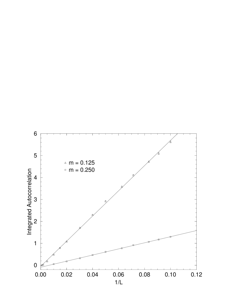
Figure 2: ${\cal A}_{{\cal M}^{2}}$ for lexicographic updates in one dimension with $m=0.125$ and $0.250$ at $\zeta=\zeta_{c}$. The error bars are smaller than the symbols.

3.2.4 Random Lexicographic Updates

On physical grounds it is obvious that the effect of surface terms on behaviour of ${\cal A}_{\Omega}$ for any quantity $\Omega$ will go to zero, typically as $1/L$, in the limit of large volumes. A periodic lattice does not have any boundaries, it is only the updating scheme that introduces a boundary as the collection of points at which the lexicographic property is violated; for this reason expressions describing autocorrelations do not have exact translational invariance. An obvious way to enhance translational invariance is to randomize the choice of starting point for each sweep through the lattice. For this case we are able to provide a relatively simple direct proof that surface effects only give small corrections to the integrated autocorrelation even for quadratic operators.

The boundary is completely specified by the site that is updated first in the sweep; if $x\equiv(x_{1},x_{2},\cdots,x_{d})$ is this first site then a site $y$ belongs to the boundary if $y_{j}=x_{j}$ or $y_{j}=x_{j+L-1}$ for at least one $j$. We thus need to give every lattice site an equal chance of being the starting point of the lexicographic chain.

Consider the representation of lexicographic updates in terms of the local update matrices (6)

$$M=M_{x_{L^{d}}}M_{x_{L^{d}-1}}\cdots M_{x_{2}}M_{x_{1}},$$

where the sequence $x_{1},x_{2},\ldots,x_{L^{d}}$ defines the lexicographic ordering. If we relabel the sites by a lattice translation $x\mapsto x-a$ and apply the same lexicographic update in the new coordinates then in the old coordinates this corresponds to choosing the initial site to be $x_{1}+a$ and the update matrix to be

$$M^{(a)}=M_{x_{L^{d}}+a}M_{x_{L^{d}-1}+a}\cdots M_{x_{2}+a}M_{x_{1}+a}.$$

The matrix $M_{x+a}$ can be written in the form

$$M_{x+a}=S^{(a)}M_{x}S^{(-a)},\qquad S^{(a)}_{x,y}\equiv\delta_{x,y+a}.$$

Using the composition property $S^{(a)}S^{(b)}=S^{(a+b)}$ we have

$$M^{(a)}=S^{(a)}MS^{(-a)}.$$

We now propose the updating scheme where before any given sweep, this relabelling of sites is performed at random. In other words, the translation vector $a$ will be a random variable, uniformly distributed over ${\twelvebb Z}_{L}^{d}$. The linear update matrix averaged over these translations is given by

$$\bar{M}={1\over L^{d}}\sum_{a\in{\twelvebb Z}_{L}^{d}}S^{(a)}MS^{(-a)}.$$

In Fourier space we have

$$S^{(a)}_{p,q}=\delta_{p,q}e^{-i{2\pi\over L}p\cdot a},\qquad\mbox{and}\qquad\bar{M}_{p,q}=\delta_{p,q}M_{p,q};$$

as expected, the linear update matrix retains only the diagonal part of $M$.

The quadratic update matrix in the $\{\phi_{p}^{*}\phi_{q}\}$ basis is similarly given by

$$\bar{M}^{Q}={1\over L^{d}}\sum_{a\in{\twelvebb Z}_{L}^{d}}(S^{(a)}MS^{(-a)})^{*}\otimes(S^{(a)}MS^{(-a)}).$$

Performing the sum over translations yields

$$\bar{M}^{Q}_{pq,rs}=M_{p,r}^{*}M_{q,s}\delta_{p-q,r-s},$$

implying that the quadratic monomial $\phi_{p}^{*}\phi_{q}$ couples only to monomials $\phi_{r}^{*}\phi_{s}$ satisfying $p-q=r-s$. Restricting ourselves to the sector with $p-q=0$ and defining $\Phi_{p}\equiv\phi_{p}^{*}\phi_{p}$ we have

$$\Phi^{\prime}=\bar{M}^{Q,0}\Phi,\qquad\mbox{with}\qquad\bar{M}^{Q,0}_{p,q}=M_{p,q}^{*}M_{p,q};$$

here $\bar{M}^{Q,0}$ is the corresponding $L^{d}\times L^{d}$ block of the quadratic update matrix given by the Hadamard product $M^{*}\cdot M$. We are interested in showing that

$$1+{\cal A}_{{\cal M}^{2}}=({\twelvebb I}-M^{*}\cdot M)^{-1}_{0,0}\to({\twelvebb I}-{M^{D}}^{*}\cdot M^{D})^{-1}_{0,0}\qquad\mbox{as $L\to\infty$.}$$ (31)

Let us start by writing the matrix $M$ explicitly as (19)

$$M=M^{D}+\sum_{l=1}^{d}{1\over L^{l}}G^{(l)},$$

where we have absorbed the exponentially small corrections into the matrices $G^{(l)}$; we then have a decomposition

$${\twelvebb I}-M^{*}\cdot M={\twelvebb I}-{M^{D}}^{*}\cdot M^{D}-E^{(1)}-E^{(2)}\equiv{\twelvebb I}-{M^{D}}^{*}\cdot M^{D}-E,$$

where

$$E^{(1)}_{p,q} = M^{D}_{p,q}\sum_{l=1}^{d}{1\over L^{l}}{G^{(l)}_{p,q}}^{*}+{M^{D}_{p,q}}^{*}\sum_{l=1}^{d}{1\over L^{l}}G^{(l)}_{p,q}$$ (32)

$$E^{(2)}_{p,q} = \sum_{j,l=1}^{d}{1\over L^{l+j}}{G^{(l)}_{p,q}}^{*}G^{(j)}_{p,q}=\sum_{j,l=1}^{d}\sum_{\scriptstyle\{\mu_{1},\ldots,\mu_{l}\}\atop\scriptstyle\{\nu_{1},\ldots,\nu_{j}\}}{1\over L^{l+j}}\delta_{p,q}^{\mu_{1},\ldots,\mu_{l}}\delta_{p,q}^{\nu_{1},\ldots,\nu_{j}}\left.{\hat{G}}^{\mu_{1},\ldots,\mu_{l}}_{p,q}\right.^{*}{\hat{G}}^{\nu_{1},\ldots,\nu_{j}}_{p,q}.$$ (33)

We now argue that the “error” matrix $E$ is small at large volumes in the sense that its matrix norm tends to zero in that limit. To show this we use the maximum sum row norm $\|A\|\equiv\max_{p}\sum_{q}|A_{p,q}|$. Consider first $E^{(1)}$, which is a diagonal matrix since $M^{D}$ is diagonal; the matrix elements of $M^{D}$ and $G^{(l)}$ are bounded by $L$-independent constants, thus there is a constant $C_{1}$ such that $\|E^{(1)}\|\leq C_{1}/L$ for all $L$. Turning to $E^{(2)}$, since there are an $L$-independent number of terms in equation (33), it suffices to consider the norm of a general term in that sum. We have

$$\sum_{q}{1\over L^{l+j}}\delta_{p,q}^{\mu_{1},\ldots,\mu_{l}}\delta_{p,q}^{\nu_{1},\ldots,\nu_{j}}\left|\left.\hat{G}^{\mu_{1},\ldots,\mu_{l}}_{p,q}\right.^{*}\hat{G}^{\nu_{1},\ldots,\nu_{j}}_{p,q}\right|<{C^{2}\over L^{l+j-k}}\leq{C^{2}\over L},$$ (34)

where $k$ is the cardinality of the set $\{\mu_{1},\ldots,\mu_{l}\}\cap\{\nu_{1},\ldots,\nu_{j}\}$; we have again used the fact that the matrix elements of the matrices $\hat{G}^{\mu_{1},\ldots,\mu_{l}}$ have an $L$-independent bound $|\hat{G}^{\mu_{1},\ldots,\mu_{l}}_{p,q}|<C$. The last inequality in (34) follows from the fact that $k\leq\min(l,j)$ and consequently $l+j-k\geq 1$. We have thus established that $\|E^{(2)}\|\leq C_{2}/L$ for all $L$. Putting the two bounds together we have

$$\|E\|\leq{C_{1}+C_{2}\over L}\equiv{C_{3}\over L}.$$

As the final ingredient we use the standard formula for the error in the inverse, namely

$$\left\|(A-E)^{-1}-A^{-1}\right\|\leq{\|A^{-1}\|^{2}\over 1-\|A^{-1}E\|}\|E\|;$$ (35)

this is valid for any matrix $A$ and “error” $E$ and any norm in which $\|A^{-1}E\|<1$.

Let $A\equiv{\twelvebb I}-{M^{D}}^{*}\cdot M^{D}$, then $\|A^{-1}\|$ has an $L$-independent upper bound and $\lim_{L\to\infty}\|E\|=0$, so we have $\|A^{-1}E\|\leq\|A^{-1}\|\cdot\|E\|<1$ for sufficiently large $L$. Formula (35) is thus applicable, and

$$\left\|({\twelvebb I}-M^{*}\cdot M)^{-1}-({\twelvebb I}-{M^{D}}^{*}\cdot M^{D})^{-1}\right\|\leq{C_{4}\over L},$$ (36)

for sufficiently large $L$; the required result (31) follows.

In the infinite volume limit ${\cal A}_{\cal M}^{2}$ is the same as for the standard lexicographic update (25). Whilst equation (36) tells us that the leading finite volume correction is at worst $O(1/L)$, it is actually $O(1/L^{2})$ at $\zeta=\zeta_{c}$. Indeed, the matrix elements of $E^{(2)}$ are supressed by $1/L^{2}$ and consequently the $O(1/L)$ part is determined solely by $E^{(1)}$, which is diagonal. Using the explicit form (22) of matrix $G^{(1)}$ this leading correction can be evaluated, and the correction vanishes at $\zeta=\zeta_{c}$. The $1/L^{2}$ behaviour of the correction is in accord with numerical results, as shown in Figure 3.

Figure 3: ${\cal A}_{{\cal M}^{2}}$ for random lexicographic updates in one dimension with $m=0.25$ at $\zeta=\zeta_{c}$. The $1/L^{2}$ fit was made to the leftmost six points, but not constrained to go through the origin.

3.3 Random Updates

Finally consider an updating scheme in which the sites to be updated are chosen at random. A sequence of $L^{d}$ such local updates will be called a “sweep”.

For a single site update we use the update matrix $M_{z}$ given in equation (5) with the updated site $z$ being a random variable, uniformly distributed over ${\twelvebb Z}_{L}^{d}$. In Fourier space we obtain

$$(M_{z})_{p,q}=\delta_{p,q}+{1\over L^{d}}e^{-2\pi i(p-q)z/L}f(q),$$

with

$$f(q)=\zeta\biggl{[}{2\over\omega^{2}}\sum_{\mu=1}^{d}\cos{2\pi\over L}q_{\mu}-1\biggr{]}.$$

For autocorrelations of quadratic operators we define the quadratic elementary update matrix $M_{z}^{Q}$ in basis $(\phi_{p}^{*}\phi_{q})$, namely

$$(M_{z}^{Q})_{pq,rs}=(M_{z}^{*}\otimes M_{z})_{pq,rs}=(M_{z})_{p,r}^{*}(M_{z})_{q,s}.$$

3.3.1 Autocorrelations for ${\cal M}$

The linear update matrix for a random update sweep, $M$, averaged over the independent random variables $z_{i}$ is given by

$$M=\prod_{i=1}^{L^{d}}\biggl{(}{1\over L^{d}}\sum_{z_{i}=1}^{L^{d}}M_{z_{i}}\biggr{)}=\biggl{(}{1\over L^{d}}\sum_{z=1}^{L^{d}}M_{z}\biggr{)}^{L^{d}}.$$

Explicitly, we have

$$M_{p,q}=\delta_{p,q}\left(1+{f(q)\over L^{d}}\right)^{L^{d}}=\delta_{p,q}e^{f(q)}\left(1-{f(q)^{2}\over 2L^{d}}+O\left({1\over L^{2d}}\right)\right),$$

giving the integrated autocorrelation

$$1+{\cal A}_{\cal M}=[{\twelvebb I}-M]^{-1}_{0,0}={1\over 1-\exp\left(-{\zeta m^{2}\over m^{2}+2d}\right)}+{\zeta^{2}m^{4}\over L^{d}8(m^{2}+2d)^{2}\sinh^{2}\left({\zeta m^{2}\over 2(m^{2}+2d)}\right)}+O\left({1\over L^{2d}}\right).$$

In the small mass limit we have

$$1+{\cal A}_{\cal M}={2d\over\zeta m^{2}}+O(m^{0}),$$

indicating that $z_{\cal M}=2$ regardless of the choice of $\zeta$. Even though the modes have completely decoupled and the autocorrelation function is a single exponential, the random choice of the site to be updated completely destroys the coherence and the algorithm cannot be tuned to reduce the critical slowing down.

3.3.2 Autocorrelations for ${{\cal M}^{2}}$

The quadratic update matrix $M^{Q}$ averaged over the random variables $z_{i}$ is

$$M^{Q}=\prod_{i=1}^{L^{d}}\biggl{(}{1\over L^{d}}\sum_{z_{i}=1}^{L^{d}}M^{Q}_{z_{i}}\biggr{)}=\biggl{(}{1\over L^{d}}\sum_{z=1}^{L^{d}}M^{Q}_{z}\biggr{)}^{L^{d}}.$$ (37)

Straightforward evaluation gives

$${1\over L^{d}}\sum_{z=1}^{L^{d}}M^{Q}_{z}={\twelvebb I}+{1\over L^{d}}\left(D^{Q}+{1\over L^{d}}C^{Q}\right),$$

with

$$D^{Q}_{pq,rs}=\delta_{p,r}\delta_{q,s}\bigl{(}f(r)+f(s)\bigr{)},\qquad C^{Q}_{pq,rs}=\delta_{p-r,q-s}f(r)f(s).$$

Inserting this into equation (37) yields

$$M^{Q}=\exp(D^{Q})+O\left({1\over L^{d}}\right);$$

we have not evaluated the $O(1/L^{d})$ correction in this case. In the infinite volume limit we obtain

$$[{\twelvebb I}-M^{Q}]^{-1}_{pq,rs}={\delta_{p,r}\delta_{q,s}\over 1-e^{f(r)+f(s)}},$$

and the integrated autocorrelation of ${{\cal M}^{2}}$ is given by

$$1+{\cal A}_{{\cal M}^{2}}={1\over 1-\exp\left(-{2\zeta m^{2}\over m^{2}+2d}\right)}\approx{d\over\zeta m^{2}}+O(m^{0})\qquad\mbox{for $m\to 0$}.$$

We therefore find that again that the algorithm with random updates cannot be tuned to reduce critical slowing down below $z_{{\cal M}^{2}}=2$.

4 Conclusions

The principal lesson which we may draw from this analysis is that it is possible to reduce the cost of a Local Hybrid Monte Carlo computation by a judicious choice of the order in which the variables are updated, as well as a careful tuning of the amount of randomness which is introduced into the system. While this differs from some previous claims, it is similar to the situation for deterministic Gauss-Seidel linear equation solvers.

The relevant autocorrelation for the determination of the cost is the integrated autocorrelation, and it is in terms of this autocorrelation that we define the critical exponent ${z_{\mbox{\tiny int}}}$. Furthermore, we define ${z_{\mbox{\tiny int}}}$ by ${\cal A}\propto\xi^{z_{\mbox{\tiny int}}}$ as $L,\xi\to\infty$ and $\xi/L\to 0$. This is to be contrasted with a finite size scaling analysis in which the limits are taken in a different order. For a zero temperature quantum field theory our choice of limits seems more natural.

Most local algorithms are special cases of LHMC, so our analysis is of fairly general applicability if we assume that the behaviour of autocorrelations in asymptotically free interacting theories is similar to that of free field theory. We intend to study this empirically in a future publication.

Of course local algorithms are directly applicable only to theories with local bosonic actions, but they are used within some dynamical fermion algorithms such as that proposed by Lüscher [20].

One issue of practical importance which has not been addressed at all in this paper is the difficulty of implementing the lexicographic scheme on parallel computers. Nevertheless it may well be advantageous to use a local lexicographic scheme on parallel computers, as has been suggested for the case of preconditioning conjugate gradient linear equation solvers [21].

Appendix A Calculation of $M$ in the Lexicographic Scheme

Our aim in this section is to show that the update matrix $M$ for lexicographic updates has the structure as given in equation (19), with the leading term of equation (21) and subleading term of equation (22). We shall prove this by induction in the number of dimensions $d$ for fixed lattice size $L$. The update matrix is a function of the mass and the overrelaxation parameter as well as $d$ and $L$, $M^{(d)}=M^{(d)}(m,\zeta)$. The induction step assumes that $M^{(d)}$ is known for all $m>0$ and $0<\zeta<2$ and relates $M^{(d+1)}(m,\zeta)$ to $M^{(d)}(m^{\prime},\zeta)$.

Consider the vector of field variables $\phi\equiv(\phi_{1},\phi_{2},\ldots,\phi_{L})$ in $d+1$ dimensions, where we only keep the index corresponding to the new dimension $d+1$, that is, $\phi_{x}$ is itself a vector of field variables in $d$ dimensions. We first find the matrix $M^{(d+1)}_{z}$, corresponding to lexicographic update of the variables $\phi_{z}$ only. Separating the dependence on the “old” and “new” variables in this subspace as usual, we obtain

$$\phi_{z}^{\prime}=O^{(d)}\phi_{z}+N^{(d)}\phi_{z}^{\prime}+{\twelvebb I}{\zeta\over\omega^{2}}(\phi_{z+1}-\phi_{z-1}),$$

or

$$\phi_{z}^{\prime}=M^{(d)}\phi_{z}+({\twelvebb I}-N^{(d)})^{-1}{\zeta\over\omega^{2}}(\phi_{z+1}-\phi_{z-1}).$$

We emphasise that the system under consideration is $d+1$ dimensional, and so $\omega^{2}=m^{2}+2(d+1)$; furthermore the update matrix $M^{(d)}$ for a $d$-dimensional subspace is the same as that for a $d$-dimensional system with mass ${m^{\prime}}^{2}=2+m^{2}$. For convenience we define a variable $t\equiv\zeta/\omega^{2}$; and we consider $N^{(d)}$ to be a function of $t$, and $O^{(d)}$ and $M^{(d)}$ to be functions of both $t$ and $\zeta$. We can thus write

$$\left[M_{z}^{(d+1)}\right]_{x,y}={\twelvebb I}\delta_{x,y}+\delta_{y,z}\Bigl{[}(M^{(d)}-{\twelvebb I})\delta_{x,y}+t({\twelvebb I}-N^{(d)})^{-1}(\delta_{x+1,y}+\delta_{x-1,y})\Bigr{]}.$$

The full update matrix is the product (in lexicographic order) of the subspace update matrices. In particular,

$$M^{(d+1)}=M_{L}^{(d+1)}M_{L-1}^{(d+1)}\ldots M_{1}^{(d+1)}=(M_{L}^{(d+1)}S)^{L}\equiv(\hat{M}_{L}^{(d+1)})^{L},$$

where $S_{x,y}\equiv{\twelvebb I}\delta_{x,y-1}$ represents a translation in the new coordinate $d+1$.

In Fourier space it is convenient to introduce $\alpha\equiv e^{2\pi i/L}$, so we have

$$\left[{\hat{M}}_{L}^{(d+1)}\right]_{p,q}=\left\{{\twelvebb I}\delta_{p,q}+{1\over L}\Bigl{[}M^{(d)}-{\twelvebb I}+t({\twelvebb I}-N^{(d)})^{-1}(\alpha^{q}+\alpha^{-q})\Bigr{]}\right\}\alpha^{q}.$$

Note that we only show the indices corresponding to the new dimension. Writing $T\equiv t({\twelvebb I}-N^{(d)})^{-1}$ one can show by induction that the matrix elements of the $l$th power for $l<L$ are given by

$$\left[\left.{\hat{M}}_{L}^{(d+1)}\right.^{l}\right]_{p,q}=\left\{{\twelvebb I}\delta_{p,q}\alpha^{q(l-1)}+{1\over L}{\cal P}_{l-1}(\alpha^{p},\alpha^{q},T)\Bigl{[}M^{(d)}-{\twelvebb I}+t({\twelvebb I}-N^{(d)})^{-1}(\alpha^{q}+\alpha^{-q})\Bigr{]}\right\}\alpha^{q},$$

with

$${\cal P}_{l}(x_{1},\ldots,x_{n})=\sum_{m_{1},\ldots,m_{n}\geq 0\atop m_{1}+\cdots+m_{n}=l}x_{1}^{m_{1}}\ldots x_{n}^{m_{n}},$$

which satisfies the following useful identities

$${\cal P}_{l}(x_{1},\ldots,x_{n}) = \sum_{j=0}^{l}x_{n}^{j}{\cal P}_{l-j}(x_{1},\ldots,x_{n-1})$$

$${\cal P}_{l}(x_{1},\ldots,x_{n}) = x_{n}{\cal P}_{l-1}(x_{1},\ldots,x_{n})+{\cal P}_{l}(x_{1},\ldots,x_{n-1})$$

$${\cal P}_{l}(x,y) = {x^{l+1}-y^{l+1}\over x-y}.$$

The $L$th power has one extra term giving

$$\left[M^{(d+1)}\right]_{p,q}={\twelvebb I}\delta_{p,q}+{\alpha^{q}\over L}\Bigl{[}{\cal P}_{L-1}(\alpha^{p},\alpha^{q},T)+T\Bigr{]}\Bigl{[}M^{(d)}-{\twelvebb I}+t({\twelvebb I}-N^{(d)})^{-1}(\alpha^{q}+\alpha^{-q})\Bigr{]}.$$ (38)

We can obtain a simpler recursion relation for $({\twelvebb I}-N)^{-1}$, which is related to $M$ through multiplication by the diagonal matrix; indeed, using equations (30) and (16) we get from (38)

$$\left[\Bigl{(}{\twelvebb I}-N^{(d+1)}\Bigr{)}^{-1}\right]_{p,q}={\alpha^{q}\over L}\Bigl{[}{\cal P}_{L-1}(\alpha^{p},\alpha^{q},T)+T\Bigr{]}\Bigl{(}{\twelvebb I}-N^{(d)}\Bigr{)}^{-1}.$$ (39)

Finally we need to transform ${\cal P}_{L-1}(\alpha^{p},\alpha^{q},T)$ into an explicit form; straightforward algebraic manipulation leads to

$${\cal P}_{L-1}(\alpha^{p},\alpha^{q},T)=\delta_{p,q}L(\alpha^{p}{\twelvebb I}-T)^{-1}-T(\alpha^{p}{\twelvebb I}-T)^{-1}(\alpha^{q}{\twelvebb I}-T)^{-1}({\twelvebb I}-T^{L}).$$ (40)

Recalling the definition of $T$ we have also

$$(\alpha^{p}{\twelvebb I}-T)^{-1}={\alpha^{-p}\over 1-t\alpha^{-p}}\left({\twelvebb I}-{1\over 1-t\alpha^{-p}}N^{(d)}\right)^{-1}({\twelvebb I}-N^{(d)}).$$ (41)

It is important to note here that the inverse on the right of this equation exists: we know that $({\twelvebb I}-N^{(d)})^{-1}$ exists for all $|t|<1/d$, where $t$ enters as a multiplicative factor in definition of $N^{(d)}$ (see equations (16)—(18)). However, in $d+1$ dimensions $t$ satisfies a more stringent constraint, namely $t<1/(d+1)$, and consequently

$$\left|{t\over 1-t\alpha^{-p}}\right|\leq\left|{t\over 1-t}\right|<{1\over d},$$

implying the existence of $({\twelvebb I}-{1\over 1-t\alpha^{-p}}N^{(d)})^{-1}$ for all $p$. Inserting relations (40) and (41) into equation (39) we get an explicit recursion relation

$$\Bigl{[}{\twelvebb I} - N^{(d+1)}\Bigr{]}^{-1}_{p,q}=\delta_{p,q}{1\over 1-t\alpha^{-p}}\left({\twelvebb I}-{1\over 1-t\alpha^{-p}}N^{(d)}\right)^{-1}$$ (42)

$$- {t\over L}\Bigl{(}{\twelvebb I}-T^{L}\Bigr{)}{\alpha^{-p}\over(1-t\alpha^{-p})(1-t\alpha^{-q})}\left({\twelvebb I}-{1\over 1-t\alpha^{-p}}N^{(d)}\right)^{-1}\left({\twelvebb I}-{1\over 1-t\alpha^{-q}}N^{(d)}\right)^{-1}$$

$$+ {t\over L}\alpha^{q}\left({\twelvebb I}-N^{(d)}\right)^{-2}.$$

In principle this allows us to calculate the update matrix in any dimension. Consider building a $1$-dimensional update matrix from single site updates ($d=0$); Obviously, $N^{(0)}\equiv 0$ and the recursion relation gives the exact result

$$\left[{\twelvebb I}-N^{(1)}\right]^{-1}_{p,q}={\delta_{p,q}\over 1-t\alpha^{-p}}+{t\over L}\left[\alpha^{q}-{\alpha^{-p}(1-t^{L})\over(1-t\alpha^{-p})(1-t\alpha^{-q})}\right].$$ (43)

Note that the above result has the expected structure and the leading term exactly corresponds to $[{\twelvebb I}-{N^{(1)}}^{D}]^{-1}$ with ${N^{(d)}}^{D}$ denoting a diagonal part of $N^{(d)}$, defined in (17). Using $N^{(1)}$ we can calculate $N^{(2)}$ etc. The only problem from the practical point of view is the calculation of $T^{L}=t^{L}[({\twelvebb I}-N^{(d)})^{-1}]^{L}$. However, since $t<1$ this term is exponentially small in $L$ and can be neglected at large volumes. Similarly, the exponentially small terms will be generated (and can be neglected) from matrix multiplications in the recursion relation when using, e.g., the Poisson resummation formula for the matrix elements of the product.

While the above program can be carried out to arbitrary number of dimensions, it is sufficient for our purposes to deduce the structure that follows from equations (42) and (43). Indeed, one can easily verify the following conclusions:

1. In any number of dimensions we have

   $$\left[{\twelvebb I}-N\right]^{-1}=\sum_{l=0}^{d}{1\over L^{l}}K^{(l)}+O\left({1\over L}t^{L}\right).$$

   The matrix elements of $K^{(l)}$ are bounded by an $L$-independent bound and have the form

   $$K^{(l)}_{p,q}=\sum_{\{\mu_{1},\ldots,\mu_{l}\}}\delta_{p,q}^{\mu_{1},\ldots,\mu_{l}}\hat{K}^{\mu_{1},\ldots,\mu_{l}}_{p,q},$$

   where the modified delta function is defined in equation (20), and $\{\mu_{1},\ldots,\mu_{l}\}$ represents any subset of integers $\{1,\ldots,d\}$ with $l$ elements. This follows from the (43) and the fact that the above structure is invariant with respect to recursion relation (42). Note that the exponentially small terms could also be included in matrices $K^{(l)}$, but we keep them separately for the practical reasons mentioned above.

2. The invariant form of the leading term is given by

   $$\hat{K}_{p,q}={1\over\displaystyle{1-t\sum_{\mu}\alpha^{-p_{\mu}}}},$$

   which corresponds to $[{\twelvebb I}-N^{D}]^{-1}$ as expected.

3. The invariant form of the first finite volume correction is

   $$\hat{K}^{\mu}_{p,q}=t\left[{\alpha^{q_{\mu}}\over\displaystyle{\Bigl{(}1-t\sum_{\nu\neq\mu}\alpha^{-p_{\nu}}\Bigr{)}\Bigl{(}1-t\sum_{\epsilon\neq\mu}\alpha^{-q_{\epsilon}}\Bigr{)}}}-{\alpha^{-p_{\mu}}\over\displaystyle{\Bigl{(}1-t\sum_{\nu}\alpha^{-p_{\nu}}\Bigr{)}\Bigl{(}1-t\sum_{\epsilon}\alpha^{-q_{\epsilon}}\Bigr{)}}}\right].$$ (44)

   The corresponding forms for the update matrix $M$ are given in equations (19-22).

Appendix B Boundedness of Finite Volume Corrections

In this appendix we show that the surface corrections for the lexicographic updating scheme do indeed go to zero as the inverse of the lattice size. For the case of quadratic operators we shall assume that the infinite volume limit of $\det({\twelvebb I}-M^{*}\otimes M)\neq 0$: we have not yet found a simple proof of this, although it would follow trivially from a proof of the ergodicity of the LHMC algorithm in an infinite volume.

The basic idea of the proof is to expand about the infinite volume limit, and thus our proof is naturally expressed in the language of functional analysis. Our argument is essentially that the update operator $M$ is a compact (completely continuous) operator on the Hilbert space $L^{2}([0,2\pi])$ — in fact in one dimension it is a Hilbert-Schmidt kernel — and that the finite volume results may be expanded about the infinite volume ones using the Poisson resummation formula. We have chosen to prove our results following the original method of Fredholm, as this seems to be the most direct approach [22].

We start by proving a simple bound on determinants:

Lemma 1 (Hadamard)

For any matrix $A:l^{2}_{k}({\twelvebb C})\to l^{2}_{k}({\twelvebb C})$

$$|\det A|\leq\prod_{i}\|A_{i}\|$$

where $A_{i}$ is a row of $A$ and $\|A_{i}\|^{2}=\sum_{j}|A_{ij}|^{2}$ is its norm.

Proof. If $A$ has any row which is zero then the inequality is trivially satisfied. Otherwise construct a new matrix $B$ whose rows are $B_{i}=A_{i}/\|A_{i}\|$, then the bound is equivalent to $|\det B|\leq 1$ for all complex matrices whose rows are normalized. If the rows of $B$ are not all orthogonal then there are two rows $u$ and $v$ such that $|(u,v)|>0$, $\|u\|=\|v\|=1$. If we replace the row $v$ by $v^{\prime}\equiv v-(u,v)u$ then the determinant is unchanged, and $(u,v^{\prime})=0$. On the other hand $\|v\|^{2}=\|v^{\prime}+(u,v)u\|^{2}=\|v^{\prime}\|^{2}+|(u,v)|^{2}\|u\|^{2}$, so $\|v^{\prime}\|^{2}=1-|(u,v)|^{2}<1$; thus replacing the row $v^{\prime}$ by $v^{\prime\prime}\equiv v^{\prime}/\|v^{\prime}\|$ increases the determinant by a factor of $1/\|v^{\prime}\|>1$, and all the rows of the resulting matrix have unit length. This proves that the maximum value of the determinant must occur when the rows are orthonormal. If the rows of $B$ are orthonormal then $BB^{\dagger}=1$ and hence $\det BB^{\dagger}=\det B\det B^{\dagger}=\det B(\det B)^{*}=|\det B|^{2}=1$.   

Corollary 1

If all the elements of the matrix $A$ are bounded, $|A_{ij}|\leq C$, then $|\det A|\leq(C\sqrt{k})^{k}$.

Theorem 1 (Fredholm)

Let $\Delta:l^{2}_{L}({\twelvebb C})\to l^{2}_{L}({\twelvebb C})$ be a matrix all of whose elements are bounded by some ($L$-independent) constant $|\Delta_{ij}|\leq C$; then $\left|\det\left({\twelvebb I}+{1\over L}\Delta\right)\right|\leq C^{\prime}$ where $C^{\prime}$ is a constant which is independent of $L$.

Proof. Let us introduce a parameter $\lambda$ and then expand in powers of $\lambda$ to obtain

$$\left|\det\left(1+{\lambda\over L}\Delta\right)\right|=\left|\sum_{k=0}^{L}\left(\lambda\over L\right)^{k}\sum_{i_{1}>i_{2}>\cdots>i_{k}}\det\left(\begin{array}[]{ccc}\Delta_{i_{1}i_{1}}&\ldots&\Delta_{i_{1}i_{k}}\\ \vdots&\ddots&\vdots\\ \Delta_{i_{k}i_{1}}&\ldots&\Delta_{i_{k}i_{k}}\\ \end{array}\right)\right|,$$

using Hadamard’s bound

$$\leq\,\sum_{k=0}^{L}\left(\lambda\over L\right)^{k}\sum_{i_{1}>i_{2}>\cdots>i_{k}}(C\sqrt{k})^{k}\,=\,\sum_{k=0}^{L}\left(\lambda\over L\right)^{k}{L\choose k}(C\sqrt{k})^{k}\,\leq\,\sum_{k=0}^{\infty}{(\lambda C\sqrt{k})^{k}\over k!}\,=\,C^{\prime}(\lambda)$$

where the ratio test may be applied to show that the series converges for all $\lambda$. The desired result follows upon setting $\lambda=1$.   

Definition 1

The minor $\Delta^{(ij)}$ of a matrix $\Delta$ is defined by

$$\Delta^{(ij)}_{kl}\equiv\left\{\begin{array}[]{cl}1&\mbox{if $k=i$ and $j=l$}\\ \Delta_{kl}&\mbox{if $k\neq i$ and $j\neq l$}\\ 0&\mbox{otherwise}\\ \end{array}\right.$$

Corollary 2 (Fredholm)

Let $\Delta$ be a matrix as in Theorem 1, then

$$\left|\det\left({\twelvebb I}+{1\over L}\Delta^{(ij)}\right)\right|\leq\left\{\begin{array}[]{cl}C^{\prime}&\mbox{if $i=j$}\\ C^{\prime}/L&\mbox{if $i\neq j$}\\ \end{array}\right.$$

where $C^{\prime}$ is an ($L$-independent) constant.

Proof. If $i=j$ then the matrix ${\twelvebb I}+{1\over L}\Delta^{(ij)}$ is of the form to which Theorem 1 is applicable. If $i\neq j$ then introducing the parameter $\lambda$ and expanding in powers of $\lambda$ as before we obtain

$$\left|\det\left(1+{\lambda\over L}\Delta^{(ij)}\right)\right|=\left|\sum_{k=0}^{L-2}\left(\lambda\over L\right)^{k+1}\sum_{{\scriptstyle i_{1}>i_{2}>\cdots>i_{k}\atop\scriptstyle i_{r}>i>i_{r+1}}\atop\scriptstyle i_{s}>j>i_{s+1}}(-1)^{r+s}\det\left(\begin{array}[]{cccc}\Delta_{ji}&\Delta_{ji_{1}}&\ldots&\Delta_{ji_{k}}\\ \Delta_{i_{1}i}&\Delta_{i_{1}i_{1}}&\ldots&\Delta_{i_{1}i_{k}}\\ \vdots&\vdots&\ddots&\vdots\\ \Delta_{i_{k}i}&\Delta_{i_{k}i_{1}}&\ldots&\Delta_{i_{k}i_{k}}\\ \end{array}\right)\right|,$$

using Hadamard’s bound

$$\leq \sum_{k=0}^{L-2}\left(\lambda\over L\right)^{k+1}\sum_{{\scriptstyle i_{1}>i_{2}>\cdots>i_{k}\atop\scriptstyle i_{r}>i>i_{r+1}}\atop\scriptstyle i_{s}>j>i_{s+1}}(C\sqrt{k+1})^{k+1}\,=\,\sum_{k=0}^{L-2}\left(\lambda\over L\right)^{k+1}{L-2\choose k}(C\sqrt{k+1})^{k+1}$$

$$\leq {1\over L}\sum_{k=0}^{\infty}{(\lambda C\sqrt{k+1})^{k+1}\over k!}\,=\,{C^{\prime}(\lambda)\over L}$$

where the ratio test may be applied to show that the series converges for all $\lambda$. The desired result follows upon setting $\lambda=1$.   

Definition 2

The adjoint $\mathop{\rm Adj}M$ of a matrix $M$ is defined to be the transpose of the matrix whose elements are the determinants of the corresponding minors, that is $(\mathop{\rm Adj}M)_{ij}\equiv\det M^{(ji)}$.

Theorem 2

Let $\Delta:l^{2}_{L}({\twelvebb C})\to l^{2}_{L}({\twelvebb C})$ be a matrix all of whose elements are bounded by some constant $|\Delta_{ij}|\leq C$, and $\det\left({\twelvebb I}+{1\over L}\Delta\right)\geq\alpha>0$ is bounded below by an ($L$-independent) constant, then $\left({\twelvebb I}+{1\over L}\Delta\right)^{-1}={\twelvebb I}+{1\over L}G$, where all the matrix elements of $G$ are bounded by an ($L$-independent) constant, $|G_{ij}|\leq C^{\prime\prime}$.

Proof. From the algebraic identity (Cramer’s rule)

$$\left({\twelvebb I}+{1\over L}\Delta\right)\mathop{\rm Adj}\left({\twelvebb I}+{1\over L}\Delta\right)=\det\left({\twelvebb I}+{1\over L}\Delta\right){\twelvebb I}\equiv D{\twelvebb I}$$

and the fact that $\left[\mathop{\rm Adj}\left({\twelvebb I}+{1\over L}\Delta\right)\right]_{ij}=C_{ij}/L$ for $i\neq j$ and $\left[\mathop{\rm Adj}\left({\twelvebb I}+{1\over L}\Delta\right)\right]_{jj}=C_{jj}$, which follow from Corollary 2, we have

$$\left(1+{1\over L}\Delta_{jj}\right)C_{jj}+\sum_{i\neq j}{1\over L^{2}}\Delta_{ji}C_{ij}=D.$$

From this we find that $C_{jj}=D+O(1/L)\Rightarrow C_{jj}/D=1+O(1/L)$, where we have made use of the fact that $D$ is bounded below by the constant $\alpha$. The desired result then follows from substituting this relation into Cramer’s rule above.   

Lemma 2

If the matrix elements $\Delta_{ij}$ referred to above are taken to be the values $\Delta\left({2\pi i\over L},{2\pi j\over L}\right)$ of a Lebesgue integrable function then we can define the infinite volume limit of the Fredholm determinant, and if this limit is non-zero then there must exist a non-zero constant $\alpha$ which bounds it from below.

Definition 3

Let $\alpha$ be a subset of the integers $\{1,\ldots,d\}$, and $\delta^{(\alpha)}_{pq}\equiv\prod_{\mu\not\in\alpha}\delta_{p_{\mu}q_{\mu}}$. A matrix $A$ has support on dimensions $\alpha$ if $A^{(\alpha)}_{pq}=\delta^{(\alpha)}_{pq}A_{pq}$, with $p$ and $q$ being a $d$-tuple of indices, $p=(p_{1},\ldots,p_{d})$.

Notice that according to our definition $A^{(\emptyset)}$ is a diagonal matrix.

Corollary 3

There is a permutation of the indices $p$ for each matrix $A^{(\alpha)}$ such that it is block diagonal with $\#\alpha\times\#\alpha$ blocks. Each block satisfies the assumptions of Theorem 2, so the inverse may be expressed in block diagonal form where each block is of the form specified in Theorem 2.

Lemma 3

If $A^{(\alpha)}$ has support on dimensions $\alpha$ and $B^{(\beta)}$ has support on dimensions $\beta$, and all the elements of are bounded by an ($L$-independent) constant, $|A^{(\alpha)}_{pq}|\leq C$ and $|B^{(\beta)}_{pq}|\leq C$, then

$$\sum_{q}L^{-\#\alpha}A^{(\alpha)}_{pq}L^{-\#\beta}B^{(\beta)}_{qr}=L^{-\#\alpha\cup\beta}W^{(\alpha\cup\beta)}_{pr}$$

where $W^{(\alpha\cup\beta)}$ has support on dimensions $\alpha\cup\beta$ and $|W^{(\alpha\cup\beta)}_{pr}|\leq C^{\prime}$. $\#\alpha$ is the cardinality of the set $\alpha$.

Proof. Consider the matrix product

$$\sum_{q}A^{(\alpha)}_{pq}B^{(\beta)}_{qr}=\sum_{q}A_{pq}B_{qr}\prod_{\mu\not\in\alpha\atop\nu\not\in\beta}\delta_{p_{\mu}q_{\mu}}\delta_{q_{\nu}r_{\nu}}.$$

The product of Kronecker tensors may be split into four disjoint classes, $\overline{\alpha\cup\beta}$, $\beta-\alpha$, $\alpha-\beta$, and $\alpha\cap\beta$:

$$\left(A^{(\alpha)}B^{(\beta)}\right)_{pr}=\sum_{q}A_{pq}B{qr}\left(\prod_{\mu\not\in\alpha\cup\beta}\delta_{p_{\mu}q_{\mu}}\delta_{q_{\mu}r_{\mu}}\right)\left(\prod_{\mu\in\beta-\alpha}\delta_{p_{\mu}q_{\mu}}\right)\left(\prod_{\mu\in\alpha-\beta}\delta_{q_{\mu}r_{\mu}}\right)\left(\prod_{\mu\in\alpha\cap\beta}1\right).$$

It is immediately apparent that only for $\mu$ in the last set of indices ($\alpha\cap\beta$) does the sum over $q_{\mu}$ have more than one non-vanishing term, and that for $\mu$ in the first set of indices ($\overline{\alpha\cup\beta}$) the expression vanishes unless $p_{\mu}=r_{\mu}$. We thus have

$$\left(A^{(\alpha)}B^{(\beta)}\right)_{pr}=\prod_{\mu\not\in\alpha\cup\beta}\delta_{p_{\mu}r_{\mu}}L^{\#\alpha\cap\beta}W_{pr},$$

with $|W_{pr}|\leq C^{\prime}$. The result now follows from the observation that $\#\alpha\cup\beta=\#\alpha+\#\beta-\#\alpha\cap\beta$.   

Theorem 3

Let $\Delta^{(\alpha)}$ be a matrix with support on dimensions $\alpha$ all of whose elements are bounded by an ($L$-independent) constant, and furthermore

$$\lim_{L\to\infty}\det\left({\twelvebb I}+\sum_{\alpha\neq\emptyset}L^{-\#\alpha}\Delta^{(\alpha)}\right)\neq 0;$$

then

$$\left({\twelvebb I}+\sum_{\alpha\neq\emptyset}L^{-\#\alpha}\Delta^{(\alpha)}\right)^{-1}={\twelvebb I}+\sum_{\alpha\neq\emptyset}L^{-\#\alpha}G^{(\alpha)}$$

where $G^{(\alpha)}$ its has support on dimensions $\alpha$ and all its elements bounded by a constant.

Proof. We may order the subsets of $\{1,\ldots,d\}$ lexicographically, that is $\alpha<\beta$ iff $\#\alpha<\#\beta$ or $\#\alpha=\#\beta$ and $\min_{i\in\alpha-\beta}i<\min_{j\in\beta-\alpha}j$. Let $\gamma$ be the smallest set for which $\Delta^{(\gamma)}\neq 0$. Then

$${\twelvebb I}+\sum_{\alpha\neq\emptyset}L^{-\#\alpha}\Delta^{(\alpha)}=\left({\twelvebb I}+L^{-\#\gamma}\Delta^{(\gamma)}\right)\left({\twelvebb I}+\left({\twelvebb I}+L^{-\#\gamma}\Delta^{(\gamma)}\right)^{-1}\sum_{\alpha>\gamma}L^{-\#\alpha}\Delta^{(\alpha)}\right).$$

The infinite volume limit of the determinant of this quantity is non zero, therefore the infinite volume limit of the determinant of each factor must be non zero. From Corollary 3 we have that $({\twelvebb I}+L^{-\#\gamma}\Delta^{(\gamma)})^{-1}={\twelvebb I}+L^{-\#\gamma}G^{(\gamma)}$ with $|G_{pq}|\leq C^{\prime}$, hence

$$\left({\twelvebb I}+\sum_{\alpha\neq\emptyset}L^{-\#\alpha}\Delta^{(\alpha)}\right)^{-1} = \left({\twelvebb I}+\left({\twelvebb I}+L^{-\#\gamma}G^{(\gamma)}\right)\sum_{\alpha>\gamma}L^{-\#\alpha}\Delta^{(\alpha)}\right)^{-1}\left({\twelvebb I}+L^{-\#\gamma}G^{(\gamma)}\right)$$

$$= \left({\twelvebb I}+\sum_{\alpha>\gamma}L^{-\#\alpha}{\Delta^{\prime}}^{(\alpha)}\right)^{-1}\left({\twelvebb I}+L^{-\#\gamma}G^{(\gamma)}\right)$$

$$= {\twelvebb I}+\sum_{\alpha\neq\emptyset}L^{-\#\alpha}{G^{\prime}}^{(\alpha)}$$

where we have used Lemmas 2 and 3, and the fact that $\alpha>\gamma\Rightarrow\alpha\cup\gamma>\gamma$ in the penultimate line. The final line follows by induction on $\gamma$.   

One application of these results uses the matrices $N$, $O$, $N^{D}$, $O^{D}$, and $R$ introduced in the body of the paper, and the matrix $\Delta$ defined as $\Delta\equiv({\twelvebb I}-N^{D})^{-1}R$.

Corollary 4

$M$ has the form given in equation (19).

Proof. Observe that

$${\twelvebb I}-N=\left({\twelvebb I}-N^{D}+{1\over L}R\right)=({\twelvebb I}-N^{D})\left({\twelvebb I}+{1\over L}({\twelvebb I}-N^{D})^{-1}R\right)=({\twelvebb I}-N^{D})\left({\twelvebb I}+{1\over L}\Delta\right);$$

since there is a basis in which $N$ is a strictly triangular matrix it follows that $\det({\twelvebb I}-N)=1\,(\forall L)$, and thus we may conclude that $\lim_{L\to\infty}\det\left({\twelvebb I}+{1\over L}\Delta\right)\neq 0$. Therefore $\Delta$ satisfies the assumptions of Theorem 3, so $\left({\twelvebb I}-{1\over L}\Delta\right)^{-1}$ has the desired form. From equation (30) we have

$$M={\twelvebb I}-({\twelvebb I}-N)^{-1}({\twelvebb I}-N^{D}-O^{D})={\twelvebb I}-\left({\twelvebb I}+{1\over L}\Delta\right)^{-1}({\twelvebb I}-N^{D})^{-1}({\twelvebb I}-N^{D}-O^{D}),$$

so we may apply Lemma 3 to show that $M$ also has the desired form.   

If the infinite volume Markov process has a unique fixed point then from equation (9) we obtain upon averaging over this fixed point distribution of $\phi$

$$({\twelvebb I}-M^{Q})\langle\phi^{Q}\rangle_{\phi,\pi}=P^{Q},$$

and the uniqueness of $\langle\phi^{Q}\rangle_{\phi,\pi}$ implies that $\lim_{L\to\infty}\det\left({\twelvebb I}-M^{*}\otimes M\right)\neq 0$. As a consequence of Corollary 4 we may write

$${\twelvebb I}-M^{*}\otimes M=\left({\twelvebb I}-{M^{D}}^{*}\otimes M^{D}\right)\left({\twelvebb I}+\sum_{\alpha}L^{-\#\alpha}A^{(\alpha)}\right),$$

where the matrix elements of $A^{(\alpha)}$ are bounded by an $L$-independent constant, and thus from Theorem 3 and Lemma 3 we may conclude that a result analogous to Corollary 4 applies to quadratic operators.

References

• [1] A. D. Kennedy, “Progress in lattice field theory algorithms,” in Smit and van Baal [23], pp. 96–107. Proceedings of the International Symposium on Lattice Field Theory, Amsterdam, the Netherlands, 15–19 September 1992.
• [2] S. L. Adler, “An Overrelaxation method for the Monte Carlo evaluation of the partition function for multiquadratic actions,” Phys. Rev. D23 (1981) 2901.
• [3] C. Whitmer, “Overrelaxation methods for Monte Carlo simulations of quadratic and multiquadratic actions,” Phys. Rev. D29 (1984) 306–311.
• [4] S. L. Adler, “Stochastic algorithm corresponding to a general linear iterative process,” Phys. Rev. Lett. 60 (1988) 1243.
• [5] S. L. Adler, “Overrelaxation algorithms for lattice field theories,” Phys. Rev. D37 (1988) 458.
• [6] H. Neuberger, “Adler’s overrelaxation algorithm for Goldstone bosons,” Phys. Rev. Lett. 59 (1987) 1877.
• [7] U. Wolff, “Dynamics of Hybrid Overrelaxation in the Gaussian model,” Phys. Lett. B288 (1992) 166–170.
• [8] J. Goodman and A. D. Sokal, “Multigrid Monte Carlo method. conceptual foundations,” Phys. Rev. D40 (Sept., 1989) 2035–2071.
• [9] G. Bathas and H. Neuberger, “A possible barrier at $z\approx 1$ for local algorithms,” Phys. Rev. D45 (1992) 3880–3883.
• [10] F. R. Brown and T. J. Woch, “Overrelaxed heat bath and Metropolis algorithms for accelerating pure gauge Monte Carlo calculations,” Phys. Rev. Lett. 58 (1987) 2394.
• [11] M. Creutz, “Overrelaxation and Monte Carlo simulation,” Phys. Rev. 36 (July, 1987) 515–519.
• [12] U. M. Heller and H. Neuberger, “Overrelaxation and mode coupling in $\sigma$ models,” Phys. Rev. D39 (1989) 616.
• [13] R. Petronzio and E. Vicari, “An Overrelaxed Monte Carlo algorithm for $SU(3)$ lattice gauge theories,” Phys. Lett. B245 (1990) 581–584.
• [14] A. D. Kennedy and K. M. Bitar, “An exact local Hybrid Monte Carlo algorithm for gauge theories,” in Lattice ’93 (T. Draper, S. Gottlieb, A. Soni, and D. Toussaint, eds.), vol. B34 of Nuclear Physics (Proceedings Supplements), pp. 786–788, Apr., 1994. hep-lat/9311017. Proceedings of the International Symposium on Lattice Field Theory, Dallas, Texas, 12–16 October 1993.
• [15] R. Gupta, G. W. Kilcup, A. Patel, S. R. Sharpe, and P. de Forcrand, “Comparison of update algorithms for pure gauge $SU(3)$,” Mod. Phys. Lett. A3 (1988) 1367–1378.
• [16] S. L. Adler and G. V. Bhanot, “Study of an overrelaxtion method for gauge theories,” Phys. Rev. Lett. 62 (Jan., 1989) 121–124.
• [17] J. Apostolakis, C. F. Baillie, and G. C. Fox, “Investigation of the two-dimensional $O(3)$ model using the overrelaxation algorithm,” Phys. Rev. D43 (1991) 2687–2693.
• [18] K. Akemi, P. de Forcrand, M. Fujisaki, T. Hashimoto, H. C. Hege, S. Hioki, O. Miyamura, A. Nakamura, M. Okuda, I. O. Stamatescu, Y. Tago, and T. Takaishi, “Autocorrelation in updating pure $SU(3)$ lattice gauge theory by the use of overrelaxed algorithms,” in Smit and van Baal [23], pp. 253–256. QCD–TARO Collaboration.
• [19] A. D. Kennedy and B. J. Pendleton, “Some exact results for Hybrid Monte Carlo.” In preparation, 1997.
• [20] M. Lüscher, “A new approach to the problem of dynamical quarks in numerical simulations of lattice QCD,” Nucl. Phys. B418 (1994) 637, hep-lat/9311007.
• [21] S. Fischer, A. Frommer, U. Glaessner, T. Lippert, G. Ritzenhoefer, and K. Schilling, “A parallel SSOR preconditioner for lattice QCD,” Comput. Phys. Commun. 98 (1996) 20–34, hep-lat/9602019.
• [22] F. Riesz and B. Szokefalvi-Nagy, Functional Analysis. Ungar, New York, 1955.
• [23] J. Smit and P. van Baal, eds., vol. B30 of Nuclear Physics (Proceedings Supplements), Mar., 1993. Proceedings of the International Symposium on Lattice Field Theory, Amsterdam, the Netherlands, 15–19 September 1992.