Multi-boson simulation of the Schrödinger functional

Abstract

We discuss the choice of parameters and report some results for unquenched simulations of the Schrödinger functional with a non-hermitean variant of Lüscher’s multi-boson algorithm.

Today Hybrid Monte Carlo (HMC) is the standard algorithm employed for simulations with dynamical fermions. In spite of its general success it seems desirable to have other methods at one’s disposal. In particular the multi-boson technique proposed by Lüscher [1] seems interesting. Apart from its theoretical appeal one may perform consistency checks and hope for better efficiency, in particular with regard to slow topological modes [2]. Better numerical stability and more flexibility in the treatment of statistical problems with exceptional configurations [3] may be further advantages. Soon after Lüscher’s proposal a non-hermitean variant of the algorithm has been advocated [4] and initial tests have been performed [5], which we extend here. Experiments with the original proposal are reported in [6].

The contribution to the QCD Boltzmann factor from two flavors of dynamical quarks is given by

$$\exp[-S_{\rm quarks}(U)]=\det(M)^{2}=|\det(M)|^{2},$$ (1)

where $M=M(U)$ is the (sofar unimproved) Wilson Dirac operator with the hermiticity property $M^{\dagger}=\gamma_{5}M\gamma_{5}$. For the multi-boson algorithm we employ a polynomial $P(M)$ which, over the spectrum of $M$, approximates the inverse,

$$|\det(M)|^{2}=|\det P(M)|^{-2}|\det(1-R(M))|^{2},$$ (2)

such that $R$ is a small remainder. This enables us to represent the dominant part of $S_{\rm quarks}$ as a bosonic path integral

$$|\det P(M)|^{-2}=$$

$$\int\mbox{\rm D}\phi\,\mbox{\rm D}\phi^{\dagger}\exp\Biggl{\{}-\sum_{kx}|(M-z_{k})\phi_{k}(x)|^{2}\Biggr{\}},$$ (3)

where $z_{k},k=1,\ldots,n$, are the roots of $P$. We now update by a sequence of

• some proposal $(U,\phi)\to(U^{\prime},\phi^{\prime})$ obeying detailed balance with respect to the sum of (3) and the gluon action

• acceptance with probability $q(R,R^{\prime},\chi)$,

where $R,R^{\prime}$ are the old and new remainders and $\chi$ is a complex random field governed by some probability distribution $\rho(\chi)$, in our case $\rho\propto\exp(-\chi^{\dagger}\chi)$. This compound can be proved to be a valid algorithm if

$$\frac{\langle q(R,R^{\prime},\chi)\rangle_{\chi}}{\langle q(R^{\prime},R,\chi)\rangle_{\chi}}=|\det(W)|^{-2}$$ (4)

with $W=(1-R^{\prime})^{-1}(1-R)$ holds stochastically (i.e. averaged over $\chi$). A simple (non-stochastic) solution would be

$$q_{0}=\min(1,|\det W|^{-2}).$$ (5)

It requires the computation of the det of $W$. We here use the “noisy algorithm” of [4] corresponding to

$$q=\min\left(1,\frac{\rho(W\chi)}{\rho(\chi)}\right).$$ (6)

To evaluate $q$ the application of $W$ to vectors suffices, and the required inversion of $1-R^{\prime}$ with some inverter like BiCGstab is rather uncritical. For completeness we mention that the variant called “non-noisy” in [5] was found incorrect in the implementation described there.

Following [4] we construct $P$ by using Chebyshev polynomials for $R$. On families of nested ellipses with centers at $d$,

$$z(\theta,\varphi)=d-e\cosh(\theta+i\varphi),$$ (7)

they approximate the inverse with a rate $|R|\leq\exp(-(n+1)(\theta_{0}-\theta))$. Here $d,e$ are fixed parameters, $\theta$ labels the ellipses and $\varphi\in[0,2\pi)$ traces them. The polynomial is determined (up to a factor) by the roots $z_{k}=z(\theta_{0},2\pi k/(n+1)),k=1,2,\ldots,n$, lying on the ellipse passing through the origin, $e\cosh\theta_{0}=d$. Due to even-odd symmetry, the spectrum of $M$ is symmetric under $\lambda\to 2-\lambda$ and we hence set $d=1$.

To implement the correction step we have to evaluate $R\chi$. The factorized form, $1-R=c_{n}M\prod(M-z_{k})$, tends to be numerically unstable [3, 7]. Here it can be avoided and replaced by a uniformly stable two step recursion starting from $\chi_{0}=\chi$ and leading to $\chi_{n+1}=R\chi$. It is straightforwardly based on the standard recurrence for Chebyshev polynomials. The intermediate $\chi_{k}$ are the remainders for lower degree polynomials. We follow the recursion to investigate the choice of degree $n$ and the focal distance $e$. With some trial parameters we produced some equilibrated $U$-configurations, and for one of them Figs.1,2 show the quality of approximation.

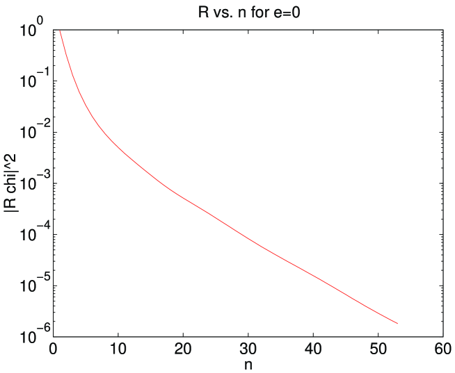
Figure 1: Remainder of the inversion with $e=0$ for the Schrödinger functional, $L=T=4,\beta=6.4,K=0.15,\theta=\pi/5$, background field “A”[9]

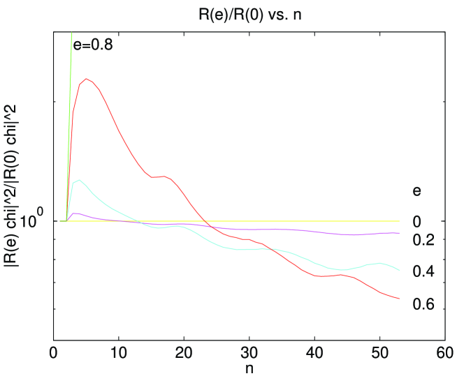
Figure 2: As Fig.1, ratio of remainders for several $e$-values

We see that asymptotically the best inversion is achieved for $e\sim 0.6$ which implies an oblate spectrum. For Monte Carlo application, however, $n\sim 20$ turned out to lead to about optimal results. In this range the value of $e$ is rather uncritical, and $e=0$, where the ellipses degenerate to circles ($e\cosh\theta$ held fixed) and the polynomial to the geometric series, is an acceptable choice. This is also confirmed by some direct Monte Carlo runs. In summary, we found it practical to use inversion as a tool to infer the spectral information necessary to determine the parameters for simulation. The emerging picture was stable for various gauge fields and random $\chi$ that were tested.

Under even-odd preconditioning one replaces $M$ by $\hat{M}=1-M_{\rm oe}M_{\rm eo}$ with $\det M=\det\hat{M}$, and $M_{\rm oe},M_{\rm eo}$ are blocks of $M$ connecting the even/odd sublattices. An application of $\hat{M}$ has the same complexity as $M$, but it is better conditioned. A pair of eigenvalues $\lambda,2-\lambda$ of $M$ is mapped on one eigenvalue of $\hat{M}$ given by their product. Under this mapping ellipses with parameters $d=1,e$ are mapped to ellipses with $\hat{d}=1-e^{2}/2,\hat{e}=e^{2}/2$. In this way the optimal parameters for inversion of $\hat{M}$ are given by the $e$ optimal for $M$. It again turns out, for the lattice parameters of Figs.1,2, that for the $n$ relevant for efficient simulation, $\hat{e}=0$ is close to optimal. The errors for both cases (same degree n) are connected as $|\hat{R}|\sim|R|^{2}$, which implies a much improved approximation for $\hat{M}$. It is interesting that one can prove the relations (for even $n$)

$$\det(\hat{M}-\hat{z}_{k})=\det(M-z_{k^{\prime}})$$ (8)

$$\det(1-\hat{R})={\rm const}\times\det(1-R)$$ (9)

where $k^{\prime}$ is some permutation of $k$. Although $\hat{R}$ is much smaller than $R$, we get (for every single $U$-field) the same weight from the boson fields. As observed in [5] this allows us to stick to $M$ for the boson fields, which yields a much simpler structure for their influence on $U$-updating. Would we use (5) for the acceptance step, then also this would be identical for $R$ or $\hat{R}$. In the stochastic case with (6), however, preconditioning dramatically raises the acceptance such that $n$ may effectively be about halved. This is due to reduced fluctuations in $\hat{R}$ as compared to $R$. It is trivial to derive the inequality

$$\langle q(R,R^{\prime},\chi)\rangle_{\chi}\leq\langle q_{0}(R,R^{\prime})\rangle$$ (10)

and its preconditioned analog. One may thus estimate the loss in acceptance from the noisy method which turned out to be tolerable in the preconditioned data given below (49% down from 75% with $q_{0}$ at $n=8$).

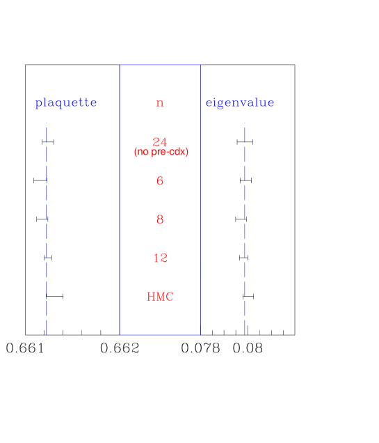
Figure 3: Results for plaquette and lowest eigenvalue of $\hat{M}^{\dagger}\hat{M}$

In Fig.3 results of several multi-boson simulations are shown together with a result from preconditioned HMC for the same parameters[8]. They are obviously completely consistent for a range of acceptances with and without preconditioning. The autocorrelation times are given in the table.

n	pre	acc.(%)	$\tau_{\rm pl}$	$\tau_{\rm ev}$
24	-	88	4.0	21
6	x	27	1.9	3.7
8	x	49	1.3	3.1
12	x	77	1.3	3.9
HMC	x		1.5	1.5

All $\tau$ refer to units of 1000 $M\phi$ applications. The proposals are generated with a certain combination of microcanonical and heatbath sweeps. While the multi-boson algorithm seems advantageous for the plaquette, there is an advantage to HMC for the eigenvalue. In actual CPU time on the Quadrics Q1 the multi-boson algorithm is faster for both quantities for our particular implementations. We plan to clarify this issue further by a simulation on an $8^{4}$ lattice, but it seems likely that without further new ideas there are no large factors in efficiency attainable between the two rather different methods.

I would like to thank Burkhard Bunk for discussions.

References

- [1] M. Lüscher, Nucl. Phys. B418 (1994) 637.
- [2] G. Boyd, B. Alles, M. D’Elia, A. Di Giacomo and E. Vicari, Nucl. Phys. B (Proc.Suppl.) 53 (1997) 544.
- [3] R. Frezzotti and K. Jansen, Phys. Lett. B402 (1997) 328.
- [4] A. Boriçi and P. de Forcrand, Nucl. Phys. B454 (1995) 645.
- [5] A. Borelli, P. de Forcrand and A. Galli, Nucl. Phys. B477 (1996) 809.
- [6] B. Jegerlehner, Nucl. Phys. B (Proc.Suppl.) 53 (1997) 959.
- [7] S. Elser, contribution to this volume.
- [8] K. Jansen, private communication.
- [9] M. Lüscher, R. Sommer, P. Weisz and U. Wolff, Nucl. Phys. B413 (1994) 481.