CPT–97/P.3505

SHEP–97/13

UG–DFM–4/97

hep-lat/9708008

Lattice-Constrained Parametrizations of Form Factors for Semileptonic and Rare Radiative $B$ Decays

UKQCD Collaboration
Luigi Del Debbio¹, Jonathan M Flynn², Laurent Lellouch¹ and Juan Nieves^3
1Centre de Physique Théorique, CNRS Luminy, Case 907 F-13288 Marseille Cedex 9, France

²Department of Physics and Astronomy, University of Southampton, Highfield, Southampton SO17 1BJ, UK

³Departamento de Fisica Moderna, Avenida Fuentenueva, 18071 Granada, Spain

Abstract

We describe all the form factors for semileptonic and radiative $B$ decays to the same light vector meson with just two parameters and the two form factors for semileptonic $B$ decays to a light pseudoscalar meson with a further two or three parameters. This provides simple parametrizations of the form factors for the physical $\bar{B}^{0}\to\rho^{+}l^{-}\bar{\nu}_{l}$, $\bar{B}^{0}\to\pi^{+}l^{-}\bar{\nu}_{l}$ and $\bar{B}\to K^{*}\gamma$ decays. The parametrizations are consistent with heavy quark symmetry, kinematic constraints and lattice results, which we use to determine the parameters. In addition, we test versions of the parametrizations consistent (or not) with light-cone sum rule scaling relations at $q^{2}=0$.

PACS Numbers: 13.20.He, 12.15.Hh, 12.38.Gc, 12.39.Hg

Key-Words: Semileptonic and Rare Radiative Decays of $B$ Mesons, Determination of Cabibbo-Kobayashi-Maskawa Matrix Elements, Lattice QCD Calculation, Heavy Quark Effective Theory.

1 Motivation

The aim of this note is to obtain a simple yet phenomenologically useful description of the form factors for semileptonic and rare radiative heavy-to-light meson decays for all $q^{2}$, the squared four-momentum transfer to the leptons or photon. Lattice calculations provide values for the form factors over a limited region at high $q^{2}$. We supplement these data with further constraints and model input to obtain our parametrization.

The semileptonic decays have been measured by CLEO [1]. Combining those results with our parametrization leads to values for $|V_{ub}|$. The decay $\bar{B}\to K^{*}\gamma$ depends on $|V_{ts}|$ when described in the Standard Model, but since it first occurs at one loop it is an excellent place to search for new physics [2, 3, 4, 5]: in either case it is important to know the relevant form factors.

Kinematic constraints relate some of the form factors at $q^{2}=0$, and light cone sum rule (LCSR) calculations provide further information at low $q^{2}$, particularly on the heavy meson mass dependence of the form factors as that mass becomes large. Specifically, LCSR predict that all the form factors scale like $m_{B}^{-3/2}$ in the $m_{B}\to\infty$ limit. At the other end of the range, near $q^{2}_{\mathrm{max}}$, heavy quark symmetry (HQS) provides, at lowest order, extra relations between the form factors, but (unlike the case of heavy-to-heavy transitions) does not determine the overall normalisation. Extra assumptions are needed to cover the full $q^{2}$ range. For the decays with a light final state vector meson, we apply a simple model due to Stech [6], which uses just two free parameters. For a light final state pseudoscalar we use fits with two or three parameters [7, 8]. The normalisation in each case is determined using lattice data from the UKQCD collaboration [8, 9, 10].

2 Description of Model

In this section, we transcribe the assumptions made by Stech in [6] into the language of HQS. For $q^{2}$ close to $q^{2}_{\mathrm{max}}$, the standard leading order HQS analysis [11, 12] for a $B$ meson decaying semileptonically or radiatively into a light pseudoscalar ($\pi$) or vector ($\mathcal{V}$) meson allows the corresponding matrix elements to be written as:

$$\langle\pi|\bar{q}\gamma^{\mu}b|\bar{B}\rangle=\sqrt{m_{\pi}m_{B}}\mathop{\mathrm{Tr}}\nolimits\left\{\left(\theta_{1}^{\pi}-\frac{{\mathchoice{\c@ncel\displaystyle{p}}{\c@ncel\textstyle{p}}{\c@ncel\scriptstyle{p}}{\c@ncel\scriptscriptstyle{p}}}_{\pi}}{m_{\pi}}\theta_{2}^{\pi}\right)\gamma^{5}\gamma^{\mu}\frac{1+{\mathchoice{\c@ncel\displaystyle{v}}{\c@ncel\textstyle{v}}{\c@ncel\scriptstyle{v}}{\c@ncel\scriptscriptstyle{v}}}}{2}\gamma^{5}\right\}$$ (1)

and

$$\langle\mathcal{V}(\eta)|\bar{q}\Gamma b|\bar{B}\rangle= -i\sqrt{m_{\mathcal{V}}m_{B}}\mathop{\mathrm{Tr}}\nolimits\left\{\left[\left(\theta_{1}^{\mathcal{V}}+\frac{{\mathchoice{\c@ncel\displaystyle{p}}{\c@ncel\textstyle{p}}{\c@ncel\scriptstyle{p}}{\c@ncel\scriptscriptstyle{p}}}_{\mathcal{V}}}{m_{\mathcal{V}}}\theta_{2}^{\mathcal{V}}\right){\mathchoice{\c@ncel\displaystyle{\eta}}{\c@ncel\textstyle{\eta}}{\c@ncel\scriptstyle{\eta}}{\c@ncel\scriptscriptstyle{\eta}}}^{*}\right.\right.$$ (2)

$$+\left.\left.\left(\theta_{3}^{\mathcal{V}}+\frac{{\mathchoice{\c@ncel\displaystyle{p}}{\c@ncel\textstyle{p}}{\c@ncel\scriptstyle{p}}{\c@ncel\scriptscriptstyle{p}}}_{\mathcal{V}}}{m_{\mathcal{V}}}\theta_{4}^{\mathcal{V}}\right)v\cdot\eta^{*}\right]\Gamma\frac{1+{\mathchoice{\c@ncel\displaystyle{v}}{\c@ncel\textstyle{v}}{\c@ncel\scriptstyle{v}}{\c@ncel\scriptscriptstyle{v}}}}{2}\gamma^{5}\right\}\ ,$$

where $v$ is the four-velocity of the $B$ meson, $q$ is the light active quark ($u$ or $s$), and $\Gamma$ denotes either $\gamma^{\mu}(1-\gamma^{5})$ or $q_{\nu}\sigma^{\mu\nu}(1+\gamma^{5})/2$, with $q_{\nu}=(p_{B}-p_{\pi,\mathcal{V}})_{\nu}$. The $\theta_{i}^{\pi,\mathcal{V}}$ are functions of the invariant $v\cdot p_{\pi,\mathcal{V}}$ and are independent of heavy-quark mass and spin, up to ${\mathcal{O}}\left(1/m_{B}\right)$ corrections.

In this language, Stech’s model amounts to considering only the contribution from $\theta_{2}^{\pi,\mathcal{V}}$ and setting all other $\theta$’s to zero. In this sense, the model is a truncation of the HQS results. As we shall see, its usefulness and justification rest on the facts that it satisfies all known constraints and fits the lattice data (available at large $q^{2}$) well. Evaluating the traces in Eqs. (1,2) and solving the resulting equations for the form factors in a standard notation, we find

$$F_{1}(q^{2}) = \sqrt{\frac{m_{B}}{m_{\pi}}}\theta_{2}^{\pi}(v\cdot p_{\pi})$$

$$F_{0}(q^{2}) = \left(1-\frac{q^{2}}{m_{B}^{2}-m^{2}_{\pi}}\right)F_{1}(q^{2})$$

$$A_{0}(q^{2}) = \sqrt{\frac{m_{B}}{m_{\mathcal{V}}}}\theta_{2}^{\mathcal{V}}(v\cdot p_{\mathcal{V}})$$

$$V(q^{2}) = \left(1+\frac{m_{\mathcal{V}}}{m_{B}}\right)A_{0}(q^{2})$$

$$A_{1}(q^{2}) = \frac{m_{B}^{2}+m_{\mathcal{V}}^{2}}{m_{B}(m_{B}+m_{\mathcal{V}})}\left(1-\frac{q^{2}}{m_{B}^{2}+m_{\mathcal{V}}^{2}}\right)A_{0}(q^{2})$$

$$A_{2}(q^{2}) = \frac{m_{B}+m_{\mathcal{V}}}{m_{B}}\left(1-\frac{2m_{\mathcal{V}}(m_{B}+m_{\mathcal{V}})}{(m_{B}+m_{\mathcal{V}})^{2}-q^{2}}\right)A_{0}(q^{2})$$

$$2T_{1}(q^{2}) = A_{0}(q^{2})$$

$$2iT_{2}(q^{2}) = \left(1-\frac{q^{2}}{m_{B}^{2}-m_{\mathcal{V}}^{2}}\right)A_{0}(q^{2})\ ,$$ (3)

which are equivalent to the relations given in Eq.(11) of Ref. [6] with, in addition, relations involving $T_{1}$ and $T_{2}$.

As we will see below, these relations can be used for a simple and successful description of lattice results for the form factors. We recall that, by construction, this model respects HQS scaling relations and satisfies the two kinematic constraints:

$$F_{1}(0)=F_{0}(0),\qquad T_{1}(0)=iT_{2}(0)$$ (4)

For the parametrization to be complete we must specify the functions $\theta_{2}^{\pi,\mathcal{V}}$. This will be discussed in Section 4.

3 Lattice Details

The details of the lattice simulation can be found in Ref. [8]. The chiral extrapolations for $\bar{B}^{0}\to\rho^{+}l^{-}\bar{\nu}_{l}$ and $\bar{B}\to K^{*}\gamma$ are described in Ref. [9] while those for $\bar{B}^{0}\to\pi^{+}l^{-}\bar{\nu}_{l}$ are explained in Ref. [7]. The only way in which our determination of the lattice form factors differs here is in the heavy-quark mass extrapolation. We improve this extrapolation for the form factors $A_{1}$, $V$, $T_{1}$ and $T_{2}$ by imposing heavy quark symmetry in the infinite heavy-quark mass limit, as we now explain.

All form factors are calculated for four values of the heavy quark mass around the charm mass and for a variety of values of $q^{2}$. In previous work [8, 9], the form factors were extrapolated at fixed four-velocity recoil, $\omega=v\cdot(p_{\pi,\mathcal{V}}/m_{\pi,\mathcal{V}})$, near the zero recoil point $\omega=1$, by fitting to the following heavy-quark scaling relations:

$$f\Theta M^{N_{f}/2}=\gamma_{f}(1+\frac{\delta_{f}}{M}+\frac{\epsilon_{f}}{M^{2}}+\cdots)$$ (5)

where $f=F_{1},F_{0},A_{0},V,A_{1},A_{2},T_{1},T_{2}$ and $N_{f}=-1,1,-1,-1,1,-1,-1,1$ respectively. Here, $M$ is the mass of the heavy-light meson, $\gamma_{f}$, $\delta_{f}$ and $\epsilon_{f}$ are the fit parameters, and $\Theta$ comes from leading logarithmic matching and is chosen to be 1 at the $B$ mass [13],

$$\Theta=\Theta(M/m_{B})=\left(\frac{\alpha_{s}(M)}{\alpha_{s}(m_{B})}\right)^{\frac{2}{\beta_{0}}},$$ (6)

with $\beta_{0}=11$ in the quenched approximation and $\Lambda_{\rm QCD}=200\,\mathrm{Me\kern-1.00006ptV}$.

While correct, this procedure neglects the fact that in the $M\to\infty$ limit, HQS predicts

$$A_{1}(q^{2})=2iT_{2}(q^{2}),\quad V(q^{2})=2T_{1}(q^{2})$$ (7)

for $q^{2}$ not too far from $q^{2}_{\mathrm{max}}$, i.e. close to zero recoil. In the present paper, we enforce this prediction of HQS by performing a combined fit, at fixed $\omega$, of the pairs of form factors $(A_{1},T_{2})$ and $(V,T_{1})$ to the parametrizations of Eq. (5) with the following constraints on the fit parameters:

$$\gamma_{A_{1}}=2i\gamma_{T_{2}},\quad\gamma_{V}=2\gamma_{T_{1}}\ .$$ (8)

This not only guarantees that the extrapolated form factors are consistent with HQS in the infinite mass limit, but also reduces statistical errors, because the number of parameters is decreased.

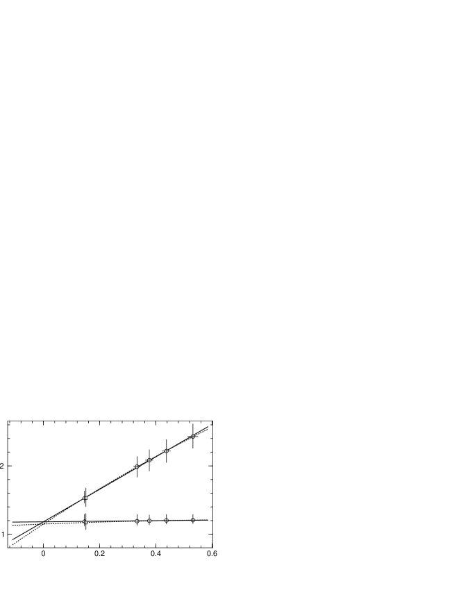
$V\sqrt{m_{B}/M}\mathrm{\ or\ }2T_{1}\sqrt{m_{B}/M}$ $0\to 1\mathrm{\ channel,\ }\omega=1.34(2)$ $m_{\rho}/M$

Figure 1: Constrained $1/M$ extrapolation of the pair of form factors $(V,2T_{1})$, as described in the text. The solid curves correspond to a linear extrapolation, the dashed curves to a quadratic fit. The four lower circle points are the lattice results for $2T_{1}\sqrt{m_{B}/M}$ and the four upper ones are those for $V\sqrt{m_{B}/M}$, in the case where a $B$ meson at rest decays to produce a $\rho$ meson with one (lattice) unit of three momentum. The points at $m_{\rho}/M=0.146$ correspond to the linearly (diamonds) and quadratically (squares) extrapolated results for the two form factors at $M=m_{B}$.

As an example, we show in Fig. 1 the combined fit of $(V,2T_{1})$ to the constrained heavy quark scaling relation just described, for the case of a final state $\rho$. Both the linear and quadratic fits in $1/M$ are excellent, confirming our earlier finding, in Ref. [9], that the form factors $A_{1}$, $V$, $T_{1}$ and $T_{2}$ satisfy the infinite mass relations of Eq. (7) very well, even when extrapolated independently. Because linear and quadratic extrapolations always give results which agree within error, because the quadratic term is always consistent with 0 and because the quadratic fits may emphasize small discretization errors, we will use the linear results in the following.

In the results reported below, all errors are statistical central 68% bounds. For decays to a light final state vector we use 250 bootstrap samples from our lattice data. For decays to a light pseudoscalar we add errors to account for the chiral extrapolation [7] and propagate them assuming standard Gaussian statistics.

4 Form Factors

One could imagine performing a combined fit to $\bar{B}^{0}\to\pi^{+}l^{-}\bar{\nu}_{l}$, $\bar{B}^{0}\to\rho^{+}l^{-}\bar{\nu}_{l}$ and $\bar{B}\to K^{*}\gamma$ form factors assuming $\theta_{2}^{\pi}(q^{2}){=}\theta_{2}^{\mathcal{V}}(q^{2})$ in Eq. (3). However, there is no reason to have spin symmetry relating the final pseudoscalar and vector states. Furthermore, our lattice results clearly indicate that the $q^{2}$ dependences of $F_{1}(q^{2})$ and $A_{0}(q^{2})$ are different, in contradiction to the assumption $\theta_{2}^{\pi}(q^{2})=\theta_{2}^{\mathcal{V}}(q^{2})$. Thus we consider decays to pseudoscalar and vector states separately.

4.1 $\bar{B}^{0}\to\rho^{+}l^{-}\bar{\nu}_{l}$ and $\bar{B}\to K^{*}\gamma$ decays

So as not to assume flavour $SU(3)$ symmetry in our combined description of $\bar{B}^{0}\to\rho^{+}l^{-}\bar{\nu}_{l}$ and $\bar{B}\to K^{*}\gamma$ decays we have used the freedom to adjust quark masses in lattice calculations and considered two situations:

• The mass of the light active quark $q$ in Eq. (2) is set to the $u$ quark mass (i.e. $\mathcal{V}=\rho$ in Eqs. (2,3)). In this case, the combined fit to the form factors of the operators $\bar{q}\gamma^{\mu}(1{-}\gamma^{5})b$ and $\bar{q}q_{\nu}\sigma^{\mu\nu}(1{+}\gamma^{5})b/2$ constrains, through Eq. (3), the form factors relevant for the decay $\bar{B}^{0}\to\rho^{+}l^{-}\bar{\nu}_{l}$.

• The mass of the light active quark $q$ in Eq. (2) is set to the $s$ quark mass (i.e. $\mathcal{V}=K^{*}$ in Eqs. (2,3)). Now the combined fit constrains, through Eq. (3), the form factors relevant for the decay $\bar{B}\to K^{*}\gamma$.

For the parametrization of Eq. (3) to be complete we must specify the function $\theta_{2}^{\mathcal{V}}$ or, equivalently, one of the form factors. With pole dominance ideas in mind, we shall consider a pole form for $A_{1}(q^{2})$ which is compatible with previous lattice analyses [9] and LCSR results [14]:

$$A_{1}(q^{2})=\frac{A_{1}(0)}{1-q^{2}/M_{1}^{2}}\ ,$$ (9)

where the two free parameters are $A_{1}(0)$ and $M_{1}$, a mass on the order of $m_{B}$. With these two parameters alone, we can describe the six form factors needed for decays to a vector final state. This form further guarantees that all form factors scale like $m_{B}^{-3/2}$ at $q^{2}=0$ as predicted by LCSR in Ref. [14]. The results for $\bar{B}^{0}\to\rho^{+}l^{-}\bar{\nu}_{l}$ and $\bar{B}\to K^{*}\gamma$ decays are presented in Tab. 1, and Figs. 2 and 3. As the $\chi^{2}$ indicates, this simple parametrization works surprisingly well. The $SU(3)$ flavour dependence in our results, from comparing situations A and B, is mild. Corresponding form factor values at $q^{2}=0$ differ by less than 10%.

$\bar{B}^{0}\to\rho^{+}l^{-}\bar{\nu}_{l}$ $A_{1}(0)=0.27{{\mathop{\raisebox{0.1pt}{\scriptsize$\begin{array}[]{@{}c@{}}+\\ -\end{array}$}}\raisebox{0.1pt}{\scriptsize$\begin{array}[]{@{}r@{}}0.05\\ 0.04\end{array}$}}}$ $M_{1}=7.0{{\mathop{\raisebox{0.1pt}{\scriptsize$\begin{array}[]{@{}c@{}}+\\ -\end{array}$}}\raisebox{0.1pt}{\scriptsize$\begin{array}[]{@{}r@{}}1.2\\ 0.6\end{array}$}}}\,\mathrm{Ge\kern-1.00006ptV}$ $\chi^{2}/\mathrm{dof}=24/20$ $A_{1}$ $A_{2}$ $A_{0}$ $V$ $q^{2}{=}0$ $0.27{{\mathop{\raisebox{0.1pt}{\scriptsize$\begin{array}[]{@{}c@{}}+\\ -\end{array}$}}\raisebox{0.1pt}{\scriptsize$\begin{array}[]{@{}r@{}}0.05\\ 0.04\end{array}$}}}$ $0.26{{\mathop{\raisebox{0.1pt}{\scriptsize$\begin{array}[]{@{}c@{}}+\\ -\end{array}$}}\raisebox{0.1pt}{\scriptsize$\begin{array}[]{@{}r@{}}0.05\\ 0.03\end{array}$}}}$ $0.30{{\mathop{\raisebox{0.1pt}{\scriptsize$\begin{array}[]{@{}c@{}}+\\ -\end{array}$}}\raisebox{0.1pt}{\scriptsize$\begin{array}[]{@{}r@{}}0.06\\ 0.04\end{array}$}}}$ $0.35{{\mathop{\raisebox{0.1pt}{\scriptsize$\begin{array}[]{@{}c@{}}+\\ -\end{array}$}}\raisebox{0.1pt}{\scriptsize$\begin{array}[]{@{}r@{}}0.06\\ 0.05\end{array}$}}}$ $q^{2}_{\mathrm{max}}$ $0.46{{\mathop{\raisebox{0.1pt}{\scriptsize$\begin{array}[]{@{}c@{}}+\\ -\end{array}$}}\raisebox{0.1pt}{\scriptsize$\begin{array}[]{@{}r@{}}0.02\\ 0.01\end{array}$}}}$ $0.88{{\mathop{\raisebox{0.1pt}{\scriptsize$\begin{array}[]{@{}c@{}}+\\ -\end{array}$}}\raisebox{0.1pt}{\scriptsize$\begin{array}[]{@{}r@{}}0.05\\ 0.03\end{array}$}}}$ $1.80{{\mathop{\raisebox{0.1pt}{\scriptsize$\begin{array}[]{@{}c@{}}+\\ -\end{array}$}}\raisebox{0.1pt}{\scriptsize$\begin{array}[]{@{}r@{}}0.09\\ 0.05\end{array}$}}}$ $2.07{{\mathop{\raisebox{0.1pt}{\scriptsize$\begin{array}[]{@{}c@{}}+\\ -\end{array}$}}\raisebox{0.1pt}{\scriptsize$\begin{array}[]{@{}r@{}}0.11\\ 0.06\end{array}$}}}$ $\bar{B}\to K^{*}\gamma$ $A_{1}(0)=0.29{{\mathop{\raisebox{0.1pt}{\scriptsize$\begin{array}[]{@{}c@{}}+\\ -\end{array}$}}\raisebox{0.1pt}{\scriptsize$\begin{array}[]{@{}r@{}}0.04\\ 0.03\end{array}$}}}$ $M_{1}=6.8{{\mathop{\raisebox{0.1pt}{\scriptsize$\begin{array}[]{@{}c@{}}+\\ -\end{array}$}}\raisebox{0.1pt}{\scriptsize$\begin{array}[]{@{}r@{}}0.7\\ 0.4\end{array}$}}}\,\mathrm{Ge\kern-1.00006ptV}$ $\chi^{2}/\mathrm{dof}=27/20$ $T_{1}$ $T_{2}$ $q^{2}{=}0$ $0.16{{\mathop{\raisebox{0.1pt}{\scriptsize$\begin{array}[]{@{}c@{}}+\\ -\end{array}$}}\raisebox{0.1pt}{\scriptsize$\begin{array}[]{@{}r@{}}0.02\\ 0.01\end{array}$}}}$ $q^{2}_{\mathrm{max}}$ $0.90{{\mathop{\raisebox{0.1pt}{\scriptsize$\begin{array}[]{@{}c@{}}+\\ -\end{array}$}}\raisebox{0.1pt}{\scriptsize$\begin{array}[]{@{}r@{}}0.05\\ 0.04\end{array}$}}}$ $0.25{{\mathop{\raisebox{0.1pt}{\scriptsize$\begin{array}[]{@{}c@{}}+\\ -\end{array}$}}\raisebox{0.1pt}{\scriptsize$\begin{array}[]{@{}r@{}}0.01\\ 0.01\end{array}$}}}$

Table 1: Results of fits to the lattice predictions for $A_{0}$, $A_{1}$, $V$, $T_{1}$ and $T_{2}$ assuming a pole form for $A_{1}$, as given in Eq. (9), in the parametrization of Eq. (3). On the left are results for a $\rho$ meson final state (Situation A) and on the right, results for a $K^{*}$ meson final state (Situation B). We also provide the values of the form factors for $\bar{B}^{0}\to\rho^{+}l^{-}\bar{\nu}_{l}$ and $\bar{B}\to K^{*}\gamma$ decays at $q^{2}{=}0$ and $q^{2}_{\mathrm{max}}$, as determined by the fit.

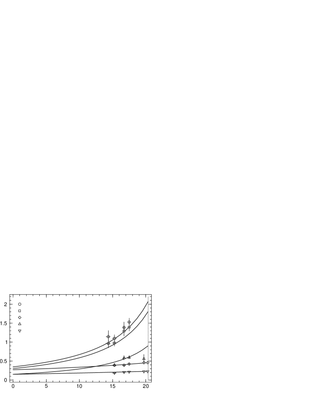
$V$ $A_{0}$ $A_{1}$ $T_{1}$ $T_{2}$ $q^{2}\;(\,\mathrm{Ge\kern-1.00006ptV}^{2})$

Figure 2: Fit to the lattice predictions for $A_{0}$, $A_{1}$, $V$, $T_{1}$ and $T_{2}$ for a $\rho$ meson final state (Situation A) using the parametrization of Eq. (3) and assuming a pole form for $A_{1}$ as given in Eq. (9). The dashed vertical line indicates $q^{2}_{\mathrm{max}}$.

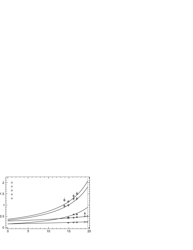
$V$ $A_{0}$ $A_{1}$ $T_{1}$ $T_{2}$ $q^{2}(\,\mathrm{Ge\kern-1.00006ptV}^{2})$

Figure 3: Fit to the lattice predictions for $A_{0}$, $A_{1}$, $V$, $T_{1}$ and $T_{2}$ for a $K^{*}$ meson final state (Situation B) using the parametrization of Eq. (3) and assuming a pole form for $A_{1}$ as given in Eq. (9). The dashed vertical line indicates $q^{2}_{\mathrm{max}}$.

We have considered functional dependences for $A_{1}$ different from that in Eq. (9). Constant behaviour has already been ruled out by lattice results Ref. [9]. Dipole (and in general higher powers: tripole, …) and pole fits are hardly distinguishable in the physical range $0\leq q^{2}\leq q^{2}_{\mathrm{max}}$. In a dipole fit, the mass parameter $M_{\rm dipole}$ is roughly given by $M_{\rm dipole}\approx\sqrt{2}M_{\rm pole}$ and hence pole and dipole fits agree in the range of values of $q^{2}$ explored in Figs. 2 and 3. We have also studied “modified-constant” behaviour for $A_{1}$:

$$A_{1}(q^{2})=(1-q^{2}/m_{\alpha}^{2})\frac{A_{1}(0)}{1-q^{2}/m_{\beta}^{2}}\ ,$$ (10)

where $m_{\alpha}$ and $m_{\beta}$ are masses on the order of $m_{B}$. Such a behaviour was introduced in Ref. [7] in the context of $B\to\pi l\nu$ decays. Within the framework of Eq. (3), this can be implemented by parametrizing $A_{0}(q^{2})$ as a pole without increasing the number of free parameters. Thus, we have performed a second set of fits where we complete the parametrization of Eq. (3) by taking the following functional form for $A_{0}$:

$$A_{0}(q^{2})=\frac{A_{0}(0)}{1-q^{2}/M_{0}^{2}}$$ (11)

where the two free parameters are $A_{0}(0)$ and $M_{0}$, a mass of the order of $m_{B}$. The corresponding results for $\bar{B}^{0}\to\rho^{+}l^{-}\bar{\nu}_{l}$ and $\bar{B}\to K^{*}\gamma$ decays are presented in Tab. 2. This parametrization yields different behaviour for the form factors at small $q^{2}$: the values at $q^{2}=0$ differ by two to three standard deviations.

$\bar{B}^{0}\to\rho^{+}l^{-}\bar{\nu}_{l}$ $A_{0}(0)=0.40{{\mathop{\raisebox{0.1pt}{\scriptsize$\begin{array}[]{@{}c@{}}+\\ -\end{array}$}}\raisebox{0.1pt}{\scriptsize$\begin{array}[]{@{}r@{}}0.04\\ 0.03\end{array}$}}}$ $M_{0}=5.10{{\mathop{\raisebox{0.1pt}{\scriptsize$\begin{array}[]{@{}c@{}}+\\ -\end{array}$}}\raisebox{0.1pt}{\scriptsize$\begin{array}[]{@{}r@{}}0.08\\ 0.06\end{array}$}}}\,\mathrm{Ge\kern-1.00006ptV}$ $\chi^{2}/\mathrm{dof}=25/20$ $A_{1}$ $A_{2}$ $A_{0}$ $V$ $q^{2}{=}0$ $0.35{{\mathop{\raisebox{0.1pt}{\scriptsize$\begin{array}[]{@{}c@{}}+\\ -\end{array}$}}\raisebox{0.1pt}{\scriptsize$\begin{array}[]{@{}r@{}}0.03\\ 0.02\end{array}$}}}$ $0.34{{\mathop{\raisebox{0.1pt}{\scriptsize$\begin{array}[]{@{}c@{}}+\\ -\end{array}$}}\raisebox{0.1pt}{\scriptsize$\begin{array}[]{@{}r@{}}0.03\\ 0.02\end{array}$}}}$ $0.40{{\mathop{\raisebox{0.1pt}{\scriptsize$\begin{array}[]{@{}c@{}}+\\ -\end{array}$}}\raisebox{0.1pt}{\scriptsize$\begin{array}[]{@{}r@{}}0.04\\ 0.03\end{array}$}}}$ $0.45{{\mathop{\raisebox{0.1pt}{\scriptsize$\begin{array}[]{@{}c@{}}+\\ -\end{array}$}}\raisebox{0.1pt}{\scriptsize$\begin{array}[]{@{}r@{}}0.04\\ 0.03\end{array}$}}}$ $q^{2}_{\mathrm{max}}$ $0.46{{\mathop{\raisebox{0.1pt}{\scriptsize$\begin{array}[]{@{}c@{}}+\\ -\end{array}$}}\raisebox{0.1pt}{\scriptsize$\begin{array}[]{@{}r@{}}0.02\\ 0.01\end{array}$}}}$ $0.89{{\mathop{\raisebox{0.1pt}{\scriptsize$\begin{array}[]{@{}c@{}}+\\ -\end{array}$}}\raisebox{0.1pt}{\scriptsize$\begin{array}[]{@{}r@{}}0.05\\ 0.03\end{array}$}}}$ $1.81{{\mathop{\raisebox{0.1pt}{\scriptsize$\begin{array}[]{@{}c@{}}+\\ -\end{array}$}}\raisebox{0.1pt}{\scriptsize$\begin{array}[]{@{}r@{}}0.10\\ 0.06\end{array}$}}}$ $2.08{{\mathop{\raisebox{0.1pt}{\scriptsize$\begin{array}[]{@{}c@{}}+\\ -\end{array}$}}\raisebox{0.1pt}{\scriptsize$\begin{array}[]{@{}r@{}}0.11\\ 0.06\end{array}$}}}$ $\bar{B}\to K^{*}\gamma$ $A_{0}(0)=0.42{{\mathop{\raisebox{0.1pt}{\scriptsize$\begin{array}[]{@{}c@{}}+\\ -\end{array}$}}\raisebox{0.1pt}{\scriptsize$\begin{array}[]{@{}r@{}}0.03\\ 0.02\end{array}$}}}$ $M_{0}=5.05{{\mathop{\raisebox{0.1pt}{\scriptsize$\begin{array}[]{@{}c@{}}+\\ -\end{array}$}}\raisebox{0.1pt}{\scriptsize$\begin{array}[]{@{}r@{}}0.06\\ 0.05\end{array}$}}}\,\mathrm{Ge\kern-1.00006ptV}$ $\chi^{2}/\mathrm{dof}=27/20$ $T_{1}$ $T_{2}$ $q^{2}{=}0$ $0.21{{\mathop{\raisebox{0.1pt}{\scriptsize$\begin{array}[]{@{}c@{}}+\\ -\end{array}$}}\raisebox{0.1pt}{\scriptsize$\begin{array}[]{@{}r@{}}0.01\\ 0.01\end{array}$}}}$ $q^{2}_{\mathrm{max}}$ $0.91{{\mathop{\raisebox{0.1pt}{\scriptsize$\begin{array}[]{@{}c@{}}+\\ -\end{array}$}}\raisebox{0.1pt}{\scriptsize$\begin{array}[]{@{}r@{}}0.05\\ 0.04\end{array}$}}}$ $0.25{{\mathop{\raisebox{0.1pt}{\scriptsize$\begin{array}[]{@{}c@{}}+\\ -\end{array}$}}\raisebox{0.1pt}{\scriptsize$\begin{array}[]{@{}r@{}}0.01\\ 0.01\end{array}$}}}$

Table 2: Results of fits to the lattice predictions for $A_{0}$, $A_{1}$, $V$, $T_{1}$ and $T_{2}$ assuming a pole form for $A_{0}$, as given in Eq. (11), in the parametrization of Eq. (3). On the left are results for a $\rho$ meson final state (Situation A) and on the right, results for a $K^{*}$ meson final state (Situation B). We also provide the values of the form factors relevant for $\bar{B}^{0}\to\rho^{+}l^{-}\bar{\nu}_{l}$ and $\bar{B}\to K^{*}\gamma$ decays at $q^{2}{=}0$ and $q^{2}_{\mathrm{max}}$ as determined by the fit.

Though we cannot discriminate against this parametrization on the basis of $\chi^{2}$ alone, there are physical arguments for preferring the $A_{1}$ pole fits. Fixing pole behaviour for $A_{0}$ in the context of Stech’s parametrization forces all form factors to diverge at the same value of $q^{2}$ even though different form factors receive contributions from resonances with different quantum numbers and masses. Furthermore, we find that this divergence occurs at around $5.1\,\mathrm{Ge\kern-1.00006ptV}$, below the first physical pole, the $B$. Assuming pole behaviour for $A_{1}$, on the other hand, allows the form factors which receive contributions from $1^{+}$ resonances ($A_{1}$, $A_{2}$ and $T_{2}$) to diverge at larger values of $q^{2}$ than the more singular form factors $V$, $T_{1}$ and $A_{0}$. Our fit confirms such behaviour as we find $M_{1}=7.0{{\mathop{\raisebox{0.1pt}{\scriptsize$\begin{array}[]{@{}c@{}}+\\ -\end{array}$}}\raisebox{0.1pt}{\scriptsize$\begin{array}[]{@{}r@{}}1.2\\ 0.6\end{array}$}}}\,\mathrm{Ge\kern-1.00006ptV}$, in reasonable agreement with lattice [15] and quark model estimates [16, 17, 18] for the $1^{+}$, $b\bar{q}$ resonance. The more singular form factors then diverge at $q^{2}=m_{B}^{2}+m_{\mathcal{V}}^{2}$ which is close to the physical $0^{-}$ ($A_{0}$) and $1^{-}$ ($V$ and $T_{1}$) poles. Finally, LCSR scaling relations at $q^{2}=0$ combined with HQS requirements at $q^{2}_{\mathrm{max}}$ rule out pole behaviour for $A_{0}$ but not for $A_{1}$. Thus, for physical applications, we consider only the parametrization given in Eqs. (3,9).

4.2 $\bar{B}^{0}\to\pi^{+}l^{-}\bar{\nu}_{l}$ decays

Stech’s parametrization predicts that $F_{0}(q^{2}_{\mathrm{max}})$ vanishes in the chiral limit, in contradiction with our results and made unlikely by unitarity bounds [7]. Furthermore, the $B^{*}$ which contributes a pole to $F_{1}$ induces the same singularity in $F_{0}$ within Stech’s model. Because the $B^{*}$ pole is very close to $q^{2}_{\mathrm{max}}$, it provokes a much more pronounced $q^{2}$ dependence for $F_{0}$ than observed in the lattice results or induced by the nearest resonance in this $0^{+}$ channel whose mass is significantly larger than $m_{B^{*}}$.

Restricting to polar-type $q^{2}$-dependences, consistent with the kinematical constraint, $F_{1}(0)=F_{0}(0)$, heavy quark symmetry and unitarity bounds [7, 8], we consider two possible functional forms:

• pole/dipole

  $$F_{1}(q^{2})=\frac{F(0)}{\left(1-q^{2}/m_{1}^{2}\right)^{2}}\,,\qquad F_{0}(q^{2})=\frac{F(0)}{\left(1-q^{2}/m_{0}^{2}\right)}$$ (12)

• “modified-constant”/pole

  $$F_{1}(q^{2})=\frac{F(0)}{\left(1-q^{2}/m_{1}^{2}\right)}\,,\qquad F_{0}(q^{2})=F(0)\frac{(1-q^{2}/m_{2}^{2})}{\left(1-q^{2}/m_{0}^{2}\right)}$$ (13)

These two dependences have been studied previously in Ref. [8] with light quark masses slightly larger than that of the strange quark and in Ref. [7] for massless $u$ and $d$ quarks. The fit results are summarized here in Tab. 3. We note that only the pole-dipole parametrization is consistent with LCSR scaling relations at $q^{2}=0$ together with HQS requirements at $q^{2}_{\mathrm{max}}$. Both fits are consistent with the dispersive bounds of Ref. [7].

fit type	$F(0)$	$m_{1}\,(\,\mathrm{Ge\kern-1.00006ptV})$	$m_{0}\,(\,\mathrm{Ge\kern-1.00006ptV})$	$m_{2}\,(\,\mathrm{Ge\kern-1.00006ptV})$	$\chi^{2}/\mathrm{dof}$
“modified-const”	$0.43\pm 0.06$	$m_{B^{*}}$	5.5	$5.89\pm 0.52$	0.5/4
pole/dipole	$0.27\pm 0.11$	$5.79\pm 0.58$	$6.1\pm 1.5$	–	0.1/3

Table 3: Fits of the lattice results for $F_{1}(q^{2})$ and $F_{0}(q^{2})$ to the parametrizations described in the text (taken from Ref. [7]). In order to perform the “modified-constant/pole” fit with a limited range of results, $m_{1}$ and $m_{0}$ were fixed to the value of the corresponding nearest resonances. (This latter fit is named “fixed-pole” in Ref. [7].)

5 Phenomenological Consequences

Using the preferred pole form for $A_{1}$ in the decay $\bar{B}^{0}\to\rho^{+}l^{-}\bar{\nu}_{l}$, we find the differential decay rate spectra in $q^{2}$ and the lepton energy $E$. These are shown in Fig. 4. Likewise, using the pole/dipole fits for $\bar{B}^{0}\to\pi^{+}l^{-}\bar{\nu}_{l}$, we find the differential spectra shown in Fig. 5. Integrating to find the total decay rates we have, for massless leptons in the final state:

$$\Gamma(\bar{B}^{0}\to\rho^{+}l^{-}\bar{\nu}_{l})/|V_{ub}|^{2} = 10.9{{\mathop{\raisebox{0.1pt}{\scriptsize$\begin{array}[]{@{}c@{}}+\\ -\end{array}$}}\raisebox{0.1pt}{\scriptsize$\begin{array}[]{@{}r@{}}2.3\\ 1.5\end{array}$}}}\times 10^{-12}\,\mathrm{Ge\kern-1.00006ptV}=16.5{{\mathop{\raisebox{0.1pt}{\scriptsize$\begin{array}[]{@{}c@{}}+\\ -\end{array}$}}\raisebox{0.1pt}{\scriptsize$\begin{array}[]{@{}r@{}}3.5\\ 2.3\end{array}$}}}\,\mathrm{ps}^{-1}$$ (22)

$$\Gamma(\bar{B}^{0}\to\pi^{+}l^{-}\bar{\nu}_{l})/|V_{ub}|^{2} = 5.6{{\mathop{\raisebox{0.1pt}{\scriptsize$\begin{array}[]{@{}c@{}}+\\ -\end{array}$}}\raisebox{0.1pt}{\scriptsize$\begin{array}[]{@{}r@{}}2.2\\ 0.6\end{array}$}}}\times 10^{-12}\,\mathrm{Ge\kern-1.00006ptV}=8.5{{\mathop{\raisebox{0.1pt}{\scriptsize$\begin{array}[]{@{}c@{}}+\\ -\end{array}$}}\raisebox{0.1pt}{\scriptsize$\begin{array}[]{@{}r@{}}3.4\\ 0.9\end{array}$}}}\,\mathrm{ps}^{-1}$$ (31)

For decays with a tau lepton in the final state we find:

$$\Gamma(\bar{B}^{0}\to\rho^{+}\tau^{-}\bar{\nu}_{\tau})/|V_{ub}|^{2} = 5.8{{\mathop{\raisebox{0.1pt}{\scriptsize$\begin{array}[]{@{}c@{}}+\\ -\end{array}$}}\raisebox{0.1pt}{\scriptsize$\begin{array}[]{@{}r@{}}0.9\\ 0.6\end{array}$}}}\times 10^{-12}\,\mathrm{Ge\kern-1.00006ptV}=8.8{{\mathop{\raisebox{0.1pt}{\scriptsize$\begin{array}[]{@{}c@{}}+\\ -\end{array}$}}\raisebox{0.1pt}{\scriptsize$\begin{array}[]{@{}r@{}}1.4\\ 0.9\end{array}$}}}\,\mathrm{ps}^{-1}$$ (40)

$$\Gamma(\bar{B}^{0}\to\pi^{+}\tau^{-}\bar{\nu}_{\tau})/|V_{ub}|^{2} = 3.8{{\mathop{\raisebox{0.1pt}{\scriptsize$\begin{array}[]{@{}c@{}}+\\ -\end{array}$}}\raisebox{0.1pt}{\scriptsize$\begin{array}[]{@{}r@{}}1.2\\ 0.2\end{array}$}}}\times 10^{-12}\,\mathrm{Ge\kern-1.00006ptV}=5.8{{\mathop{\raisebox{0.1pt}{\scriptsize$\begin{array}[]{@{}c@{}}+\\ -\end{array}$}}\raisebox{0.1pt}{\scriptsize$\begin{array}[]{@{}r@{}}1.8\\ 0.4\end{array}$}}}\,\mathrm{ps}^{-1}$$ (49)

$d\Gamma/dq^{2}\;(|V_{ub}|^{2}10^{-12}\,\mathrm{Ge\kern-1.00006ptV}^{-1})$ $d\Gamma/dE\;(|V_{ub}|^{2}10^{-12})$ $q^{2}(\,\mathrm{Ge\kern-1.00006ptV}^{2})$ $E(\,\mathrm{Ge\kern-1.00006ptV})$

Figure 4: Differential decay spectra for $\bar{B}^{0}\to\rho^{+}l^{-}\bar{\nu}_{l}$ for massless leptons: (a) $d\Gamma/dq^{2}$ in units of $10^{-12}|V_{ub}|^{2}\,\mathrm{Ge\kern-1.00006ptV}^{-1}$, (b) $d\Gamma/dE$ in units of $10^{-12}|V_{ub}|^{2}$. The form factors are taken from the fit to the parametrization of Eq. (3), assuming a pole form for $A_{1}$ as given in Eq. (9). The dashed lines show the envelope of the 68% bootstrap errors computed separately for each value of $q^{2}$ or $E$ respectively.

$d\Gamma/dq^{2}\;(|V_{ub}|^{2}10^{-12}\,\mathrm{Ge\kern-1.00006ptV}^{-1})$ $d\Gamma/dE\;(|V_{ub}|^{2}10^{-12})$ $q^{2}(\,\mathrm{Ge\kern-1.00006ptV}^{2})$ $E(\,\mathrm{Ge\kern-1.00006ptV})$

Figure 5: Differential decay spectra for $\bar{B}^{0}\to\pi^{+}l^{-}\bar{\nu}_{l}$ for massless leptons: (a) $d\Gamma/dq^{2}$ in units of $10^{-12}|V_{ub}|^{2}\,\mathrm{Ge\kern-1.00006ptV}^{-1}$, (b) $d\Gamma/dE$ in units of $10^{-12}|V_{ub}|^{2}$. The form factors are taken from the fit with a dipole form for $F_{1}$ as given in Eq. (12). The dashed lines show the envelope of the 68% errors computed separately for each value of $q^{2}$ or $E$ respectively.

In Tab. 4 we compare our results with recent LCSR [14, 20, 21, 22, 23, 24] calculations. The agreement of the form factor values at $q^{2}=0$ is very good. In the spectrum $d\Gamma(\bar{B}^{0}\to\rho^{+}l^{-}\bar{\nu}_{l})/dq^{2}$ we note that our result is larger near $q^{2}=0$, as is our value for the ratio $\Gamma_{L}/\Gamma_{T}$. The differential decay rate at $q^{2}=0$ is proportional to

$$A_{0}(0)={m_{B}+m_{\rho}\over 2m_{\rho}}A_{1}(0)-{m_{B}-m_{\rho}\over 2m_{\rho}}A_{2}(0)\ ,$$ (50)

which is the longitudinal contribution, so that small differences in $A_{1}(0)$ and $A_{2}(0)$ can lead to significant differences in the differential rate and in the ratio of longitudinal to transverse rates. Since the lattice results are available for large $q^{2}$, the $d\Gamma/dq^{2}$ plots in Figs. 4 and 5 also show errors growing larger towards $q^{2}=0$. This is complementary behaviour to LCSR results, which are more reliable at low $q^{2}$.

All other rates agree with the LCSR results within errors. Agreement is also excellent with the experimental results of CLEO [1]. For the ratio $\Gamma(\rho)/\Gamma(\pi)$, which is independent of $|V_{ub}|$ and can therefore be compared directly to the value in Tab. 4, CLEO quotes $1.4{{\mathop{\raisebox{0.1pt}{\scriptsize$\begin{array}[]{@{}c@{}}+\\ -\end{array}$}}\raisebox{0.1pt}{\scriptsize$\begin{array}[]{@{}r@{}}0.6\\ 0.4\end{array}$}}}\pm 0.3\pm 0.4$, where the errors are statistical, systematic and the estimated model dependence. Moreover, branching ratios, obtained from the rates in Tab. 4 with the values of $|V_{ub}|$ and of the $B$ lifetimes given in Ref. [1] by CLEO, compare very favorably with the values in that same publication.

Finally, the additional constraints provided by our approach may shed some light on the twofold ambiguity in the lattice value of $T_{1}(0)$ (see for example [8, 26]) by favouring the smaller of the two determinations. With our prediction for $T_{1}(0)$, we can determine the hadronization ratio $R_{K^{*}}=\Gamma(B\to K^{*}\gamma)/\Gamma(b\to s\gamma)$, which is given, up to ${\mathcal{O}}\left(1/m_{b}^{2}\right)$ corrections, by [27]

$$R_{K^{*}}=4\left(\frac{m_{B}}{m_{b}}\right)^{3}\left(1-\frac{m^{2}_{K^{*}}}{m^{2}_{B}}\right)^{3}|T_{1}(0)|^{2}\ .$$ (51)

We find $R_{K^{*}}=(16{{\mathop{\raisebox{0.1pt}{\scriptsize$\begin{array}[]{@{}c@{}}+\\ -\end{array}$}}\raisebox{0.1pt}{\scriptsize$\begin{array}[]{@{}r@{}}4\\ 3\end{array}$}}})\%$, to be compared with the experimental value $(18\pm 7)\%$ [28].

$F_{1}(0)$ $A_{1}(0)$ $A_{2}(0)$ $A_{0}(0)$ $V(0)$ $T_{1}(0)$ This work $0.27\pm 0.11$ $0.27{{\mathop{\raisebox{0.1pt}{\scriptsize$\begin{array}[]{@{}c@{}}+\\ -\end{array}$}}\raisebox{0.1pt}{\scriptsize$\begin{array}[]{@{}r@{}}0.05\\ 0.04\end{array}$}}}$ $0.26{{\mathop{\raisebox{0.1pt}{\scriptsize$\begin{array}[]{@{}c@{}}+\\ -\end{array}$}}\raisebox{0.1pt}{\scriptsize$\begin{array}[]{@{}r@{}}0.05\\ 0.03\end{array}$}}}$ $0.30{{\mathop{\raisebox{0.1pt}{\scriptsize$\begin{array}[]{@{}c@{}}+\\ -\end{array}$}}\raisebox{0.1pt}{\scriptsize$\begin{array}[]{@{}r@{}}0.06\\ 0.04\end{array}$}}}$ $0.35{{\mathop{\raisebox{0.1pt}{\scriptsize$\begin{array}[]{@{}c@{}}+\\ -\end{array}$}}\raisebox{0.1pt}{\scriptsize$\begin{array}[]{@{}r@{}}0.06\\ 0.05\end{array}$}}}$ $0.16{{\mathop{\raisebox{0.1pt}{\scriptsize$\begin{array}[]{@{}c@{}}+\\ -\end{array}$}}\raisebox{0.1pt}{\scriptsize$\begin{array}[]{@{}r@{}}0.02\\ 0.01\end{array}$}}}$ LCSR [14] $0.27\pm 0.05$ $0.28\pm 0.05$ $0.35\pm 0.07$ LCSR [20] $0.24\pm 0.04$ $0.28\pm 0.06$ $0.16\pm 0.03$ LCSR [21, 22] $0.24$–$0.29$ LCSR [24] $0.15\pm 0.03$

	$\Gamma(\bar{B}^{0}\to\pi^{+}l^{-}\bar{\nu}_{l})$	$\Gamma(\bar{B}^{0}\to\rho^{+}l^{-}\bar{\nu}_{l})$	$\Gamma(\rho)/\Gamma(\pi)$	$\Gamma_{L}/\Gamma_{T}$
This work	$8.5{{\mathop{\raisebox{0.1pt}{\scriptsize$\begin{array}[]{@{}c@{}}+\\ -\end{array}$}}\raisebox{0.1pt}{\scriptsize$\begin{array}[]{@{}r@{}}3.3\\ 1.4\end{array}$}}}$	$16.5{{\mathop{\raisebox{0.1pt}{\scriptsize$\begin{array}[]{@{}c@{}}+\\ -\end{array}$}}\raisebox{0.1pt}{\scriptsize$\begin{array}[]{@{}r@{}}3.5\\ 2.3\end{array}$}}}$	$1.9{{\mathop{\raisebox{0.1pt}{\scriptsize$\begin{array}[]{@{}c@{}}+\\ -\end{array}$}}\raisebox{0.1pt}{\scriptsize$\begin{array}[]{@{}r@{}}0.9\\ 0.7\end{array}$}}}$	$0.80{{\mathop{\raisebox{0.1pt}{\scriptsize$\begin{array}[]{@{}c@{}}+\\ -\end{array}$}}\raisebox{0.1pt}{\scriptsize$\begin{array}[]{@{}r@{}}0.04\\ 0.03\end{array}$}}}$
LCSR [14]		$13.5\pm 4.0$	$1.7\pm 0.5$	$0.52\pm 0.08$
LCSR [23]	$8.7$

Table 4: Form factor values at $q^{2}=0$ and decay rates and ratios for $b\to u$ transitions from this calculation and from light cone sum rules (LCSR). Decay rates are given in units of $|V_{ub}|^{2}\,\mathrm{ps}^{-1}$.

6 Conclusion

Inspired by the work of Stech [6], we have designed a simple parametrization for the form factors which describe $B\to V$ transitions, where $V$ is a light vector meson. This parametrization is consistent with heavy quark symmetry and kinematical constraints but requires an ansatz for the $q^{2}$-dependence of one of the form factors. The parameters of the ansatz are determined by fitting to lattice results around $q^{2}_{\mathrm{max}}$. We have explored several ansätze and favour pole behaviour for $A_{1}$: though not singled out by $\chi^{2}$ alone, it satisfies LCSR scaling relations at $q^{2}=0$ and allows form factors that receive contributions from resonances with different quantum numbers and masses to diverge at different $q^{2}$. As a result we describe semileptonic and radiative $B$ decays to the same light vector meson with only two parameters. We use the freedom provided by lattice calculations to consider two independent situations. In the first, the mass of the final state vector meson is set to the physical $\rho$ mass. We then apply our model and fit both the semileptonic and radiative form factors simultaneously, keeping the former to describe the physical $\bar{B}^{0}\to\rho^{+}l^{-}\bar{\nu}_{l}$ decay. In the second situation, the final state meson is chosen to be a $K^{*}$. Again we fit all form factors at once, this time keeping the radiative form factor results to describe the physical $\bar{B}\to K^{*}\gamma$ decay. In this way, we do not assume $SU(3)$ flavour symmetry.

For semileptonic $B$ transitions to a light pseudoscalar meson, we perform a separate analysis, since we do not assume spin symmetry for the final state meson. Our preferred description, consistent with heavy quark symmetry, kinematic constraints and LCSR scaling relations, is a pole/dipole fit with three parameters. We apply this to $\bar{B}^{0}\to\pi^{+}l^{-}\bar{\nu}_{l}$ decays.

Even though our approach requires some assumptions, we have tried to minimize their number and make them consistent with all known theoretical constraints and lattice results. The resulting parametrizations should be extremely useful for phenomenological applications because they provide a simple and effective description of the $q^{2}$ behaviour of the various form factors.

We should also like to stress that we have introduced an improved procedure for extrapolating form factors in heavy-quark mass from around the charm, where they are calculated on the lattice, to the $b$-quark mass. This procedure reduces statistical errors by making full use of the constraints of heavy quark symmetry.

References

- [1] CLEO collaboration, J.P. Alexander et al., Phys. Rev. Lett. 77 (1996) 5000.
- [2] M.A. Diaz, Phys. Lett. B 304 (1993) 278, hep-ph/9303280.
- [3] M.A. Diaz, Phys. Lett. B 322 (1994) 207, hep-ph/9311228.
- [4] J.L. Hewett, SLAC preprint SLAC–PUB–6521 (1994), hep-ph/9406302.
- [5] J.L. Hewett, T. Takeuchi and S. Thomas, SLAC preprint SLAC–PUB–7088 (1996), hep-ph/9603391.
- [6] B. Stech, Phys. Lett. B 354 (1995) 447, hep-ph/9502378.
- [7] L. Lellouch, Nucl. Phys. B 479 (1996) 353, hep-ph/9509358.
- [8] UKQCD collaboration, D.R. Burford et al., Nucl. Phys. B 447 (1995) 425, hep-lat/9503002.
- [9] UKQCD collaboration, J.M. Flynn et al., Nucl. Phys. B 461 (1996) 327, hep-ph/9506398.
- [10] UKQCD collaboration, J.M. Flynn and J. Nieves, Nucl. Phys. B 476 (1996) 313, hep-ph/9602201.
- [11] N. Isgur and M.B. Wise, Phys. Rev. D 42 (1990) 2388.
- [12] P.A. Griffin, M. Masip and M. McGuigan, Phys. Rev. D 42 (1994) 5751, hep-ph/9312262.
- [13] M. Neubert, Phys. Rep. 245 (1994) 259, hep-ph/9306320.
- [14] P. Ball and V.M. Braun, Phys. Rev. D 55 (1997) 5561, hep-ph/9701238.
- [15] APE collaboration, C.R. Allton et al., Phys. Lett. B 345 (1995) 513, hep-lat/9411011.
- [16] E.J. Eichten, C.T. Hill and C. Quigg, Phys. Rev. Lett. 71 (1993) 4116, hep-ph/9308337.
- [17] E.J. Eichten, C.T. Hill and C. Quigg, Fermilab preprint FERMILAB-CONF-94-117-T (1994).
- [18] E.J. Eichten, C.T. Hill and C. Quigg, Fermilab preprint FERMILAB-CONF-94-118-T (1994).
- [19] J.G. Körner and G.A. Schuler, Phys. Lett. B 231 (1989) 306.
- [20] A. Ali, V.M. Braun and H. Simma, Z. Phys. C 63 (1994) 437, hep-ph/9401277.
- [21] V.M. Belyaev, A. Khodjamirian and R. Rückl, Z. Phys. C 60 (1993) 349, hep-ph/9305348.
- [22] V.M. Belyaev et al., Phys. Rev. D 51 (1995) 6177, hep-ph/9410280.
- [23] A. Khodjamirian and R. Rückl, Proc. ICHEP 96, 28th Int. Conf. on High Energy Physics, Warsaw, Poland, 25–31 July 1996, edited by Z. Ajduk and A.K. Wroblewski, pp. 902–905, World Scientific, Singapore, 1997, hep-ph/9610367.
- [24] D. Becirevic, LPTHE Orsay preprint LPTHE–Orsay 97/16 (1997), hep-ph/9707271.
- [25] A. Khodjamirian et al., Würzburg, MPI München and Saclay preprint WUE/ITP–97–015, MPI–PhT/97–34, SPhT–T97/042 (1997), hep-ph/9706303.
- [26] L. Lellouch, Acta Phys. Polon. 25 (1994) 1679, hep-ph/9412284.
- [27] M. Ciuchini et al., Phys. Lett. B 334 (1994) 137, hep-ph/9401277.
- [28] CLEO collaboration, R. Ammar et al., CLEO preprint CLEO–CONF–96–05 (1996).