A lattice Monte Carlo study of
Inverse Symmetry Breaking
in a two-scalar model in three dimensions.

Abstract

We carry a Monte Carlo study of the coupled two-scalar $\lambda\phi^{2}_{1}\phi^{2}_{2}$ model in three dimensions. We find no trace of Inverse Symmetry Breaking in the region of negative $\lambda$’s for which the one-loop effective potential predicts this phenomenon. Moreover, for $\lambda$’s negative enough, but still in the stability region for the potential, one of the transitions turns out to be of first order, both for zero and finite temperature.

DFTUZ preprint 97/17     Napoli preprint 38/97     hep-lat/9707029

1 Introduction

It is well known today that the strong and electroweak interactions at the low temperatures and energies characteristic of the present-day Universe are well described by a spontaneously broken relativistic gauge theory. According to this picture, a region of empty space resembles a ferromagnet below the Curie temperature, since it is characterized by a number of non-vanishing order parameters (one or more, depending on the elementary particle model) which break some of its internal symmetries, an analogue of spontaneous magnetization for ferromagnets. Another piece of wisdom, from statistical mechanics this time, is that an ordered system, when its temperature is raised, gradually looses its order undergoing one or more phase transitions until it reaches a temperature above which no order at all is present anymore. Long ago Kirzhnits and Linde [1] argued that something similar might have occurred in the early Universe, when high temperatures were present, so that the internal symmetries that appear broken today might in fact have been manifest at that time. Since then this intuitive picture has been confirmed by detailed computations [2, 3] and computer simulations. The idea that the ground state of the Universe was symmetric in the early times and that later, when the Universe cooled down during its expansion, there took place a series of phase transitions that eventually led to the present day asymmetric vacuum, is of the greatest importance for the structure of the Universe as it influences such important issues as baryogenesis, the formation and dynamics of topological defects [4] like monopoles and cosmic strings, just to mention a few.

Is this scenario the only possible one? Maybe not. In fact, already in the classic paper by S. Weinberg [2] it was pointed out that the degree of order of the vacuum may increase when the temperature is raised, contrary to any intuition, in models with a sufficiently reach scalar sector. This phenomenon was called Symmetry Non-Restoration (SNR) or Inverse Symmetry Breaking (ISB), depending on whether the vacuum is ordered or disordered at zero temperature. It is due to the possibility that some of the scalar fields acquire a negative Debye mass, via negative quartic interactions among themselves and with the other scalars, something which is allowed in multiscalar models without causing any instability in the potential. To make this seemingly paradoxical statement more plausible, the author observed that in Nature there exists at least one substance, the Rochelle salt, which does exhibit this type of “inverse” behavior in a certain range of temperatures and thus the expectation that more heat necessarily means more disorder is clearly not always true. In any case, these remarks of Weinberg passed totally unnoticed, until some authors resumed this idea, applying it to important cosmological questions like the domain wall and monopole problems [5, 6, 7, 8], the breaking of the CP symmetry [9], baryogenesis [10], inflation [11] and the breaking of the P, Strong CP and the Peccei-Quinn symmetries [12]. Recently, the possibility of ISB and SNR also in supersymmetric models has been explored [13].

Despite the potentially important consequences for Cosmology, in the literature on ISB and SNR there is a certain amount of scepticism about the very existence of these phenomena. The example of the Rochelle salt is not really persuading, because it is obvious that if a piece of it is heated enough it eventually melts, while in a system with ISB or SNR there is order at arbitrarily large temperatures. Moreover the result of Weinberg was based on a one-loop perturbative computation and so there is the possibility that it is an artifact of this approximation. Since then, many authors have tried to improve the one-loop result, by resorting to a number of techniques all including some amount of non-perturbative physics. It seems fair to say that the current situation is perplexing: while some studies have confirmed that ISB and SNR exist [15, 16, 17, 18], even though the region of parameter space for which they occur appears to be reduced in size compared to the lowest-order result, others have come to the conclusion that these phenomena disappear once the non-perturbative information is put in [19, 20]. In any case, no one of these results appears as conclusive, because all of them rely on approximations, with various degree of applicability. The only exact result known so far regards the lattice, where it can be shown that no order is possible at sufficiently high temperatures for arbitrary models, gauge or not [21]. Unfortunately these theorems have been proven only for lattices with finite spacing in the space-directions (but with continuum euclidean-time axis) and their impact for the continuum is thus unclear.

In this paper we present the results of the first Monte Carlo study of ISB. We have considered a two-scalar model in 2+1 euclidean dimensions, for which a one-loop computation predicts the possibility of ISB and SNR. We have studied its phase diagram for various choices of the coupling constants as a function of the temperature. Concretely, we have simulated the model on various asymmetric lattices $N_{t}\times N_{s}^{2}$, where $N_{t}$ and $N_{s}$ are respectively the number of sites in the ”euclidean time” and space directions, the temperature being related to $N_{t}$ by $T=1/(aN_{t})$, with $a$ the lattice spacing. In order to avoid finite-size effects we have taken the thermodynamic limit $N_{s}\rightarrow\infty$ (for any fixed $N_{t}$) using Finite Size Scaling (FSS) techniques. The high level of precision required to clearly separate the transitions corresponding to the various values of $N_{t}$ required very large statistics and correspondingly long simulation times. We have found that for all the values of $N_{t}$ that we have considered, ISB seems ruled out, irrespective of the values of the couplings. In fact, it appears that the size of the disordered region of the phase diagram increases when the temperature is raised (i.e. when $N_{t}$ is reduced), as it happens in normal cases (for example in the $\phi^{4}_{3}$ model [22]) , and does not decrease as required for ISB to take place. As for SNR the results of our simulations show that, if one starts at $T=0$ from an ordered phase, the system disorders above a certain critical temperature $T_{c}$ (coherently with the results of [21]), again as it happens in normal cases. In principle, this does not exclude the possibility of SNR, because it might happen that $T_{c}$ diverges in the continuum limit. In order to see if this possibility really occurs, one would have to carry a detailed study of the continuum limit, something that we have not done.

Another interesting result of our simulations is that one of the transitions turned out to be of first order, both at $T=0$ and at finite temperature, when the coupling among the two fields is negative and large in absolute value, being of second order otherwise. This result is in qualitative agreement with refs.[23, 24], where our model is considered for the particular case when an extra $\phi_{1}\leftrightarrow\phi_{2}$ symmetry is present (this case of course excludes the possibility of ISB or SNR). Using the method of the Average Effective Action [26], the authors found in the phase diagram surfaces of first order phase transitions, but there this occurred for all negative values of the coupling among the two scalars, while we seem to find this behavior only for couplings strongly negative.

The organization of the paper is the following. In Sec. 2 we present the continuum model, and discuss the main features of its lattice version, while in Sec. 3 we review the predictions of perturbation theory on its high-temperature behavior. The simulation, the techniques used and the results obtained are presented in Sec. 4. Finally Sec. 5 is devoted to the conclusions.

2 The model and its lattice formulation

We consider the theory for two real scalar fields in 3 euclidean dimensions, described by the bare (euclidean) action:

$$S=\int d^{3}x\Big{\{}\frac{1}{2}\sum_{i=1,2}\Big{[}(\partial_{\mu}\Phi_{i})^{2}+\frac{1}{2}m^{(i)2}_{B}\Phi_{i}^{2}+\frac{g_{i}}{4!}\Phi^{4}_{i}\Big{]}+\frac{1}{4}g\Phi_{1}^{2}\Phi_{2}^{2}\Big{\}}.$$ (1)

What will be essential for ISB and SNR, in the above action the quartic coupling $g$ can be negative, as the condition of boundedness from below of the potential is satisfied if:

$$g < 0~{},$$

$$g_{1}\;g_{2} > 9\;g^{2},~{}~{}~{}g_{1}>0,~{}~{}~{}g_{2}>0.$$ (2)

As it is well known scalar models with quartic couplings, like (1), in three dimensions are superrenormalizable. In the perturbative expansion of the zero-temperature Green’s functions there is only a finite number of primitively divergent diagrams. Depending on the regularization scheme, UV divergencies are found only in two classes of diagrams: the tadpole diagrams, at one loop, and the sunset diagrams (for zero external momenta), at two loops, both contributing to the self-energies. As a consequence, in (1) the only quantities that require an infinite renormalization are the bare masses $m^{(i)2}_{B}$, while the fields and coupling constants can be identified with the renormalized ones. It is for this reason that in (1) we have written the latter without the suffix $B$.

When regularized on an infinite three-dimensional cubic lattice of points $\Omega$ with lattice spacing $a$, the above action is replaced by its discretized version

$$S_{L} = \sum_{x\in\Omega}a^{3}\Big{\{}\sum_{i=1,2}\Big{[}\sum_{\mu}\frac{1}{2}(\Delta^{(a)}_{\mu}\Phi_{i,L})^{2}(x)+\frac{1}{2}m_{B}^{(i)2}\Phi_{i,L}^{2}(x)+\frac{g_{i}}{4!}\Phi^{4}_{i,L}(x)\Big{]}+$$ (3)

$$\;\;\;\;\;\;\;\;\;\;\;\;+\frac{g}{4}\;\Phi_{1,L}^{2}(x)\Phi_{2,L}^{2}(x)\Big{\}},$$

where $\Delta^{(a)}_{\mu}$ is the lattice derivative operator in the direction $\mu$:

$$\Delta^{(a)}_{\mu}\Phi_{i,L}(x)\equiv\frac{\Phi_{i,L}(x+\hat{\mu}a)-\Phi_{i,L}(x)}{a}\;.$$

We find it convenient to measure all dimensionful quantities in (3) in units of the lattice spacing; thus we define:

$$\phi_{i,L}(x)\equiv a^{1/2}\Phi_{i,L}(x),~{}~{}~{}u_{i}\equiv ag_{i},~{}~{}~{}r_{i}\equiv a^{2}m^{(i)2}_{B}~{}~{}~{}u\equiv ag~{}~{}.$$ (4)

In terms of the dimensionless quantities the lattice action now reads:

$$S_{L} = \sum_{x\in\Omega}\Big{\{}\sum_{i=1,2}\Big{[}\sum_{\mu}\frac{1}{2}(\Delta^{(1)}_{\mu}\phi_{i,L})^{2}(x)+\frac{1}{2}r_{i}\phi_{i,L}^{2}(x)+\frac{u_{i}}{4!}\phi^{4}_{i,L}(x)\Big{]}+$$ (5)

$$\;\;\;\;\;\;\;\;\;\;+\frac{u}{4}\;\phi_{1,L}^{2}(x)\phi_{2,L}^{2}(x)\Big{\}}\;,$$

The standard lattice notation is obtained with a further redefinition of the fields and couplings in (5) according to:

$$\phi_{i,L}(x)={\sqrt{\kappa}_{i}}\phi_{i,\mbox{\scriptsize\bf$r$}},~{}~{}~{}u_{i}=\frac{24\lambda_{i}}{\kappa_{i}^{2}},~{}~{}~{}r_{i}=2\frac{1-2\lambda_{i}-3\kappa_{i}}{\kappa_{i}}~{}~{}$$ (6)

and

$$u=\frac{4\lambda}{\kappa_{1}\kappa_{2}}.$$ (7)

After these redefinitions we get our final form of the lattice action

$$S_{L} =\sum_{\mbox{\scriptsize\bf$r$}\in{\bf Z^{3}}}\Big{\{}\sum_{i=1,2}\Big{[}-\kappa_{i}\sum_{\mu}\phi_{i,\mbox{\scriptsize\bf$r$}}\phi_{i,\mbox{\scriptsize\bf$r$}+\hat{\mbox{\scriptsize\bf$\mu$}}}+\lambda_{i}(\phi^{2}_{i,\mbox{\scriptsize\bf$r$}}-1)^{2}+\phi^{2}_{i,\mbox{\scriptsize\bf$r$}}\Big{]}+$$ (8)

$$~{}~{}~{}~{}~{}~{}~{}~{}~{}~{}~{}~{}~{}~{}~{}~{}~{}~{}~{}+\lambda\phi^{2}_{1,\mbox{\scriptsize\bf$r$}}\phi^{2}_{2,\mbox{\scriptsize\bf$r$}}\Big{\}}.$$

For generic values of the parameters, the model has a ${\bf Z}_{2}\times{\bf Z}_{2}$ symmetry which can be spontaneously broken. We now briefly comment on the fixed-point structure of the model. Besides the Gaussian fixed point, corresponding to $r_{1}=r_{2}=u_{1}=u_{2}=u=0$ (or $\kappa_{1}=\kappa_{2}=1/3$ and $\lambda_{1}=\lambda_{2}=\lambda=0$), which has a null attractive domain in the infrared, there are five more fixed points. They are all attractive in at least one direction and correspond to:

1) the Heisenberg fixed point, for $u_{1}=u_{2}=3u=u^{*}_{H}$ and $r_{1}=r_{2}=r^{*}_{H}<0$, where the symmetry of the model is enhanced to $O(2)$.

2) the three Ising fixed points, for $u=0$ and $u_{i}=u_{I}^{*}$, $r_{i}=r^{*}_{I}$ for some $i$, where the model splits into two independent $\phi^{4}_{3}$ models.

3) the Cubic fixed point, for $u_{i}=u=u_{I}^{*}/2$, $r_{i}=r^{*}_{I}$, which again splits in two independent $\phi^{4}_{3}$ models, after a $\pi/4$-rotation of the fields.

Due to the rich fixed point structure, our two-scalar model exhibits complicated cross-over phenomena. For a study of these aspects (for the particular case when an extra $\phi_{1}\leftrightarrow\phi_{2}$ symmetry is present), we refer the reader to ref.[23].

We now briefly discuss the continuum limit of the lattice model (5), even if in our simulations we have not taken this step because the results we got seem to rule out the possibility of ISB a priori, even in the continuum. Taking the continuum limit would instead be necessary to prove that neither SNR occurs, a possibility that we cannot exclude in principle, even if it appears unlikely.

In order to go to the continuum, one has to move the simulation point along (zero temperature) renormalization group trajectories of the lattice model, called curves of constant physics (CCP). They are parametrized by the lattice spacing $a$ and are such that any observable, measured in physical units, approaches a definite limit when $a\rightarrow 0$. The CCP’s that one has to pick in order to explore the models described by perturbation theory in the continuum are those that approach the Gaussian fixed point. This is rather evident if one recalls that in perturbation theory the bare coupling constants $g_{i}$ and $g$ are finite and so, by (4), the lattice coupling constants $u_{i}$ and $u$ all vanish in the limit of the lattice spacing going to zero. We conclude these remarks by observing that, due to the superrenormalizability of the model, the asymptotic form of the CCP can be computed exactly, by means of a simple two-loop computation. For more details, in the case of the pure $\phi^{4}_{3}$ model, we refer the reader to ref.[22].

3 High-T perturbation theory

In this Section we briefly review the predictions of perturbation theory on the high-temperature behavior of the model (1). This turns out to be not an easy task. In fact, while the breaking of perturbation theory at high temperature is a generic feature of quantum field theories, in three dimensions things are worse due to the presence of severe infrared divergences. Let us see how this comes about. The issue we are interested in is the possibility that in our two scalar model the symmetric vacuum of the theory is unstable at arbitrarily high temperatures, for opportune choices of the parameters. For this we need compute the leading high-$T$ contribution to the second derivative of the effective potential in the origin, or equivalently to the 1PI 2-point functions for zero external momenta $p$. An easy one-loop computation (in the imaginary time formalism) [25] in our model gives, in the limit $T/m\gg 1$, the result:

$$M_{i}^{2}(T)\equiv-\Gamma^{(2)}_{i}(p=0,T)=\frac{T}{4\pi}(g_{i}+g)\log\left(\frac{T}{\mu}\right)~{}~{},$$ (9)

where $\mu$ is the mass scale. Recalling now that the coupling $g$ can be negative, it is easy to see that for $g_{1}/g_{2}$ sufficiently large, the range (2) of stability for the potential includes values of $g$ such that, say, $g_{2}+g$ is negative (it can be proven easily form eqs.(2) that one cannot have $g_{1}+g<0$ at the same time). If we can trust eq.(9), it thus appears that, for $g_{2}+g<0$, $M_{2}^{2}(T)$ becomes negative at sufficiently high temperatures, irrespective of its value at $T=0$. This means that above a sufficiently high temperature the symmetric vacuum will become unstable in the direction of $\phi_{2}$ and thus there will be symmetry breaking for this field. This is the essence of the phenomena of SNR and ISB: in multiscalar models some Debye masses can become negative and so one can have spontaneous symmetry breaking at arbitrarily high temperatures.

Can we trust this result in our model? As we pointed out earlier the perturbative expansion of the effective potential in three dimensions suffers from hard infrared divergencies that can cause its breakdown at high temperatures. A closer look at eq.(9) raises the doubt that indeed this is the case. According to eq.(9), we see that for $g_{2}+g<0$, $\phi_{2}$ acquires at high temperatures a vev $\langle\phi_{2}\rangle$ of order $\sqrt{T}$ (upto logarithms) . Now, simple power counting arguments suggest that the loop expansion of the effective potential for $\phi_{2}$ is reliable only if

$$\frac{g_{2}T}{m^{(2)2}+\frac{1}{2}g_{2}\langle\phi_{2}\rangle^{2}}\ll 1~{},$$ (10)

in the range of temperatures and fields of interest. For $\langle\phi_{2}\rangle^{2}\approx T$ this quantity is of order 1 and thus it is clear that we cannot trust perturbation theory in this case.

Such a conclusion is further reinforced if we look at the effect of the inclusion of higher order corrections. Indeed, at high $T$, powers of $T$ can compensate for powers of the coupling constants, thus producing large corrections to the one-loop result (for an analysis of this problem in the $\phi^{4}_{3}$ theory see the first of ref.[20]). The standard solution to this difficulty is the resummation of the so-called ring-diagrams [3], which leads to a self-consistent gap equation for the Debye masses $M_{i}^{2}(T)$. In our case the gap equations obtained in this way are:

$$M_{1}^{2}(T) = m_{1}^{2}+\frac{T}{4\pi}\left(g_{1}\log\frac{T}{M_{1}(T)}+g\log\frac{T}{M_{2}(T)}\right)~{}~{},$$

$$M_{2}^{2}(T) = m_{2}^{2}+\frac{T}{4\pi}\left(g_{2}\log\frac{T}{M_{2}(T)}+g\log\frac{T}{M_{1}(T)}\right)~{}~{},$$ (11)

where $m_{i}^{2}$ denote the renormalized masses. These equations always admit real positive solutions for $M_{i}^{2}(T)$, for sufficiently high $T$ [20], which means that the symmetric vacuum is stable at high temperatures. Thus, the inclusion of higher order effects (in fact the use of gap equation is a non-perturbative procedure, as it implies an infinite resummation) has reversed the one-loop result. Notice though that, differently from what happens in four dimensions [3], the gap equations (11) do not make sense for $M_{i}^{2}=0$ and thus, if there is spontaneous symmetry breaking at $T=0$, they cannot be used to give an estimate of the critical temperature $T_{c}$ above which symmetry is restored. This is another consequence of the infrared singularities alluded to before (for the case of a $\phi^{4}_{3}$ model, the limits on the possibility of determining $T_{c}$ in perturbation theory are discussed in [27], while a measurement of $T_{c}$ as a function of the renormalized parameters by a Monte Carlo simulation is given in [22]). This state of affairs is obviously unsatisfactory: perturbation theory cannot give any information in the study of ISB and SNR in three dimensions and this motivated us to perform a lattice Monte Carlo simulation of this model to have a fully non-perturbative approach to this problem.

4 The simulation

As we saw in the previous section, according to a one loop computation of the Debye masses, at high temperatures the symmetric vacuum of our system should be unstable in the direction of, say, the field $\phi_{2}$ for negative values of $g$ such that $g_{2}+g<0$. This means that, for such values of $g$, the field $\phi_{2}$ should necessarily have a non-vanishing vacuum expectation value (vev) at high temperature.

Let us see how one can analyze this phenomenon on the lattice. To study the effects of temperature on the system, one simulates it on asymmetric lattices $N_{t}\times N_{s}^{2}$, $N_{t}$ and $N_{s}$ being the number of sites in the euclidean time and space directions respectively. The physical temperature is then related to $N_{t}$ as $T=1/(aN_{t})$, $a$ being the lattice spacing. The $T=0$ case, corresponds to symmetric lattices $N_{s}^{3}$. In the next step one takes the thermodynamic limit $N_{s}\rightarrow\infty$, holding $N_{t}$ fixed: for each $N_{t}$, in this limit the phase diagram of the system splits into four phases, distinguished by the vev’s of the fields and divided by surfaces of phase transitions. Finally, one takes the continuum limit $a\rightarrow 0$, which implies, as explained in section 2, moving the simulation point along some CCP approaching the gaussian fixed point. In order to see if ISB occurs, one now picks a CCP that describes a continuum theory with a symmetric vacuum at $T=0$. Such a CCP must lie entirely in the disordered region of the $T=0$ phase diagram. One has ISB if this CCP crosses the $\phi_{2}$ transitions line, separating the symmetric phase from the ordered phase with $\langle\phi_{2}\rangle\neq 0$, of some finite $N_{t}$ lattice. It is obvious that this can happen only if the $\phi_{2}$ transition line of some lattice with finite $N_{t}$ lies in the disordered region of the $T=0$ phase diagram. If $\bar{a}$ is the lattice spacing corresponding to the crossing point, one concludes that the physical temperature for the $\phi_{2}$-ISB-phase transition is $T_{c}=1/(\bar{a}N_{t})$. In order for this transition to survive in the continuum limit, our CCP must in-fact cut all the $\phi_{2}$ transitions lines for sufficiently large $N_{t}$’s and it must so happen that the corresponding critical temperatures approach a finite value for $a\rightarrow 0$.

It is clear, from the above considerations, that the first thing to do in order to study ISB is to draw the phase diagrams of our model, for various values of $N_{t}$ (including of course for symmetric lattices). With the parametrization of (8) the region of ISB for $\phi_{2}$ corresponds to

$$\lambda+6\frac{\kappa_{1}}{\kappa_{2}}\lambda_{2}<0.$$ (12)

Our model contains five independent parameters, too many for a complete analysis to be possible. Thus, we decided to fix the values of $\lambda_{1}$ and $\lambda_{2}$. To choose them in an optimal way, it was necessary to make a compromise between a number of conditions. First, we took them such that $9\lambda_{2}<\lambda_{1}$. This is because the stability condition eq.(2) and the one-loop condition for ISB eq.(12) together imply

$$\lambda_{1}>9\left(\frac{\kappa_{1}}{\kappa_{2}}\right)^{2}\lambda_{2}$$ (13)

and near the gaussian point $\kappa_{1}\approx\kappa_{2}\approx 1/3$. Another condition was that $\lambda_{1}$ and $\lambda_{2}$ had to be small in order to be near the gaussian point, but not too small because then it would be difficult to distinguish the various phase transitions one from the other. Moreover, it was desirable to have $\lambda_{1}$ as large as possible, in order for the stability condition eq.(2) and the ISB condition eq.(12) to be satisfied by a wide range of values for $\lambda$’s. The outcome of these considerations were the values $\lambda_{1}=0.06$ and $\lambda_{2}=0.002$. The condition of stability for the potential then gives a lower bound on $\lambda$ of $\approx-0.0219$, while the one loop calculation predicts ISB for $\lambda\leq-0.012$ ( assuming $\kappa_{1}\approx\kappa_{2}$). Inside the interval given by these two bounds, we have selected two values of $\lambda$. The first is $\lambda=-0.016$ which is well inside the stability region but not too close to the uncertain upper bound for the onset of ISB given by the one loop calculation. The second is $\lambda=-0.020$: it is the one closest to the lower stability bound that we could use, without running into problems due to the nearby instability region.

Figure 1: Phase diagram at $\lambda_{1}=0.06,~{}\lambda_{2}=0.002,~{}\lambda=-0.016$ for a $8^{3}$ lattice. Error are smaller than the size of the marks. The points marked with triangles, for $\kappa_{1}=0.33$, are those for which we carried the detailed study of ISB.

In the simulations, we used a Metropolis algorithm combined with a Wolff single cluster method (the latter updates the sign of the fields), generally taking a ratio of 20 clusters every 3 Metropolis iterations (at the points where we found a first order transition the clustering was not efficient). The job was carried out on our RTNN computer, which holds 32 PentiumPro processors, for a total CPU time of approximately one month of the whole machine. The errors in the estimation of the observables have been calculated with the jackknife method.

For each of the two triplets $(\lambda_{1},\lambda_{2},\lambda)$, we started by drawing the approximate phase diagram in the plane $(\kappa_{1},\kappa_{2})$ for $T=0$, namely using symmetric lattices. This was done by simulating an $8^{3}$ lattice and using hysteresis cycles to roughly identify the transition lines. Afterwards, in correspondence with each of these approximate critical points, we performed on the same lattice a simulation with much larger statistics obtaining a more accurate estimate of the transition as the maximum of the derivative along one of the axis of the Binder cumulant defined below. The resulting phase diagram for $\lambda=-0.016$ is shown in fig. 1: we observe that the $(\kappa_{1},\kappa_{2})$ plane is divided in four regions corresponding to the four possible cases of $\langle\phi_{1}\rangle$ and $\langle\phi_{2}\rangle$ being zero or different from zero. For $\lambda=0$, the critical lines would have been two straight lines each parallel to a coordinate axis. The interaction among the fields curved them in such a way that if one moves along, say, a vertical line parallel to the $\kappa_{2}$ axis, starting from a point in the disordered phase, one encounters first the $\phi_{2}$ transition; if the value of $\kappa_{2}$ is now further increased, one eventually crosses also the transition line for the $\phi_{1}$ field. This fact has an intuitive explanation: after the field $\phi_{2}$ has undergone the phase transition, it acquires a non-vanishing vev which, through the quartic negative coupling with the $\phi_{1}$ field, acts on it as an effective negative mass term. Increasing $\kappa_{2}$ makes $\langle\phi_{2}\rangle$ increase, until when the induced mass term for $\phi_{1}$ becomes large enough to cause a phase transition for the latter field too. A similar behavior is observed along lines parallel to the $\kappa_{1}$ axis.

Having got an idea of the phase diagram, we passed to the accurate determination of some critical points. Since they had to be found with a high numerical precision, in order to clearly distinguish them from those of the asymmetric lattices, we could not afford to explore the entire $(\kappa_{1},\kappa_{2})$ plane, and thus we fixed once and for all the value of $\kappa_{1}=0.33$, and searched on that vertical line for the accurate critical values of $\kappa_{2}$, $\kappa_{2}^{c}$, corresponding to the transitions of $\phi_{2}$ and $\phi_{1}$. For $\lambda=-0.016$ we simulated symmetric lattices having $N_{s}=8,12,16,24,32$, while for $\lambda=-0.020$ we had $N_{s}=6,8,12,16$ and could not use larger lattices due to the large correlation times. In any case, the results were very stable with $N_{s}$ and larger values were not needed. For each of the points and lattices that were simulated, the combination of the Metropolis algorithm with the Wolff single cluster method described above was repeated $1,250,000$ times, taking measures every $5$ iterations, while in the case of the first order transitions sometimes we made up to $5$ millions iterations.

The estimators used and the method followed to take the thermodynamic limit, in the case of second order phase transitions, were exactly the same as those used in ref. [22] and we refer to it the reader for the details. Here we just give a short review. To identify the critical points, we took the approximate values of $\kappa_{2}^{c}$ given by the $8^{3}$ lattice, and in correspondence with them we measured the Binder cumulants relative to that of the two fields which was undergoing the phase transition. We recall that the Binder cumulant of the field $\phi_{i}$ is defined as:

$$U_{N_{s},i}(\kappa_{2})=\frac{3}{2}-\frac{\langle M_{i}^{4}\rangle}{2\langle M_{i}^{2}\rangle^{2}}~{},$$ (14)

where

$$M_{i}=|\frac{1}{V}\sum_{\mbox{\scriptsize\bf$r$}}\phi_{i,\mbox{\scriptsize\bf$r$}}|~{}.$$ (15)

Having measured the Binder cumulants, we extrapolated them in a narrow $\kappa_{2}$ interval around the simulation point using the spectral density method. The values of $\kappa_{2}^{c}$ in the thermodynamic limit were obtained by looking at the intersections $\kappa^{*}_{2}(N_{s1},N_{s2})$ among all possible pairs of curves $U_{N_{s},i}(\kappa_{2})$ and using the following scaling law [28]:

$$\kappa^{*}_{2}(N_{s},bN_{s})-\kappa_{2}^{c}=\frac{1-b^{-\omega}}{b^{1/\nu}-1}N_{s}^{-\omega-1/\nu}~{},$$ (16)

where $\omega$ is the exponent for the corrections to scaling. On the symmetric lattices we used the exponents of the Ising model in three dimensions, namely $\nu=0.63$, $\omega=0.8$, obtaining satisfactory fits.

In the case $\lambda=-0.020$, the shape of the phase diagram is very similar to that of $\lambda=-0.016$, except for one very significant difference: while the transition of $\phi_{2}$ is still of second order, that of $\phi_{1}$ turned out to be of first order (for $\lambda=-0.016$ both transitions were of second order). To determine the precise location of this transition, we did not use the same method as for the second order ones. For first order phase transitions, general arguments of FSS do not apply and, to be specific, the crossings of the Binder cumulants do not coincide with the critical point. In this case, we searched for the value of $\kappa_{2}$, $\kappa_{2}(N_{s})$, giving a maximum of the specific heat:

$$C_{1}=\frac{\partial E_{1}}{\partial\kappa_{2}}~{},$$ (17)

where $E_{1}$ is the $\kappa_{1}$-energy of the field $\phi_{1}$:

$$E_{1}=\frac{1}{Vd}\langle\sum_{\mbox{\scriptsize\bf$r$}\in{\bf Z^{3}},\mu}\phi_{1,\mbox{\scriptsize\bf$r$}}\phi_{1,\mbox{\scriptsize\bf$r+\mu$}}\rangle,$$ (18)

which is known to give a good signal for first order phase transitions. Using this estimator, the first order character of this transition appears to be very clear: fig. 2 shows how the double peak structure, characteristic of first order transitions, becomes stronger as $N_{s}$ increases. The figure refers to symmetric lattices, but for all $N_{t}$ we have observed a similar behavior. This figure can be compared with fig. 3 corresponding to the $\phi_{1}$ transition at $\lambda=-0.016$ and $N_{t}=3$ as an example (here it is apparent the second order character). In fig. 4 we show a typical Monte Carlo evolution for the first order case.

Figure 2: Hystogram of $E_{1}$ for $\lambda=-0.020$ on the $\phi_{1}$ transition (the dotted, dashed and solid lines refer to the $6^{3}$, $8^{3}$ and the $12^{3}$ lattices respectively).

Figure 3: Hystogram of $E_{1}$ for $\lambda=-0.016$ on the $\phi_{1}$ transition ($N_{t}=3$, dots for $N_{s}=12$, dashes $N_{s}=16$, daashes $N_{s}=24$, solid $N_{s}=32$).

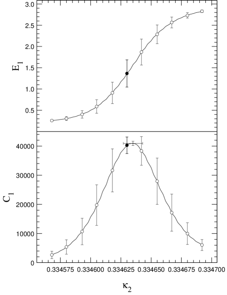
Figure 5 gives an example of the $\kappa_{1}$-energy and of the corresponding specific heat, extrapolated from the simulation point by means of the spectral density method.

Figure 4: Monte Carlo evolution of $E_{1}$ for $\lambda=-0.020$ on the $\phi_{1}$ transition for the $12^{3}$ lattice.

The critical coupling in the thermodynamical limit, i.e. $\kappa_{2}^{c}$, has been obtained from the measurements of $\kappa_{2}(N_{s})$ by means of a fit

$$\kappa_{2}(N_{s})-\kappa_{2}^{c}\sim{N_{s}}^{-1/\nu}~{},$$ (19)

using for the critical exponent $\nu$ its value for first order phase transitions in three dimensions, $\nu=1/3$. The fits turned out to be good in all cases, supporting the first order character of the transition.

Figure 5: $E_{1}$ and $C_{1}$ for $\lambda=-0.020$ on the $\phi_{1}$ transition for the $12^{3}$ lattice by using the spectral density method. The full mark denotes the simulation point, the empty ones are extrapolations thereof.

Having determined the phase diagrams at $T=0$, we passed to the study of the finite temperature case, by simulating asymmetric lattices with $N_{t}<N_{s}$. The values of $N_{t}$ that we considered have been $N_{t}=2,3,4$ for both values of $\lambda$ and $N_{t}=5$ in one case. The values of $N_{s}$ used were the same as for the $T=0$ case, except that for $\lambda=-0.020$ we have sometimes gone up to $N_{s}=24$. The order of the transitions turned out to be always the same as in the corresponding $T=0$ case; in particular, for all $N_{t}$’s we have found the first-order transitions described above for the lower value of $\lambda$. The techniques used to take the thermodynamic limit $N_{s}$ were the same used in the $T=0$ case, except for two differences. Since the scaling parameter was $N_{s}$, while $N_{t}$ was fixed, according to the hypothesis of dimensional reduction and universality, we used the exponents of the Ising model in two dimensions, namely $\nu=1$ and $\omega=4/3$. Similarly, in the case of the first order phase transition encountered for $\lambda=-0.020$, in eq.(19), we used the value of $\nu$ for two dimensions, namely $\nu=1/2$. In both cases we got good fits.

Figure 6: ${\kappa_{2}}^{c}$ as a function of $1/N_{t}$ for $(\lambda_{1}=0.06,~{}\lambda_{2}=0.002,~{}\lambda=-0.016,~{}\kappa_{1}=0.33)$. The points with $1/N_{t}$=0 refer to the symmetric lattices.

Figure 7: ${\kappa_{2}}^{c}$ as a function of $1/N_{t}$ for $(\lambda_{1}=0.06,~{}\lambda_{2}=0.002,~{}\lambda=-0.02,~{}\kappa_{1}=0.33)$. The points with $1/N_{t}$=0 refer to the symmetric lattices.

As far as ISB is concerned, the most important result of the simulations is apparent from figs. 6 and 7: for a constant $\kappa_{1}$, they show that, starting from the symmetric lattices (the points with $1/N_{t}=0$), $\kappa_{2}^{c}$ for the transition of the $\phi_{2}$ field increases monotonically when $N_{t}$ is decreased for both values of $\lambda$ considered; this means that the critical points for $N_{t}$ finite shift deeper and deeper in the ordered region of the $T=0$ model, i.e. raising the temperature disorders the system, as it happens in normal cases (see for a comparison [22]) and contrary to what is required for ISB to occur. Though we have considered a single value of $\kappa_{1}$ in our simulations for finite $N_{t}$’s, we do not expect a different behavior at other points. If for some other value of $\kappa_{1}$ the critical $N_{t}$-line passed below that for the $T=0$ theory, they would have to cross at some point, which would be a very strange fact.

With such a result, there is no need of looking at the continuum limit to rule out ISB. Recalling the comments at the beginning of this section, it is obvious that the CCP’s associated with continuum theories having a symmetric vacuum at $T=0$ cannot cross in any way the $\phi_{2}$ critical lines of the finite $N_{t}$ lattices, for the latter lie in the ordered region of the phase diagram for the symmetric lattices, and not in the disordered one. Then this study indicates that Inverse Symmetry Breaking does not work in this model. However, it is not conclusive about Non Symmetry Restoration because we do not know if the temperature for which the symmetry is restored diverges or not in the continuum limit.

5 Conclusions

Inverse Symmetry Breaking and Symmetry Non-Restoration have recently attracted much interest, mostly due do their potential implications for cosmological scenarios. They are based on the possibility that in multiscalar models some Debye masses can be negative at high temperatures, for suitable choices of the couplings.

In this paper we have presented the results of a Monte Carlo study of ISB in a simple model for two real scalars interacting via a $\lambda\phi^{2}_{1}\phi^{2}_{2}$ coupling, in three euclidean dimensions. The reasons for carrying such a study is that in three dimensions perturbations theory cannot provide any information concerning these phenomena, as it is discussed in Sec.3. In order to have a fully non-perturbative approach to these phenomena, we have thus simulated this scalar model on the lattice and found no trace of ISB. It turned out that for all values of $\lambda$ that we considered the size of the disordered region of the phase diagram increases, when the extension $N_{t}$ of the lattice in the euclidean-time direction is decreased, as it occurs in normal systems, instead of decreasing as required for ISB to occur. Heuristic arguments tell us that this conclusion should be true for the whole parameter space. Another interesting result of our simulations is that, for large negative values of $\lambda$, one of the transitions becomes of first order.

It would be desirable to know if other non-perturbative analytical methods can reproduce our findings. Among the possible approaches we mention here the one based on the Average Effective Action [26], or the CJT formalism [29], that have already been used to study the thermal behavior of two-scalar models in four dimensions [16, 17, 24].

We are currently simulating the model considered in this paper in four dimensions, which is physically the most relevant case. Our efforts are being focused on two issues, both very relevant for Cosmology: one is the study of ISB and SNR and the other is the existence of first order phase transitions at finite temperature. We hope to report soon on this work.

References

- [1] D.A. Kirzhnits and A.D. Linde, Phys. Lett. B42 (1972) 471.
- [2] S. Weinberg, Phys. Rev. D9 (1974) 3357.
- [3] L. Dolan and R. Jackiw, Phys. Rev. D9 (1974) 3320.
- [4] T. W. Kibble, J. Phys. A9 (1976), 1987; Phys. Rep. 67 (1980), 183.
- [5] P. Salomonson, B.-S. Skagerstam and A. Stern, Phys. Lett. B151 (1985) 243.
- [6] G. Dvali, A. Melfo and G. Senjanović, Phys. Rev. Lett. 75 (1996) 4559;
- [7] G. Dvali and G. Senjanović, Phys. Rev. Lett. 74 (1995) 5178;
- [8] P. Langacker and S.-Y. Pi, Phys. Rev. Lett. 45 (1980), 1.
- [9] R.N. Mohapatra and G. Senjanović, Phys. Lett. B89 (1979) 57; Phys. Rev. Lett. 42 (1979) 1651; Phys. Rev. D20 (1979) 3390.
- [10] S.Dodelson and L.Widrow, Mod. Phys. Lett A5 (1990) 1623; Phys. Rev. D42 (1990) 326; Phys. Rev. Lett.64 (1990) 340; S.Dodelson, B.R.Greene and L.M.Widrow, Nucl. Phys. B372 (1992) 347.
- [11] J.Lee and I.Koh, Phys. Rev. D54 (1996), 7153.
- [12] G. Dvali, A. Melfo and G. Senjanović, Phys. Rev. D54 (1996), 7857.
- [13] G. Dvali and K. Tamvakis, Phys. Lett. B378 (1996), 141; B. Bajc and G. Senjanović, Nucl. Phys. Proc. Suppl.52A (1997),246; A. Riotto and G. Senjanović, Phys. Rev. Lett.79 (1997), 349; A. Riotto ”The suprhot, superdense, supersymmetric Universe”, hep-ph/9706296.
- [14] V.A. Kuzmin, M.E. Shaposhnikov and I.I. Tkachev Phys. Rev. 8 (1990) 71.
- [15] G. Bimonte and G. Lozano, Phys. Lett. B366 (1996) 248; Nucl. Phys. B460 (1996), 155.
- [16] G. Amelino-Camelia, Phys. Lett. B388 (1996), 776; Nucl. Phys. B476 (1996), 255.
- [17] T. Ross, Phys. Rev. D54 (1996), 2944; M. Pietroni, N. Rius and N. Tetradis, Phys. Lett. B397 (1997), 119.
- [18] J. Orloff, ” The UV price for symmetry non-restoration”, ENSLAPP-AL-615-96, hep-ph/9611398.
- [19] Y. Fujimoto and S. Sakakibara, Phys. Lett. B151 (1985) 260; E. Manesis and S. Sakakibara, Phys. Lett. B157 (1985) 287; G.A. Hajj and P.N. Stevenson, Phys. Rev. D37 (1988) 413; K.G.Klimenko, Z.Phys. C43 (1989) 581; Theor. Math. Phys. 80 (1989) 929; M.P.Grabowski, Z.Phys. C48 (1990), 505.
- [20] Y. Fujimoto, A. Wipf and H. Yoneyama, Z. Phys. C35 (1987), 351; Phys. Rev. D38 (1988), 2625.
- [21] C. King and L.G. Yaffe, Comm. Math. Phys. 108 (1987), 423; G. Bimonte and G. Lozano, Phys. Lett. B388 (1996), 692.
- [22] G. Bimonte, D. Iñiguez, A. Tarancón and C.L. Ullod, Nucl. Phys. B490 (1997), 701.
- [23] S. Bornholdt, P. Bttner, N. Tetradis and C. Wetterich, “Flow of the Coarse Grained Free Energy for Crossover Phenomena”, CAU-THP-95-38, CERN-TH/96-67, DESY 96-038, HD-THEP-96-05 and cond-mat/9603129.
- [24] S. Bornholdt, N. Tetradis and C. Wetterich, Phys. Rev. D53 (1996), 4552.
- [25] J.I. Kapusta, Finite temperature Field Theory (Cambridge University Press, Cambridge, 1989).
- [26] C. Wetterich, Nucl. Phys. B352 (1991), 529.
- [27] M.B.Einhorn and D.R.T.Jones, Nucl. Phys. B398 (1993), 611.
- [28] K. Binder, Z. Phys. 43 (1981), 119.
- [29] J.M.Cornwall, R.Jackiw and E.Tamboulis, Phys.Rev. D10 (1974), 2428.