NTUA-65/97

OUTP-97-36P

hep-lat/9707027

Dynamical Gauge Symmetry Breaking and Superconductivity in three-dimensional systems

K. Farakos

National Technical University of Athens, Physics Department, Zografou Campus GR-157 73, Athens, Greece,

and
N.E. Mavromatos^∗
University of Oxford, Department of (Theoretical) Physics, 1 Keble Road OX1 3NP, Oxford, U.K.

Abstract
We discuss dynamical breaking of non-abelian gauge groups in three dimensional (lattice) gauge systems via the formation of fermion condensates. A physically relevant example, motivated by condensed-matter physics, is that of a fermionic gauge theory with group $SU(2)\otimes U_{S}(1)\otimes U_{E}(1)$. In the strong $U_{S}(1)$ region, the $SU(2)$ symmetry breaks down to a $U(1)$, due to the formation of a parity-invariant fermion condensate. We conjecture a phase diagram for the theory involving a critical line, which separates the regions of broken $SU(2)$ symmetry from those where the symmetry is restored. In the broken phase, the effective Abelian gauge theory is closely related to an earlier model of two-dimensional parity-invariant superconductivity in doped antiferromagnets. The superconductivity in the model occurs in the Kosterlitz-Thouless mode, since strong phase fluctuations prevent the existence of a local order parameter. Some physical consequences of the $SU(2)\times U_{S}(1)$ phase diagram for the (doping-dependent) parameter space of this condensed-matter model are briefly discussed.

July 1997

^(∗) P.P.A.R.C. Advanced Fellow.

1 Introduction

Gauge symmetry breaking without an elementary Higgs particle, which proceeds via the dynamical formation of fermion condensates, has been a fascinating idea, which however had been tried rather inconclusively, so far, in attempts to understand either chiral symmetry breaking in four-dimensional QCD via a new strong interaction (technicolour) [1], or in the breaking of a local gauge symmetry through the formation of pair condensates in non-singlet channels [2]. In all such scenaria the basic idea is that there exists an energy scale at which the gauge coupling becomes strong enough so as to favour the formation of non-zero fermion condensates $<{\bar{f}}f^{\prime}>$ which are not invariant under the global or local symmetry in question. It is the purpose of this short note to point out that similar scenaria of dynamical gauge symmetry breaking in three-dimensional gauge theories [3] lead to interesting and unconventional superconducting properties of the theory after coupling to electromagnetism [4], and therefore may be of interest to condensed matter community.

In a recent publication [5] we have argued that the doped large-$U$ Hubbard (antiferromagnetic) models possess a hidden local non-Abelian $SU(2)\times U_{S}(1)$ phase symmetry related to spin interactions. This symmetry was discovered through a generalised slave-fermion ansatz for spin-charge separation [6], which allows intersublattice hopping for holons, and hence spin flip . The spin-charge separation may be physically interpreted as implying an effective ‘substructure’ of the electrons due to the many body interactions in the medium. This sort of idea, originating from Anderson’s RVB theory of spinons and holons [6], was also pursued recently by Laughlin, although from a (formally at least) different perspective [8].

The effective long wavelength model of such a statistical system is remarkably similar to a three-dimensional gauge model of particle physics proposed in ref. [3] as a toy example for chiral symmetry breaking in QCD. In that work, it has been argued that dynamical generation of a fermion mass gap due to the $U_{S}(1)$ subgroup of $SU(2)\times U_{S}(1)$ breaks the $SU(2)$ subgroup down to a $\sigma_{3}-U(1)$ group, where $\sigma_{3}$ is the $2\times 2$ Pauli matrix. From the particle-theory view point this is a Higgs mechanism without an elementary Higgs excitation. The analysis carries over to the condensed-matter case, if one associates the mass gap to the holon condensate [5]. The resulting effective theory of the light degrees of freedom is then similar to the continuum limit of [4] describing unconventional parity-conserving superconductivity.

Apart from their condensed-matter applications, however, we believe that such patterns of symmetry breaking are also of interest to the particle-physics community. For instance, it is known that high-temperature gauge theories in four dimensions become effectively three-dimensional euclidean systems. Therefore, one cannot exclude the possibility that the scenaria discussed here, and in refs. [3, 4], might be of relevance to this case in the future. For this reason we consider it as useful to expose the particle-physics community to the above ideas through this short note.

The structure of the article is as follows: in sec. 2 we review briefly the dynamical symmetry breaking patterns of $SU(2)\times U_{S}(1)$ model on the lattice. In sec. 3 we discuss the phase diagram of the theory and argue in favour of the existence of a critical line separating the broken-$SU(2)$ phase from that where the symmetry is restored. In sec. 4 we present the superconducting properties of the broken phase upon coupling the system to electromagnetic potentials. Finally in section 5, instead of conclusions, we discuss very briefly the application of these ideas to a specific model in condensed matter physics, which might have some relevance to the physics of high-temperature superconductors. The interested reader may find details on the physics of this model in ref. [5].

2 Dynamical Non-Abelian Gauge Symmetry Breaking on the Lattice

To understand the nature of the non-Abelian gauge symmetries under consideration it is instructive to start with the simpler case of a local Abelian gauge theory, invariant under a group $U_{S}(1)$, which has a global $U(2)$ symmetry. Eventually we shall gauge this non-Abelian symmetry and make contact with the lattice models [5]. We, therefore, begin by considering the following three-dimensional continuum lagrangian [3, 5]:

$${\cal L}=-\frac{1}{4}(F_{\mu\nu})^{2}+{\overline{\Psi}}D_{\mu}\gamma_{\mu}\Psi-m_{0}{\overline{\Psi}}\Psi$$ (1)

where $D_{\mu}=\partial_{\mu}-ig_{1}a_{\mu}^{S}$, and $F_{\mu\nu}$, is the corresponding field strength for the abelian (termed ‘statistical’) gauge field $a^{S}_{\mu}$. In the statistical model of ref. [5], the field $a_{S}$ is responsible for fractional statistics of the pertinent (holon) excitationson of the planar doped antiferromagnet. Anticipating the connection of (1) with the (naive) continuum limit of an appropriate stastistical (lattice) system, we may take the fermions $\Psi$ to be four-component spinors, due to lattice doubling. It is in this formalism that the global $U(2)$ symmetry will be constructed [3, 5]. The parity-conserving bare-mass $m_{0}$ term has been added by hand to facilitate Monte-Carlo studies [9] of dynamically-generated fermion masses as a result of the formation of fermion condensates $<{\overline{\Psi}}\Psi>$ by the strong $U_{S}(1)$ coupling. The $m_{0}=0$ limit should be taken at the end. The $\gamma_{\mu}$, $\mu=0,1,2$, matrices span the reducible $4\times 4$ representation of the Dirac algebra in three dimensions in a fermionic theory with an even number of fermion flavours [10]: $\gamma^{0}=\left(\begin{array}[]{cc}{\bf\sigma}_{3}\qquad{\bf 0}\\ {\bf 0}\qquad-{\bf\sigma}_{3}\end{array}\right)\qquad\gamma^{1}=\left(\begin{array}[]{cc}i{\bf\sigma}_{1}\qquad{\bf 0}\\ {\bf 0}\qquad-i{\bf\sigma}_{1}\end{array}\right),\gamma^{2}=\left(\begin{array}[]{cc}i{\bf\sigma}_{2}\qquad{\bf 0}\\ {\bf 0}\qquad-i{\bf\sigma}_{2}\end{array}\right)$ where ${\bf\sigma}$ are $2\times 2$ Pauli matrices and the (continuum) space-time is taken to have Minkowskian signature. As well known [10] there exist two $4\times 4$ matrices which anticommute with $\gamma_{\mu}$,$\mu=0,1,2$, and generate a ‘chiral’ symmetry in a theory with even number of fermion species: $\gamma_{3}~{}=\left(\begin{array}[]{cc}0\qquad{\bf 1}\\ {\bf 1}\qquad 0\end{array}\right),\qquad\gamma_{5}=i\left(\begin{array}[]{cc}0\qquad{\bf 1}\\ {\bf-1}\qquad 0\end{array}\right)$, where the substructures are $2\times 2$ matrices.

The set of generators

$${\cal G}=\{{\bf 1},\gamma_{3},\gamma_{5},\Delta\equiv i\gamma_{3}\gamma_{5}\}$$ (2)

form [3] a global $U(2)\simeq SU(2)\times U_{E}(1)$ symmetry. The identity matrix ${\bf 1}$ generates the $U_{E}(1)$ subgroup, while the other three form the SU(2) part of the group. In the statistical model for (magnetic) superconductivity of ref. [5], which we shall describe briefly below, the global $U_{E}(1)$ corresponds to the electromagnetic charge of the holons, and can be gauged by coupling the system to an external electromagnetic potential $A_{\mu}$.

In two-component notation for the spinors $\Psi_{i}$, the bilinears

$${\cal A}_{1}\equiv-i[{\overline{\Psi}}_{1}\Psi_{2}-{\overline{\Psi}}_{2}\Psi_{1}],\qquad{\cal A}_{2}\equiv{\overline{\Psi}}_{1}\Psi_{2}+{\overline{\Psi}}_{2}\Psi_{1},\qquad{\cal A}_{3}\equiv{\overline{\Psi}}_{1}\Psi_{1}-{\overline{\Psi}}_{2}\Psi_{2},$$ (3)

$${\cal F}_{1\mu}\equiv{\overline{\Psi}}_{1}\sigma_{\mu}\Psi_{2}+{\overline{\Psi}}_{2}\sigma_{\mu}\Psi_{1},\qquad{\cal F}_{2\mu}\equiv i[{\overline{\Psi}}_{1}\sigma_{\mu}\Psi_{2}-{\overline{\Psi}}_{2}\sigma_{\mu}\Psi_{1}],$$

$${\cal F}_{3\mu}\equiv{\overline{\Psi}}_{1}\sigma_{\mu}\Psi_{1}-{\overline{\Psi}}_{2}\sigma_{\mu}\Psi_{2},$$

transform as triplets under $SU(2)$.

On the other hand, the $SU(2)$ singlets are given by the bilinears:

$${\cal A}_{4}\equiv{\overline{\Psi}}_{1}\Psi_{1}+{\overline{\Psi}}_{2}\Psi_{2},\qquad{\cal F}_{4,\mu}\equiv{\overline{\Psi}}_{1}\sigma_{\mu}\Psi_{1}+{\overline{\Psi}}_{2}\sigma_{\mu}\Psi_{2}~{},\qquad\mu=0,1,2$$ (4)

i.e. the singlets are the parity violating mass term, and the four-component fermion number.

One may gauge the above group $SU(2)\times U_{S}(1)\times U_{E}(1)$, where, we remind the reader once again that the electromagnetic symmetry $U_{E}(1)$ is gauged by coupling the system to external electromagnetic potentials:

$${\cal L}_{2}\equiv=-\frac{1}{4}(F_{\mu\nu})^{2}-\frac{1}{4}({\cal G}_{\mu\nu})^{2}+{\overline{\Psi}}D_{\mu}\gamma_{\mu}\Psi-m_{0}{\overline{\Psi}}\sigma_{3}\Psi$$ (5)

where now $D_{\mu}=\partial_{\mu}-ig_{1}a_{\mu}^{S}-ig_{2}\sigma^{a}B_{a,\mu}-\frac{e}{c}A_{\mu}$, $B_{\mu}^{a}$ is the gauge potential of the local (‘spin’) $SU(2)$ group, and ${\cal G}_{\mu\nu}$ is the corresponding field strength. The fermions $\Psi$ are now, and in what follows, viewed as two-component spinors. Once we gauged the $SU(2)$ group, the colour structure is up and above the space-time Dirac structure, and in two-component notation the $SU(2)$ group is generated by the familiar $2\times 2$ Pauli matrices $\sigma^{a}$, $a=1,2,3$. In this way, the fermion condensate ${\cal A}_{3}$ can be generated dynamically by means of a strongly-coupled $U_{S}(1)$. In this context, energetics prohibits the generation of a parity-violating gauge invariant $SU(2)$ term [16], and so a parity-conserving mass term necessarily breaks [3] the $SU(2)$ group down to a $\sigma_{3}-U(1)$ sector [4], generated by the $\sigma_{3}$ Pauli matrix in two-component notation.

The above symmetry breaking patterns may be proven analytically [3] on the lattice, in the strong $U_{S}(1)$ limit, $\beta_{1}\rightarrow 0$. The lattice lagrangian, corresponding to the continuum lagrangian (5), assumes the form:

$$S=\frac{1}{2}K\sum_{i,\mu}[{\overline{\Psi}}_{i}(-\gamma_{\mu})U_{i,\mu}V_{i,\mu}\Psi_{i+\mu}+$$ (6)

$${\overline{\Psi}}_{i+\mu}(\gamma_{\mu})U^{\dagger}_{i,\mu}V^{\dagger}_{i,\mu}\Psi_{i}]$$

$$+\beta_{1}\sum_{p}(1-trU_{p})+\beta_{2}\sum_{p}(1-trV_{p})$$

where $\mu=0,1,2$, $U_{i,\mu}=exp(i\theta_{i,\mu})$ represents the statistical $U_{S}(1)$ gauge field, $V_{i,\mu}=exp(i\sigma^{a}B_{a})$ is the $SU(2)$ gauge field, The fermions $\Psi$ are taken to be two-component (Wilson) spinors, in both Dirac and colour spaces [3, 5]. Here we have passed onto a three-dimensional Euclidean lattice formalism, in which ${\overline{\Psi}}$ is identified with $\Psi^{\dagger}$. In this convention the bilinears (3),(4) are hermitean quantities.

In the strong-coupling limit, $\beta_{1}=0$ the field $U_{S}(1)$ field may be integrated out analytically in the path integral with the result  [3]:

$$Z=\int dVd{\overline{\Psi}}d\Psi exp(-S_{eff})$$ (7)

where

$$S_{eff}=\beta_{2}\sum_{p}(1-trV_{p})-\sum_{i,\mu}{\rm ln}I^{tr}_{0}(2\sqrt{y_{i\mu}})$$ (8)

$$y_{i\mu}=-\frac{K^{2}}{4}tr[M^{(i)}(-\gamma_{\mu})V_{i\mu}M^{(i+\mu)}(\gamma_{\mu})V_{i\mu}^{\dagger}]$$

where and

$$M^{(i)}_{ab,\alpha\beta}\equiv\Psi_{i,b,\beta}{\overline{\Psi}}_{i,a,\alpha},~{}~{}a,b={\rm colour},~{}\alpha,\beta={\rm Dirac},~{}i={\rm lattice~{}site}$$ (9)

are the meson states, and ${\rm ln}I^{tr}_{0}$ denotes the logarithm of the zeroth order Modified Bessel function [11], truncated to an order determined by the number of the Grassmann (fermionic) degrees of freedom in the problem [12]. In our case, due to the $SU(2)$ and spin quantum numbers of the lattice spinors $\Psi$, one should retain terms in $-{\rm ln}I^{tr}_{0}$ up to ${\cal O}(y^{4})$:

$$-{\rm ln}I^{tr}_{0}(2\sqrt{y_{i\mu}})=-y_{i\mu}+\frac{1}{4}y^{2}_{i\mu}-\frac{1}{9}y_{i\mu}^{3}+\frac{11}{192}y_{i\mu}^{4}$$ (10)

The above expression is an exact result, irrespectively of the magnitude of $y_{i\mu}$.

The low-energy (long-wavelength) effective action is written as a path-integral in terms of gauge and meson fields, $Z=\int[dVdM]exp(-S_{eff}+\sum_{i}tr{\rm ln}M^{(i)})$, where the meson-dependent term comes from the Jacobian in passing from fermion integrals to meson ones [12].

To identify the symmetry-breaking patterns of the gauge theory (10) one may concentrate on the lowest-order terms in $y_{i\mu}$, which will yield the gauge boson masses. Higher-order terms will describe interactions, as we shall discuss in the next section. Keeping thus only the linear term in the expansion yields [3]:

$${\rm ln}I^{trunc}_{0}(2\sqrt{y_{i\mu}})|_{linear}=y_{i\mu}=-\frac{1}{4}K^{2}tr[M^{(i)}(-\gamma_{\mu})V_{i\mu}M^{(i+\mu)}(\gamma_{\mu})V_{i\mu}^{\dagger}]$$ (11)

It is evident that symmetry-breaking patterns for $SU(2)$ will emerge out of a non zero VEV for the meson matrices $M^{(i)}$.

Lattice simulations of the model (6), with only a global $SU(2)$ symmetry, in the strong $U_{S}(1)$ coupling limit $\beta_{1}=0$, and in the quenched approximation for fermions, have shown [9] that the states generated by the bilinears ${\cal A}_{1}$ and ${\cal A}_{2}$ (3) are massless, and therefore correspond to Goldstone Bosons, while the state generated by the bilinear ${\cal A}_{3}$ is massive. The fact that members of the triplet SU(2) representation acquire different masses is already evidence for symmetry breaking. To demonstrate this explicitly one uses the following expansion for the meson states in terms of the $SU(2)$ bilinears (3),(4) [3]:

$$M^{(i)}={\cal A}_{3}(i)\sigma_{3}+{\cal A}_{1}(i)\sigma_{1}+{\cal A}_{2}(i)\sigma_{2}+{\cal A}_{4}(i){\bf 1}+$$ (12)

$${\cal F}_{4,\mu}(i)\gamma^{\mu}+{\cal F}_{1,\mu}(i)\gamma^{\mu}\sigma_{1}+{\cal F}_{2,\mu}(i)\gamma^{\mu}\sigma_{2}+{\cal F}_{3,\mu}(i)\gamma^{\mu}\sigma_{3}$$

with $\mu=0,1,2$, $\gamma_{\mu}$ are hermitean Dirac (space-time) $2\times 2$ matrices, and $\sigma_{a}$, $a=1,2,3$ are the (hermitean) $2\times 2$ SU(2)-‘colour’ Pauli matrices. Note that the VEV of the matrix $<M^{(i)}>=u\sigma_{3}$ is proportional to the chiral condensate. Upon substituting (12) in (11), taking into account that the SU(2) link variables may be expressed as $V_{i\mu}=cos(|{\bf B}_{i\mu}|)+i{\bf\sigma}.{\bf B}_{i\mu}sin(|{\bf B}_{i\mu}|)/|{\bf B}_{i\mu}|$, and performing a naive perturbative expansion over the fields ${\bf B}$ one finds:

$${\rm ln}I^{trunc}_{0}(2\sqrt{y_{i\mu}})|_{linear}\propto K^{2}u^{2}[(B^{1}_{i\mu})^{2}+(B^{2}_{i\mu})^{2}]~{}+~{}{\rm interaction~{}terms}$$ (13)

From this it follows that two of the $SU(2)$ gauge bosons, namely the $B^{1}$,$B^{2}$ become massive, with masses proportional to the chiral condensate $u$:

$${\rm B^{1,2}~{}boson~{}masses}\propto K^{2}u^{2}$$ (14)

whilst the gauge boson $B^{3}$ remains massless. Thus, $SU(2)$ is broken down to a $U(1)$ subgroup, generated by the $\sigma_{3}$ Pauli matrix.

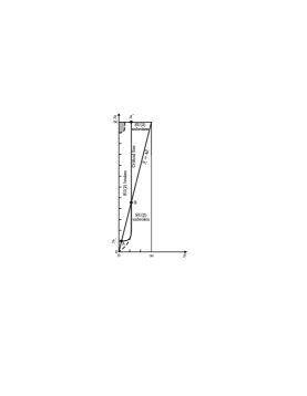
Figure 1: Phase diagram for the $SU(2)\times U_{S}(1)$ gauge theory. The critical line separates the phase of (dynamically) broken $SU(2)$ symmetry from the unbroken phase. Its shape is conjectural at this stage, in particular with respect to the order of magnitude of $\beta_{2}^{c}$. The shaded region has been analysed in ref. [3]. The dashed line represents a probable critical line in the case of the statistical model of ref. [5]. The straight line indicates the specific relation of the coupling constants in that model.

3 Phase Diagram of $SU(2)\times U_{S}(1)$ Theory

The reader might have noticed a similarity between the gauge fermion interaction terms (11) and the corresponding Higgs-fermion interactions in the adjoint Higgs model [13]. The adjoint Higgs model is characterized by a critical value of $K$ above which spontaneous symmetry breaking occurs. In our case, however, as we shall argue below, the system is always in the broken phase in the region $\beta_{2}=\infty,\beta_{1}=0$, independently of $K$.

To prove this, we consider the situation along the vertical axis of the phase diagram of fig. 1 at $\beta_{1}=0$. The effective potential depends on the variable $y$ defined in (8). To determine its form, in terms of the condensate, one uses the expansion (12) and concentrates on the terms of the $SU(2)$ triplet, ${\cal A}_{i}\equiv\Phi_{i},i=1,2,3$. This triplet plays a rôle analogous to that of the Higgs triplet in the adjoint Higgs model [13]. In that model, one of the members of the triplet, along the $\sigma_{3}$ direction of $SU(2)$, acquires a vacuum expectation value, exactly as it happens in our case above. The form of the effective potential in the naive continuum limit (lattice spacing $a\rightarrow 0$ ) and in the weak $SU(2)$ case may be found from (10) by expanding the $SU(2)$ link variables $U_{ij}\simeq 1+O(agA)$, where $g$ is the group coupling, $a$ is the lattice spacing and $A$ is the gauge potential. Taking the limit $g\rightarrow 0$ ($\beta_{2}=\infty$) one then obtains $y(x)\sim\frac{K^{2}}{2}Tr\Phi^{2}(x)=K^{2}\sum_{i=1}^{3}\Phi_{i}^{2}$. The tree-level effective potential is then:

$$V_{eff}=-3K^{2}R^{2}+\frac{3}{4}K^{4}R^{4}-\frac{1}{3}K^{6}R^{6}+\frac{33}{192}K^{8}R^{8}$$ (15)

$$R^{2}\equiv\frac{1}{2}Tr\Phi^{2}=\sum_{i=1}^{3}\Phi_{i}^{2}$$

The coefficient $3$ originates from the summation over the three link variables at each site of our three-dimensional lattice gauge theory. The potential (15) has the characteristic double-well shape of a symmetry-breaking (adjoint) Higgs potential, with a non-trivial minimum at $KR\simeq 1.3$ (c.f. figure 2). Hence, for any value of $K$ there is always a corresponding Parity-invariant condensate, which is inversely proportional to $K$, implying that there is no critical value of $K$ above which the symmetry changes. The system always remains in a single (broken $SU(2)$ symmetry) phase in the region $\beta_{1}=0,\beta_{2}={\rm large}$, irrespectively of the strength of $K$. The reason for this behaviour, in contrast to the adjoint Higgs case [13], where a critical $K$ does exist, is the specific form of the effective potential in the gauge case: the condensate interaction terms originate from a single gauge-fermion term (11), and their coupling constant is determined by $K$. In contrast, the adjoint Higgs model is characterised by an independent coupling for the Higgs interactions [13], and for certain regions of the parameters a change in symmetry occurs.

Figure 2: The effective potential (15) in the case $\beta_{1}=0$, $\beta_{2}=\infty$. The system is in the broken-$SU(2)$-symmetry phase for any $K$.

The incorporation of the gauge interactions will change the situation, and induce non-trivial dynamics which may result in a change in symmetry for some regions of the gauge coupling constants. From the previous result (15), and the discussion in section 2, it becomes clear that for weak $SU(2)$ and strong enough $U_{S}(1)$ the $SU(2)$ symmetry is broken down to a $U(1)$ subgroup [3]. The non-trivial issue here is whether there exist critical (inverse) couplings $\beta_{i}^{c},i=1,2$, above which the symmetry is restored. Let us first concentrate on the axis $\beta_{2}=\infty$, $\beta_{1}={\rm free}$. According to earlier analyses, either in the continuum or on the lattice [10, 14, 15], there appears to be a critical coupling $\beta_{1}^{c}$ on this axis above which dynamical mass generation due to the $U_{S}(1)$ group cannot take place. This is depicted in figure 1.

The situation concering the $\beta_{2}$ coupling is more complicated. Let us first concentrate on the region of strong $SU(2)$, $\beta_{2}=0$, keeping $U_{S}(1)$ arbitrary (bottom horizontal axis of fig. 1). In this part of the phase diagram one can integrate out the (strongly coupled) $SU(2)$ gauge fields to derive an effective action for the fermion and $U_{S}(1)$ gauge fields. The $SU(2)$ path integration is performed along the lines of ref. [12]. In the strong coupling limit for $SU(2)$, $\beta_{2}=0$, the effective action, obtained after integration of the $SU(2)$ gauge fields, reduces to the a sum of one-link contributions, $S_{eff}=S_{eff}(A,{\overline{A}})$, with

$$A_{\mu}(x)^{a}_{b}={\overline{\Psi}}_{b}(x+a)\gamma_{\mu}U^{\dagger}_{x,\mu}\Psi^{a}(x)\qquad{\overline{A}}_{\mu}(x)^{a}_{b}={\overline{\Psi}}_{b}(x)(-\gamma_{\mu})U_{x,\mu}\Psi^{a}(x+a)$$ (16)

where $U_{x,\mu}$ denotes the $U_{S}(1)$ group element, $a$ is the lattice spacing, and the latin indices $a,b$ are colour $SU(2)$ indices. For the $SU(N)$ case the quantity $exp(-S_{eff})$ is known in an expansion over $A$, ${\overline{A}}$ [12]. This will be sufficient for our purposes here:

$$S_{eff}=\frac{1}{N}Tr({\overline{A}}A)+\frac{1}{2N(N^{2}-1)}[-Tr[({\overline{A}}A)^{2}]+\frac{1}{N}(Tr[{\overline{A}}A])^{2}]+\dots+\frac{1}{N!}(detA+det{\overline{A}})+\dots$$ (17)

The determinant terms are associated with baryonic states [12]. We also note that for the $U(N)$ case the determinant terms are absent. In the phase diagram of fig. 1 the $U(2)$ case occurs at the point $\beta_{2}\rightarrow 0,\beta_{1}\rightarrow 0$. In our discussion below we shall approach that point asymptotically, by working on the $\beta_{2}=0$ line, and assuming $\beta_{1}\neq 0$. We first notice that the Abelian phase factors of the $U_{S}(1)$ interactions cancel from the expressions for the traces of $A$, ${\overline{A}}$ in the effective action (17). Moreover, from the discussion of section 2, we know that the $SU(2)$ (strong-coupling) integration cannot produce a parity-invariant condensate, since the latter is not an $SU(2)$ singlet [3]. The resulting effective action should be expressible in terms of $SU(2)$ invariant fields. Thus, on the axis $\beta_{2}=0$ there is no possibility for the $U_{S}(1)$ group to generate a fermion condensate. This implies that for very strong $SU(2)$ group the symmetry is restored for arbitrary $U_{S}(1)$ couplings. This observation, together with the fact that for weak $SU(2)$ couplings there is dynamical formation of parity invariant fermion condensates along the axis $\beta_{1}=0$ [10, 4, 3, 5], implies the existence of a critical $\beta_{2}^{c}$ above which the $SU(2)$ symmetry is restored. The issue is whether this critical coupling is finite or it occurs at infinity. This issue requires proper lattice simulations, which fall beyond the scope of the present work. However in certain specific models, like the one in ref. [5], this issue might be resolved, as we shall discuss in section 5.

The conclusion of the above analysis, therefore, is that there exists a critical line in the phase diagram of fig. 1, which separates the $SU(2)$-broken phase of the theory from the phase where the symmetry is restored. Its precise shape is conjectural at this stage and can only be determined by finite $\beta_{2}$ calculations. This is in progress.

Having discussed the situation concerning the parity-invariant condensate, one should now examine the possibility of the parity-violating one ($SU(2)$ singlet, ${\cal A}_{4}\equiv\phi$) which might be generated by the non-Abelian group. However, for the case of a single fermion flavour, $N_{f}=1$, which is the case we have been concentating so far, this is not possible. Energetics prohibits the dynamical generation of the $SU(2)$-singlet parity-violating condensate [16, 10], except in the case where there exist non-zero parity-violating source terms in the lattice action [17]. This is consistent with the form of the effective action (17). Indeed, the trace terms in (17) depend only on the combination $A{\overline{A}}$ which is parity invariant. Moreover, as can be easily seen, the determinant terms do not contain $\phi$:

$$detA+det{\overline{A}}=-\frac{K^{2}}{4}[{\overline{\Psi}}_{1,\alpha}(x){\overline{\Psi}}_{2,\delta}(x)(\gamma_{\mu})^{\alpha}_{\beta}(\gamma^{\mu})^{\delta}_{\eta}\Psi_{1}^{\beta}(x+{\hat{\mu}})\Psi_{2}^{\eta}(x+{\hat{\mu}})e^{2i\theta_{x,\mu}}-$$ (18)

$${\overline{\Psi}}_{2,\delta}(x){\overline{\Psi}}_{1,\alpha}(x)(\gamma_{\mu})^{\delta}_{\beta}(\gamma^{\mu})^{\alpha}_{\eta}\Psi_{1}^{\beta}(x+{\hat{\mu}})\Psi_{2}^{\eta}(x+{\hat{\mu}})e^{2i\theta_{x,\mu}}+$$

$${\overline{\Psi}}_{1,\alpha}(x+{\hat{\mu}}){\overline{\Psi}}_{2,\delta}(x+{\hat{\mu}})(\gamma_{\mu})^{\alpha}_{\beta}(\gamma^{\mu})^{\delta}_{\eta}\Psi_{1}^{\beta}(x)\Psi_{2}^{\eta}(x)e^{-2i\theta_{x,\mu}}-$$

$${\overline{\Psi}}_{2,\delta}(x+{\hat{\mu}}){\overline{\Psi}}_{1,\alpha}(x+{\hat{\mu}})(\gamma_{\mu})^{\delta}_{\beta}(\gamma^{\mu})^{\alpha}_{\eta}\Psi_{1}^{\beta}(x)\Psi_{2}^{\eta}(x)e^{-2i\theta_{x,\mu}}]$$

where ${\hat{\mu}}$ denotes the unit step in the $\mu$ direction, Greek indices are spinor indices, $1,2$ denote colour $(SU(2))$ indices, and $\theta_{i,\mu}$ is the $U_{S}(1)$ gauge phase. This expression depends on the baryonic states [12] ${\cal B}_{\alpha\beta}\propto\epsilon_{ab}\Psi_{\alpha}^{a}\Psi_{\beta}^{b}$, $\alpha,\beta$ spinor indices, $a,b$ colour indices, and, hence, does not contain the parity-violating ${\cal A}_{4}$ meson state (4) ${\cal A}_{4}\sim{\overline{\Psi}}_{1}\Psi_{1}+{\overline{\Psi}}_{2}\Psi_{2}$. Thus, the form of the effective action (17) in our case is consistent with the impossibility of the spontaneous breaking of parity in vector-like theories in odd dimensions [16].

A final point concerns the multiflavour fermionic case, $N_{f}>1$. In the case of an even flavour number it is possible for a strong $SU(2)$ group to generate a parity invariant combination of fermion masses, if $N_{f}/2$ flavours get positive masses and $N_{f}/2$ get masses equal in magnitude but opposite in sign [10, 16]. This completes our (preliminary) study of the phase diagram (fig. 1) of the $SU(2)\times U_{S}(1)$ model of a gauged chiral symmetry considered above.

4 Superconducting Properties

As a final topic of our generic analysis of three-dimensional gauge models we would like to discuss the superconducting consequences of the above dynamical breaking patterns of the $SU(2)$ group. Superconductivity is obtained upon coupling the system to external elelctromagnetic potentials, which leads to the presence of an additional gauge-symmetry, $U_{E}(1)$, that of ordinary electromagnetism.

Figure 3: Anomalous one-loop Feynman matrix element, leading to a Kosterlitz-Thouless-like breaking of the electromagnetic $U_{E}(1)$ symmetry, and thus superconductivity, once a fermion mass gap opens up. The wavy line represents the $SU(2)$ gauge boson $B_{\mu}^{3}$, which remains massless, while the blob denotes an insertion of the fermion-number current $J_{\mu}={\overline{\Psi}}\gamma_{\mu}\Psi$. Continuous lines represent fermions.

Upon the opening of a mass gap in the fermion (hole) spectrum, one obtains a non-trivial result for the following Feynman matrix element: ${\cal S}^{a}=<B^{a}_{\mu}|J_{\nu}|0>,~{}a=1,2,3$, with $J_{\mu}={\overline{\Psi}}\gamma_{\mu}\Psi$, the fermion-number current. Due to the colour-group structure, only the massless $B^{3}_{\mu}$ gauge boson of the $SU(2)$ group, corresponding to the $\sigma_{3}$ generator in two-component notation, contributes to the matrix element. The non-trivial result for the matrix element ${\cal S}^{3}$ arises from an anomalous one-loop graph, depicted in figure 3, and it is given by [18, 4]:

$${\cal S}^{3}=<B^{3}_{\mu}|J_{\nu}|0>=({\rm sgn}{M})\epsilon_{\mu\nu\rho}\frac{p_{\rho}}{\sqrt{p_{0}}}$$ (19)

where $M$ is the parity-conserving fermion mass (holon condensate), generated dynamically by the $U_{S}(1)$ group. As with the other Adler-Bell-Jackiw anomalous graphs in gauge theories, the one-loop result (19) is exact and receives no contributions from higher loops [18].

This unconventional symmetry breaking (19), does not have a local order parameter [18, 4], since the latter is inflicted by strong phase fluctuations, thereby resembling the Kosterlitz-Thouless mode of symmetry breaking [19]. The massless Gauge Boson $B_{\mu}^{3}$ of the unbroken $\sigma_{3}-U(1)$ subgroup of $SU(2)$ is responsible for the appearance of a massless pole in the electric current-current correlator [4], which is the characteristic feature of any superconducting theory. As discussed in ref. [4], all the standard properties of a superconductor, such as the Meissner effect, infinite conductivity, flux quantization, London action etc. are recovered in such a case. The field $B^{3}_{\mu}$, or rather its dual $\phi$ defined by $\partial_{\mu}\phi\equiv\epsilon_{\mu\nu\rho}\partial_{\nu}B^{3}_{\rho}$, can be identified with the Goldstone Boson of the broken $U_{em}(1)$ (electromagnetic) symmetry [4].

5 Application to Doped Planar Antiferromagnets

Before closing we would like to discuss how these results can be connected with the low-energy limit of doped antiferromagnetic planar systems of relevance to the physics of high-temperature superconductors. We shall be very brief in our discussion here. For more details we refer the reader to ref. [5] and references therein. The model considered in [5] was the strong-U Hubbard model, describing doped antiferromegnets with the constraint of no more than one elelctron per lattice site. The key suggestion in ref. [5], which lead to the non-abelian gauge symmetry structure for the doped antiferromagnet, was the slave-fermion spin-charge separation ansatz for physical electron operators at each lattice site $i$ [5]:

$$\chi_{\alpha\beta,i}\equiv\left(\begin{array}[]{cc}c_{1}\qquad c_{2}\\ c_{2}^{\dagger}\qquad-c_{1}^{\dagger}\end{array}\right)_{i}\equiv{\widehat{\psi}}_{\alpha\gamma,i}{\widehat{z}}_{\gamma\beta,i}=\left(\begin{array}[]{cc}\psi_{1}\qquad\psi_{2}\\ -\psi_{2}^{\dagger}\qquad\psi_{1}^{\dagger}\end{array}\right)_{i}~{}\left(\begin{array}[]{cc}z_{1}\qquad-{\overline{z}}_{2}\\ z_{2}\qquad{\overline{z}}_{1}\end{array}\right)_{i}$$ (20)

where $c_{\alpha}$, $\alpha=1,2$ are electron anihilation operators, the Grassmann variables $\psi_{i}$, $i=1,2$ play the rôle of holon excitations, while the bosonic fields $z_{i},i=1,2,$ represent magnon excitations [6]. The ansatz (20) has spin-electric-charge separation, since only the fields $\psi_{i}$ carry electric charge. This ansatz characterizes the proposal of ref. [5] for the dynamics underlying doped antiferromagnets. In this context, the holon fields ${\widehat{\psi}}_{\alpha\beta}$ may be viewed as substructures of the physical electron $\chi_{\alpha\beta}$ [8], in close analogy to the ‘quarks’ of $QCD$.

As argued in ref. [5] the ansatz is characterised by the following local phase (gauge) symmetry structure:

$$G=SU(2)\times U_{S}(1)\times U_{E}(1)$$ (21)

The local SU(2) symmetry is discovered if one defines the transformation properties of the ${\widehat{z}}_{\alpha\beta}$ and ${\widehat{\psi}}^{\dagger}_{\alpha\beta}$ fields to be given by left multiplication with the $SU(2)$ matrices, and pertains to the spin degrees of freedom. The local $U_{S}(1)$ ‘statistical’ phase symmetry, which allows fractional statistics of the spin and charge excitations. This is an exclusive feature of the three dimensional geometry, and is similar in spirit to the bosonization technique of the spin-charge separation ansatz of ref. [20], and allows the alternative possibility of representing the holes as slave bosons and the spin excitations as fermions. Finally the $U_{E}(1)$ symmetry is due to the electric charge of the holons.

The pertinent long-wavelength gauge model, describing the low-energy dynamics of the large-U Hubbard antiferromagnet, in the spin-charge separation phase (20), assumes the form [5]:

$$H_{HF}=\sum_{<ij>}tr\left[(8/J)\Delta^{\dagger}_{ij}\Delta_{ji}+K(-t_{ij}(1+\sigma_{3})+\Delta_{ij}){\widehat{\psi}}_{j}V_{ji}U_{ji}{\widehat{\psi}}_{i}^{\dagger}\right]+$$ (22)

$$\sum_{<ij>}tr\left[K{\overline{\widehat{z}}}_{i}V_{ij}U_{ij}{\widehat{z}}_{j}\right]+h.c.$$

where $J$ is the Heisneberg antiferromagnetic interaction, $K$ is a normalization constant, and $\Delta_{ij}$ is a Hubbard-Stratonovich field that linearizes four-electron interaction terms in the original Hubbard model, and $U_{ij}$,$V_{ij}$ are the link variables for the $U_{S}(1)$ and $SU(2)$ groups respectively. The conventional lattice gauge theory form of the action (22) is derived upon freezing the fluctuations of the $\Delta_{ij}$ field [5], and integrating out the magnon fields, $z$, in the path integral. This latter operation yields appropriate Maxwell kinetic terms for the link variables $V_{ij}$, $U_{ij}$, in a low-energy derivative expansion  [21, 22]. On the lattice such kinetic terms are given by plaquette terms of the form [5]:

$$\sum_{p}\left[\beta_{SU(2)}(1-TrV_{p})+\beta_{U_{S}(1)}(1-TrU_{p})\right]$$ (23)

where $p$ denotes sum over plaquettes of the lattice, and $\beta_{U_{S}(1)}\equiv\beta_{1}$, $\beta_{SU(2)}\equiv\beta_{2}=4\beta_{1}$ are the dimensionless (in units of the lattice spacing) inverse square couplings of the $U_{S}(1)$ and $SU(2)$ groups, respectively [5]. The above relation between the $\beta_{i}$’s is due to the specific form of the $z$-dependent terms in (22), which results in the same induced couplings $g_{SU(2)}^{2}=g_{U_{S}(1)}^{2}$. Moreover, there is a non-trivial connection of the gauge group couplings to $K$ [5]:

$$K\propto g_{SU(2)}^{2}=g_{U_{S}(1)}^{2}\propto J\eta$$ (24)

with $\eta$ the doping concentration in the sample [5, 25]. To cast the symmetry structure in a form that is familiar to particle physicists, one may change representation of the $SU(2)$ group, and instead of working with $2\times 2$ matrices in (20), one may use a representation in which the fermionic matrices ${\widehat{\psi}}_{\alpha\beta}$ are represented as two-component (Dirac) spinors in ‘colour’ space:

$${\tilde{\Psi}}_{1,i}^{\dagger}=\left(\psi_{1}~{}~{}-\psi_{2}^{\dagger}\right)_{i},~{}~{}~{}~{}{\tilde{\Psi}}_{2,i}^{\dagger}=\left(\psi_{2}~{}~{}\psi_{1}^{\dagger}\right)_{i},~{}~{}~{}~{}~{}i={\rm Lattice~{}site}$$ (25)

In this representation the two-component spinors ${\tilde{\Psi}}$ (25) will act as Dirac spinors, and the $\gamma$-matrix (space-time) structure will be spanned by the irreducible $2\times 2$ representation. By assuming a background $U_{S}(1)$ field of flux $\pi$ per lattice plaquette [4], and considering quantum fluctuations around this background for the $U_{S}(1)$ gauge field, one can show that there is a Dirac-like structure in the fermion spectrum [23, 24, 4, 25], which leads to a conventional Lattice gauge theory form for the effective low-enenrgy Hamilonian of the large-$U$, doped Hubbard model [5]. Remarkably, this lattice gauge theory has the same form as (6). The constant $K$ of (6) can then be identified with $K$ in (22).

In the above context, a strongly coupled $U_{S}(1)$ group can dynamically generate a mass gap in the holon spectrum, which breaks the $SU(2)$ local symmetry down to its Abelian subgroup generated by the $\sigma_{3}$ matrix. From the view point of the statistical model (22), the breaking of the $SU(2)$ symmetry down to its Abelian $\sigma_{3}$ subgroup may be interpreted as restricting the holon hopping effectively to a single sublattice, since the intrasublattice hopping is suppressed by the mass of the gauge bosons. In a low-energy effective theory of the massless degrees of freedom this reproduces the results of ref. [4, 26], derived under a large-spin approximation for the antiferromagnet, $S\rightarrow\infty$, which is not necessary in the present approach.

We now remark that, since $K$ is proportional to the doping concentration in the sample [25, 5], $K\propto J\eta$, then, the phase diagram of fig. 1 indicates the existence, in general, of an upper and a lower bound for $\eta$ in order to have superconductivity in the model . These bounds correspond to the points A and B, respectively, at which the straight line $\beta_{2}=4\beta_{1}$ intersects the critical line of the phase diagram of fig. 1. The existence of the lower bound in the doping concentration would imply that in planar antiferromagnetic models antiferromagnetic order is destroyed, in favour of superconductivity, above a critical doping concentration. This point of view seems to be supported by preliminary results of lattice simulations [27]. The upper bound, if exists, would also be of interest, since it is known that in the high-$T_{c}$ cuprates superconductivity is destroyed above a doping concentration of a few per cent. However, in view of the result (15), the relation (24), that characterizes the coupling constants of the effective model (22), probably implies that the inverse critical coupling, $\beta^{c}_{2}$, below which the $SU(2)$ symmetry is restored, occurs at zero: $\beta_{2}^{c}\rightarrow 0$ (dashed line in fig. 1). In that case there will be no finite upper bound for the doping concentration coming from the phase diagram of fig. 1. More detailed investigations along this line of thought, and a quantitative study of the effects of doping in the context of a renormalization group analysis for the model (22) are in progress.

Acknowledgements

The authors would like to thank I. Aitchison and G. Koutsoumbas for discussions. They also wish to thank the CERN Theory division for hospitality during the last stages of this work. K.F. wishes to acknowledge partial financial support from PENED 95 Program, No. 1170, of the Greek General Secretariat of Research and Technology.

References

- [1] S. Weinberg, Phys. Rev. D13 (1976), 974; ibid D19 (1979), 1277; L. Susskind, Phys. Rev. D20 (1979), 2619.
- [2] S. Raby, S. Dimopoulos and L. Susskind, Nucl. Phys. B169 (1980), 373.
- [3] K. Farakos, G. Koutsoumbas and G. Zoupanos, Phys. Lett. B249 (1990), 101.
- [4] N. Dorey and N. E. Mavromatos, Phys. Lett. B250 (1990), 107; Nucl. Phys. B386 (1992), 614.
- [5] K. Farakos and N.E. Mavromatos, preprint OUTP-96-65P, NTUA-57/96, cond-mat/9611072, submitted to Phys. Rev. B.
- [6] P. W. Anderson, Science 235 (1987), 1196.
- [7] P.W. Wiegmann, Progr. Theor. Phys. Suppl. 107 (1992), 243; X.G. Wen and P.A. Lee, Phys. Rev. Lett. 76 (1996), 503.
- [8] R.B. Laughlin, Proc. 4th Chia meeting on Common Trends in Condensed Matter and Particle Physics, Chia-Laguna (Italy), September 1994.
- [9] K. Farakos and G. Koutsoumbas, Phys. Lett. B178 (1986), 260.
- [10] R. D. Pisarski, Phys. Rev. D29 (1984), 2423; T. W. Appelquist, M. Bowick, D. Karabali and L. C. R. Wijewardhana, Phys. Rev. D33 (1986), 3704. T. W. Appelquist, D. Nash and L. C. R. Wijewardhana, Phys. Rev. Lett. 60 (1988), 2575.
- [11] M. Abramowitz and I. Stegun, Handbook of Mathematical Functions (Dover Publications, New York 1965).
- [12] N. Kawamoto and J. Smit, Nucl. Phys. B192 (1981), 100; I. Montvay and G. Münster, Quantum Fields on a Lattice (Cambridge Monographs on Mathematical Physics, 1994).
- [13] C.B. Lang et al. Phys. Lett. B104 (1981), 294; K. Farakos and G. Koutsoumbas, Z. Phys. C43 (1989), 301; S. Nadkarni, Nucl. Phys. B334 (1990), 559; A. Hart, O. Philipsen, J.D. Stack and M. Teper, Phys. Lett. B396 (1997), 217.
- [14] P. Maris, Phys. Rev. D54 (1996), 4049.
- [15] E. Dagotto, A. Kocic and J.B. Kogut, Phys. Rev. Lett. 62 (1989), 1083; Nucl. Phys. B334 (1990), 279.
- [16] C. Vafa and E. Witten, Comm. Math. Phys. 95 (1984), 257.
- [17] J. Ambjorn, K. Farakos and M. Shaposhnikov, Nucl. Phys. B393 (1993), 633.
- [18] A. Kovner and B. Rosenstein, Phys. Rev. B42 (1990), 4748.
- [19] J. Kosterlitz and D. Thouless, J. Phys. C6 (1973), 1181.
- [20] J. Frohlich and P. Marchetti, Phys. Rev. B46 (1992), 6535; J. Frohlich, T. Kerler and and P. Marchetti, Nucl. Phys. B374 (1992), 511.
- [21] I. J. R. Aitchison and N. E. Mavromatos, Phys. Rev. B39 (1989), 6544.
- [22] A. M. Polyakov, ‘Gauge Fields and Strings’ (Harwood 1987); S. Deser and A. N. Redlich, Phys. Rev. Lett. 61 (1989), 1541.
- [23] C. Burden and A.N. Burkitt, Europhys. Lett. 3 (1987), 545.
- [24] I. Affleck and J. B. Marston, Phys. Rev. B39 (1988), 3774; ibid. B39 (1989), 11538.
- [25] N. Dorey and N. E. Mavromatos, Phys. Rev. B44 (1991), 5286.
- [26] R. Shankar, Phys. Rev. Lett. 63 (1989), 203; Nucl. Phys. B330 (1990), 433.
- [27] see for instance: J. E. Hirsch and S. Tang, Phys. Rev. Lett 62 (1989), 591.