Fixed point action for the massless lattice Schwinger model

Abstract

We determine non-perturbatively the fixed-point action for fermions in the two-dimensional U(1) gauge (Schwinger) model. This is done by iterating a block spin transformation in the background of non-compact gauge field configurations sampled according to the (perfect) Gaussian measure. The resulting action has 123 independent couplings, is bilinear in the Grassmann fields, gauge-invariant by considered the compact gauge transporters and localized within a $7\times 7$ lattice centered around one of the fermions. We then simulate the model at various values of $\beta$ and compare with results obtained with the Wilson fermion action. We find excellent improvement for the studied observables (propagators and masses).

PACS: 11.15.Ha, 11.10.Kk
Keywords: 2D lattice gauge theory, fermions, fixed point action, perfect action, Schwinger model

1 Introduction and Motivation

It is expected that lattice actions, which lead to continuum theories at critical points, obey universality. However, since computer studies near critical points are plagued by various obstacles like finite size effects and critical slowing down, it makes sense to work with lattice actions that reproduce general continuum properties in some sense faster. Technically speaking, these actions have smaller corrections in powers ${\cal O}(a^{n})$ of the lattice spacing constant. Optimally, such an action has no such corrections and thus no corrections to the leading critical behaviour, i.e. no corrections to scaling. Such actions have been called “perfect”.

The traditional lattice actions suggested for gauge theories are simply confined to a few lattice field variables (are ultra-local), but have corrections ${\cal O}(a^{2})$ for bosons and even larger corrections ${\cal O}(a)$ for fermions. The improved actions have to introduce more terms. As long as the contributions are exponentially damped with regard to their extension in real space one calls the action local. More terms complicate the simulation and eventually one has to find a compromise between efficiency and perfectness. Most of the improvement programs add to traditional actions a few terms adjusting the couplings such as to cancel lattice correction in some ${\cal O}(a^{n})$. This was done within lattice perturbation theory [1, 2] or relying on non-perturbative methods for determining the weight parameters for the various terms in the action [3]. There are also non-perturbatively motivated suggestions for tadpole-improved actions [4].

The other group of improvement programs is inspired by scale transformations, in particular block spin transformations (BST). Asymptotically free theories have their continuum limit at vanishing gauge coupling. In such a situation one may identify a fixed point (FP) of a BST by the solution to the classical field equations of the combined action and BST of the spin model [5]. For quadratic actions the fixed point may be obtained quasi analytically (cf. [6] for the Gaussian model and [7] for free fermions and gauge fields). Another elegant approach is direct blocking from the continuum theory [8, 9].

The lattice actions obtained in this way have the remarkable property that they are classically perfect, in the sense that the solutions of the equations of motion are related to their continuum counterparts. Furthermore the FP-action is tree-level Symanzik-improved to all orders in the lattice spacing $a$ [10] and there is evidence, that cut-off effects are strongly reduced also at the 1-loop-level [11, 12, 13].

Our approach belongs to the second mentioned type of programs. For the 2D U(1) gauge theory with Wilson fermions (the lattice Schwinger model) we determine non-perturbatively an optimal fermion action in the background of gauge field configurations sampled according to their (optimal) Gaussian measure. We choose the massless Schwinger model as our testing ground since there we have some experience and the possibility to compare with other results. FP-actions for that model were also studied by [8, 14] with the method of small fields and recently by [15] in a perturbative expansion.

We are interested in some lattice representation of the continuum action for the massless model [16]

$$\frac{1}{2}\int d^{2}x\,F(x)^{2}-\int d^{2}x\,\bar{\Psi}(x)\gamma_{\mu}\left(\partial_{\mu}+igA_{\mu}(x)\right)\Psi(x)\;.$$ (1)

with one or two flavours of fermions. The lattice action should respect the basic symmetries like gauge invariance, translational and rotational invariance, parity symmetry, charge conjugation and the hermitian invariance and should have the correct (naive) classical limit. Also one has to take care for the fermion doubling problem. Beyond these requirements the form of the lattice action is largely arbitrary.

Here we use a real space BST with a blocking factor of 2 (Sec. 2). We show how one can simplify the BST in the limit $\beta\to\infty$, and with this approximation we iterate the BST to determine a FP-action. The parameters are chosen such that the BST yields the most local action in the non-interacting case. Since we use the non-compact formulation, the gauge field part of the FP-action may be determined analytically [8]. The fermionic part has to be determined numerically. The resulting FP-action in this approximation defines a classically perfect action and for large $\beta$ we expect that it is a good approximation for the renormalized trajectory. In this limit the fermions decouple from the gauge field part of the BST, and the gauge field acts like a background field for the fermionic sector[17], therefore the fermionic action stays quadratic in the fermionic field variables.

We suggest a parameterization for the fermionic action with terms in a $7\times 7$ square on the lattice, using compact link variables. With this parameterization and the Wilson fermion action as starting point we determine the FP-action by iterating the BST. In each step we generate 50 coarse gauge field configurations taken from their distribution defined by the gauge field FP-action. In the background of these gauge fields we block the fermions from a $14\times 14$ lattice down to the $7\times 7$ lattice and determine the iterated fermionic couplings.

In the limit of small $A_{\mu}(x)$ one can compare our FP-action with the one obtained by perturbative methods; for the so-called clover term our results agree up to a few percent with those published in [17]. We then simulate our improved action at various values of $\beta$ for both, the 1- and the 2-flavour Schwinger model (sec. 3). We find substantial improvement of the rotational invariance of the mesonic 2-point function, continuum-like dispersion relations and excellent results for the bound state masses.

2 Discussion of the Method

We denote the lattice action by

$$\beta\,S(A)-S(\bar{\Psi},\Psi,A)\;,\quad S(\bar{\Psi},\Psi,A)=\bar{\Psi}\,M(A)\,\Psi\;,$$ (2)

where $S(A)$ denotes the gauge field part, $M$ the lattice Dirac operator matrix, and $\beta=1/g^{2}$ is the gauge field coupling.

We block from a so-called fine square lattice with sites $x\in Z_{N}\times Z_{N}$ to a coarse lattice organizing the fine lattice in $2\times 2$ blocks. These blocks constitute the points $x^{\prime}$ of the coarse lattice. We enumerate the sites $x^{\prime}$ by pairs of odd numbers such that a site $x^{\prime}$ corresponds to the block $(x^{\prime},x^{\prime}+\hat{1},x^{\prime}+\hat{2},x^{\prime}+\hat{1}+\hat{2})$ on the $x$-lattice. The Grassmann fields are $\bar{\Psi}(x),\Psi(x)$ (respectively $\bar{\Psi}^{\prime}(x^{\prime}),\Psi^{\prime}(x^{\prime})$ on the coarse lattice); the non-compact gauge fields $A_{\mu}(x)\in\mathbb{R}$ live on the links $(x,x+\hat{\mu})$. For the fermions we use anti-periodic boundary conditions and for the gauge field periodic ones.

The BST is defined as

$$\begin{array}[]{l}\displaystyle e^{-\beta^{\prime}S^{\prime}(A^{\prime})+S^{\prime}(\bar{\Psi}^{\prime},\Psi^{\prime},A^{\prime})+c}=\\ \quad\quad=\int D_{f}A\,D\Psi\,D\bar{\Psi}\,e^{-\beta\left(S(A)+T(A,A^{\prime})\right)+S(\bar{\Psi},\Psi,A)+T(\bar{\Psi},\Psi,\bar{\Psi}^{\prime},\Psi^{\prime})}\;,\end{array}$$ (3)

where $c$ is an irrelevant constant and $D_{f}A$ is the measure for the gauge field including a local gauge fixing.

We fix the gauge within each block. A gauge field configuration on the fine lattice $A_{\mu}(x)$ is in the so-called fine gauge if and only if

$$\forall x^{\prime}:\quad A_{1}(x^{\prime})=-A_{1}(x^{\prime}+\hat{2})=-A_{2}(x^{\prime})=A_{2}(x^{\prime}+\hat{1})$$ (4)

is valid (cf. Fig. 1). It can be shown by explicit construction that for each gauge field configuration $A_{\mu}(x)$ there exists a unique gauge field configuration $\hat{A}_{\mu}(x)$ in the fine gauge which is related to the first one through a fine gauge transformation. These are gauge transformations, which leave the BST-Kernel $T(A,A^{\prime})$ (for fixed $A^{\prime}$, see below) invariant.

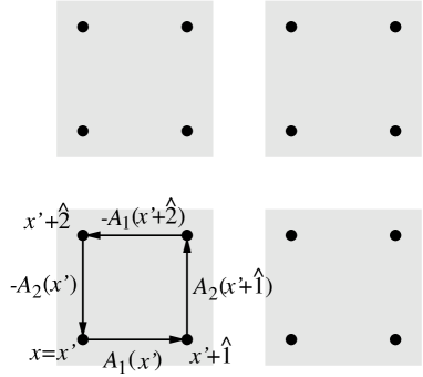
Figure 1: In the fine gauge the plaquette field strength within each block is distributed equally among the four link variables.

To get a well defined path integral in the BST and to apply our method we have to get rid of these fine gauge degrees of freedom. For that reason we integrate not over all gauge field configurations but only over those which are in the fine gauge.

$$\int D_{f}A\quad:=\int_{\begin{array}[]{c}\displaystyle A_{\mu}(x)\;\textrm{in}\cr\textrm{the fine gauge}\end{array}}DA\;.$$ (5)

The kernel of the BST for the fermions was taken from [8, 14],

$$\begin{array}[]{l}\displaystyle T(\bar{\Psi},\Psi,\bar{\Psi}^{\prime},\Psi^{\prime})=\\ \displaystyle\quad\quad\quad\frac{1}{a_{2}}\,\sum_{x^{\prime},i}\left(\bar{\Psi}^{\prime}_{i}(x^{\prime})-\frac{b_{2}}{4}\,\sum_{x\in x^{\prime}}\bar{\Psi}_{i}(x)\right)\left(\Psi^{\prime}_{i}(x^{\prime})-\frac{b_{2}}{4}\,\sum_{x\in x^{\prime}}\Psi_{i}(x)\right)\;,\end{array}$$ (6)

where one has has to choose $b_{2}=\sqrt{2}$ in order to have a fixed point for this BST and $a_{2}=1/4$ for maximum locality in the situation of free fermions. Here $\sum_{x\in x^{\prime}}$ denotes the sum over all fine lattice sites $x$ belonging to the coarse lattice site $x^{\prime}$.

For the kernel of the gauge field we define an average over the four 2-link connections between corresponding sites in adjacent blocks,

$$B_{\mu}^{\prime}(x^{\prime})=\frac{\beta_{2}}{8}\,\sum_{x\in x^{\prime}}\left(A_{\mu}(x)+A_{\mu}(x+\hat{\mu})\right)\;.$$ (7)

A lattice differential operator of second order may be defined as

$$\Delta_{\mu}B_{\nu}^{\prime}(x^{\prime})=\delta_{\mu\nu}\left(2B_{\mu}^{\prime}(x^{\prime})-B_{\mu}^{\prime}(x^{\prime}-2\hat{\mu})-B_{\mu}^{\prime}(x^{\prime}+2\hat{\mu})\right)\;.$$ (8)

With these conventions we write the BST for the gauge fields as follows:

$$T(A,A^{\prime})=\frac{1}{2}\sum_{x^{\prime},\mu}\left(A^{\prime}_{\mu}(x^{\prime})-B_{\mu}^{\prime}(x^{\prime})\right)(\alpha_{2}+\gamma_{2}\Delta_{\mu})^{-1}\left(A^{\prime}_{\mu}(x^{\prime})-B_{\mu}^{\prime}(x^{\prime})\right)\;.$$ (9)

For the wave function renormalization factor $\beta_{2}$, we choose the value 2 (as in the compact case of [8]) in order to make the action on the coarse lattice gauge invariant. This value is different from the one which would follow due to dimensional considerations and, in fact, for $\beta_{2}=2$ there exists only a quasi-FP for the BST of the gauge field. For this value of $\beta_{2}$ for ultra-locality one has to choose $\alpha_{2}=1/2$ and $\gamma_{2}=-1/32$.

With these values the BST respects the basic symmetries of the Schwinger model with Wilson fermions. The resulting action on the coarse lattice is gauge invariant, hermitian invariant, invariant under the charge conjugation and respects the lattice symmetry. It does violate chiral symmetry.

For given $A^{\prime}$ there exists a unique minimizing configuration of $S(A)+T(A,A^{\prime})$ which we denote by $A_{\textrm{\scriptsize min}}(A^{\prime})$. Since we use a non-compact gauge field with action and BST quadratic in the fields, $A_{\textrm{\scriptsize min}}(A^{\prime})$ can be computed straightforwardly by solving a set of linear equations. For $\beta\to\infty$ the saddle point $A_{\textrm{\scriptsize min}}(A^{\prime})$ dominates the path integral of the gauge field giving

$$\begin{array}[]{l}\displaystyle e^{-\beta^{\prime}S^{\prime}(A^{\prime})+S^{\prime}(\bar{\Psi}^{\prime},\Psi^{\prime},A^{\prime})+c}=e^{-\beta\left(S(A_{\textrm{\scriptsize min}})+T(A_{\textrm{\scriptsize min}},A^{\prime})\right)+c_{1}}\times\\ \displaystyle\times\left(\int D\Psi D\bar{\Psi}\,\exp\left[S(\bar{\Psi},\Psi,A_{\textrm{\scriptsize min}})+T(\bar{\Psi},\Psi,\bar{\Psi}^{\prime},\Psi^{\prime})\right]+{\cal O}\left(\frac{1}{\beta}\right)\right)\;,\end{array}$$ (10)

where $c_{1}$ is some constant which may be absorbed into $c$. For Grassmann variables the “gaussian” integral results in the exponential of an element of the Grassmann algebra in $\Psi^{\prime}$ and $\bar{\Psi}^{\prime}$. This algebra element is a sum of bilinear terms in the fermionic variables plus a constant. It may therefore be identified with the blocked fermionic action by determining the coefficients of the corresponding fermion matrix. Formally this is equivalent to the saddle point minimization for the bosonic action. Due to this analogy to bosons we will denote this process of integration over the Grassmann fields and subsequent identifications of the coefficient of the fermionic action by $\min_{\{\bar{\Psi},\Psi\}}$.

Having solved the two path integrals (the bosonic and the formal fermionic one) we separate the resulting action of (i.e. the logarithm of (10)) into two parts, one belonging to the scalar subspace of the Grassmann-algebra, the other one quadratic in the fermionic fields.

$$\beta^{\prime}S^{\prime}(A^{\prime}) = \beta\left(S(A_{\textrm{\scriptsize min}})+T(A_{\textrm{\scriptsize min}},A^{\prime})\right)+c_{2}(A_{\textrm{\scriptsize min}})+{\cal O}\left(\frac{1}{\beta}\right)\;,$$

$$S^{\prime}(\bar{\Psi}^{\prime},\Psi^{\prime},A^{\prime}) = \min_{\{\bar{\Psi},\Psi\}}\left(S(\bar{\Psi},\Psi,A_{\textrm{\scriptsize min}})+T(\bar{\Psi},\Psi,\bar{\Psi}^{\prime},\Psi^{\prime})\right)+{\cal O}\left(\frac{1}{\beta}\right)\;.$$ (11)

The constant $c_{2}(A_{\textrm{\scriptsize min}})$ is just the logarithm of the fermionic determinant resulting from the Grassmann integral. Compared to the leading term proportional to $\beta$ we may neglect this contribution and find that the fermions decouple completely from the gauge field BST. The defining equations for the FP-action finally have the form

$$\beta^{\prime}S_{*}(A^{\prime}) =\beta\,\min_{A\;\textrm{in the fine gauge}}\left(S_{*}(A)+T(A,A^{\prime})\right)\;,$$ (12)

$$S_{*}(\bar{\Psi}^{\prime},\Psi^{\prime},A^{\prime}) =\min_{\{\bar{\Psi},\Psi\}}\left(S_{*}(\bar{\Psi},\Psi,A_{\textrm{\scriptsize min}})+T(\bar{\Psi},\Psi,\bar{\Psi}^{\prime},\Psi^{\prime})\right)\;.$$ (13)

These equations replace now the BST at $\beta\to\infty$. Since we want to use the action also at moderate $\beta$ values, we have to calculate $S^{\prime}$ for strongly fluctuating configurations $A^{\prime}$, too. This however is naturally possible, since we never demanded that $A^{\prime}$ ought to be small. As was already mentioned in [5] this method has nothing to do with perturbation theory. It can be shown that the form of the action is independent of the number of fermion species.

Here we should mention that both, the FP-action for the gauge field and the FP-action for the fermions do have scale invariant solutions. For the gauge-field this was proven in [5]; for a non-compact gauge theory with periodic boundary conditions this is not very interesting, since there are no instanton solutions. For the fermionic FP-action the theorem takes the following form. Suppose that $\bar{\Psi}^{\prime}$ and $\Psi^{\prime}$ are solutions of the classical equations of motion $\partial S(\bar{\Psi}^{\prime},\bar{\Psi},A^{\prime})/\partial\bar{\Psi}^{\prime}=0$ and $\partial S(\bar{\Psi}^{\prime},\bar{\Psi},A^{\prime})/\partial\Psi^{\prime}=0$, i.e. are part of the null-space of the fermionic matrix, then also the minimizing configurations of (13) $\bar{\Psi},\Psi$ on the fine lattice are solutions of the equations of motion corresponding to $S(\bar{\Psi},\Psi,A_{\textrm{\scriptsize min}}(A^{\prime}))$.

In the following two sections we discuss how to solve (12) by analytical methods and (13) by numerical methods.

2.1 The FP-action for the gauge field

For details we refer to [14, 8]. For our choice of the parameters of the BST the ultra-local standard (non-compact) plaquette action is a fixed point, up to the wave function renormalization. In $d=2$ this action is

$$S_{P}(A) = \frac{1}{2}\,\sum_{x}F(x)^{2}$$ (14)

$$= \frac{1}{2}\,\sum_{x}\left(A_{2}(x+\hat{1})-A_{2}(x)-A_{1}(x+\hat{2})+A_{1}(x)\right)^{2}\;.$$

As it was shown in [8] on an infinite lattice the equation

$$\frac{1}{4}S_{P}(A^{\prime})=\min_{\{A\}}\left(S_{P}(A)+T(A,A^{\prime})\right)$$ (15)

is valid. It is remarkable, that (15) is also exactly fulfilled on a finite lattice as long as $S_{P}$ fits on the coarse lattice. For this reason we forget about the finite size effects even in the case of the FP-action for the fermions (cf. also [18]).

Although $S_{P}$ is strictly speaking not a fixed point under the BST (due to the necessary but trivial rescaling of $\beta$) it is still a perfect action. In the Schwinger model it is classically perfect and for the free gauge field it is quantum perfect, since it describes the same physics as on an infinite fine lattice. To determine the FP-action for the fermions it is necessary to iterate the BST and therefore it is necessary to renormalize $\beta^{\prime}\to 4\beta$ after each step to avoid the unwanted convergence of $\beta\to 0$.

2.2 The FP-action for the fermions

The fixed point action for the fermions can be calculated in a perturbation expansion as was shown in [8, 14] or more explicitly in [17]. But in [19] the authors demonstrate for the case of the Gross-Neveu model at large $N$ that the non-perturbative approach of [5] is really necessary to calculate the perfect action.

Eq. (13) defines the action on the coarse lattice for any configuration $A^{\prime}$, and – as we discuss later – one can advise numerical procedures which calculate the action to high precision. However, since we want to iterate the BST and since we want to use this action in numerical simulations we have to parameterize $S^{\prime}(\bar{\Psi}^{\prime},\Psi^{\prime},A^{\prime})$ with a finite number of coupling constants.

$$S_{F}(\bar{\Psi},\Psi,A)=\bar{\Psi}M_{F}(A)\Psi=\sum_{i=0}^{3}\sum_{x\,,f}\,\rho_{i}(f)\,\bar{\Psi}(x)\sigma_{i}U(x,f)\Psi(x+\delta f)\;.$$ (16)

Here $M_{F}(A)$ is the parameterized fermion matrix. By $f$ we denote a closed loop through $x$ or a path from the lattice site $x$ to $x+\delta f$ ($\delta f$ denotes the distance vector on the lattice corresponding to the path $f$). $U(x,f)$ is the parallel transporter (i.e. the element of the compact group) along this path. The $\sigma_{i}$-matrices denote the Pauli matrices for $i=1,2,3$ and the $2\times 2$ unit matrix for $i=0$.

We have to ensure that the BST stays on the critical surface and eventually converges to the nontrivial fixed point. Thus we impose the condition

$$\sum_{f}\rho_{0}(f)=0\;,$$ (17)

which guarantees, that $S_{F}$ reproduces the action of the massless continuum Schwinger model in the naive continuum limit. The normalization of $\rho$ is fixed by demanding

$$\sum_{f}\rho_{1}(f)(\delta f)_{1}=1\;.$$ (18)

Here $(\delta f)_{1}$ denotes the component of the path vector in the 1-direction. We want to emphasize that (16) is not the most general parameterization. E.g., since the gauge fields enter as parallel transporter in their compact version a clover-term $\bar{\Psi}(x)F_{\mu\nu}(x)\Psi(x)$, which contains the non-compact field strength, can be represented only in an approximate way for values $-\pi<F(x)<\pi$. For sufficiently large values of $\beta$ this should be no problem.

We require the invariance of the action under certain symmetries; thus we can impose some conditions for the coupling constants $\rho_{i}(f)$. For example hermitian invariance and invariance under charge conjugation implies that $\rho_{0,1,2}(f)$ has to be real and $\rho_{3}(f)$ has to be purely imaginary. These and further symmetries due to the lattice geometry drastically reduce the number of independent coupling constants. We have considered terms that connect the central site $x$ with any other site $x+\delta f$ in a $7\times 7$ lattice. Concerning the length of the connecting paths $f$ we first considered paths which may exceed the shortest connection between $x$ and $x+\delta f$ by up to 8 links and some extra paths containing higher powers of plaquette variables. However, in the iteration procedure it turned that one may omit many of these. Altogether, respecting the mentioned symmetries, we finally considered 33 different geometric shapes corresponding to 123 independent coupling constants [20].

For the determination of the fixed point action we proceed as follows. The starting point for the fermionic action is the Wilson action for the massless Schwinger model ($\kappa=1/4$).

1. We generated 50 gauge field configurations $A^{\prime}$ on the coarse $7\times 7$ lattice according to their probability distribution $e^{-\beta^{\prime}S_{P}(A^{\prime})}$ (with periodic boundary conditions). For definiteness this has to be done in a fixed gauge. Technically, we do this by randomly sampling the non-zero diagonal elements of the momentum space representation of the action [21]. For each of these configurations we then calculate the corresponding minimizing configuration $A_{\textrm{\scriptsize min}}(A^{\prime})$ as described above.

2. With the help of $A_{\textrm{\scriptsize min}}(A^{\prime})$ we generate the fermion matrix on the fine lattice and performed the BST (Grassmann integral) for the fermions giving the $(2\cdot 7^{2})\times(2\cdot 7^{2})$ fermion matrix $M_{BST}(A_{\textrm{\scriptsize min}})$ on the coarse lattice. This is done for all 50 gauge field configurations.

3. The resulting fermion matrices are then compared with the fermion matrices $M_{F}(A^{\prime})$ for the coarse lattice generated for the corresponding $A^{\prime}$ configurations. A new set of parameters according (16) is now determined by minimizing

   $$\sum_{A^{\prime}}\|M_{BST}\left(A_{\textrm{\scriptsize min}}(A^{\prime})\right)-M_{F}(A^{\prime})\|^{2}\;,$$ (19)

   where the matrix norm is defined

   $$\|M\|^{2}\equiv\sum_{i,j}\,|M_{ij}|^{2}\>.$$ (20)

All these steps are iterated until the coupling constants remain stable within small statistical fluctuations.

We worked at $\beta^{\prime}=20$ which corresponds to a typical value for the field strength $F(x)\approx 0.18$. After ${\cal O}(10)$ iterations the coupling constants stabilized and subsequent iterations stayed within the statistical errors. The largest matrix element is $\sim 1.4$; the average deviation between individual matrix elements given by the BST and by the parameterization was $0.00024$ in the last iteration step. Comparing different sets of $A^{\prime}$ the values of the coupling constants we obtained in this way differed in the mean by $0.0017$, which provides an estimate of the possible systematic uncertainty due to the finite number of configurations. We have no control on possible redundancies in the parameterized action. Thus it may well be, that part of the observed (small) fluctuations in the couplings is due to cancellations of certain terms in the fermionic action. The final action therefore may have been determined to an even higher accuracy.

Figure 2: (a) Symbolic representation of some of the $\sigma_{3}$ couplings of the perfect action. Crosses and circles mark the position of the $\bar{\Psi}$ and $\Psi$. Each block of arrows corresponds to a term $\rho_{3}(f)\,\bar{\Psi}(x)\,\sigma_{3}\,U(x,f)\,\Psi(x+\delta f)$, where $f$ is symbolized by arrows and the coupling $\rho_{3}(f)$ is written at the height of the arrows. (b) Terms building the perfect clover term.

In figure 2 we show a subset of the couplings of the FP-action, which is proportional to $\bar{\Psi}\sigma_{3}\Psi$. In the limit of small $A_{\mu}(x)$ one can expand $U(x,f)$ and the expressions linear in $A_{\mu}(x)$ can be compared with Fig. 14 of [17]. If we compare the two most important operators of this perfect clover term, our result agrees within a few percent with [17]. The smaller coupling constants of the clover term have already rather large statistical errors. The locality of our FP-action is established by comparing our couplings with the situation of vanishing gauge fields. We find that our values are similar or smaller than those obtained for the free fermion perfect action [8]. The complete set of couplings may be retrieved from [20].

3 Simulation of the FP-action

For notational simplicity we call now the obtained parameterization of the FP-action just the FP-action. For $\beta\to\infty$ the FP-action is on the RT by construction. For finite values of $\beta$ it may be no longer perfect. This depends on the system considered; the FP-action of the O(3)-model turned out to stay close to perfectness [5]. In order to check the amount of improvement, we have to rely on direct simulations with the FP-action. Indeed, as will be shown below, we found significant improvement for all observables studied.

One has to determine the path integral

$$\frac{1}{Z}\int DA\,\int D\Psi D\bar{\Psi}\,{\cal{O}}(\bar{\Psi},\Psi,A)e^{-\beta S_{P}(A)+S(\bar{\Psi},\Psi,A)}\;.$$ (21)

A full-scale (hybrid-) Monte-Carlo simulation for the FP-action is a highly non-trivial task. We decided to work on lattices of moderate size up to $16\times 16$. In this case one may perform the Grassmann integrals explicitly, i.e. by computing the corresponding determinant and inverse fermion matrix.

For a simulation we generated $5000$ gauge field configurations with periodic boundary conditions according to their gaussian probability distribution $e^{-\beta S_{P}(A)}$ with gauge fixing as has been discussed above in Sec. 2.2 in the context of the BST. For these configurations we determined the fermionic path integral as discussed with standard routines of linear algebra.

The side-benefit of this approach is that we obtain results for both, the determinant corresponding to the 1-flavour model and its square, corresponding to the 2-flavour situation. All observables are obtained in that way. In order to estimate the statistical errors we repeated the whole procedure several times (several runs of 5000 gauge configurations each). We compared the results obtained with the FP-action with results obtained in in the same way for the Wilson-action for fermions (but still using the non-compact form of the gauge field action). For the Wilson action we use $\kappa=0.25$ throughout. This is below the critical value $\kappa_{c}(\beta)$ which, however, approaches 0.25 asymptotically. We therefore do not expect perfect agreement of the obtained physical mass values for thw Wilson action. However, for a qualitative comparison of improvement properties this choice should be sufficient.

Figure 3: Improvement of rotational invariancefor the correlation function (22) in the 1-flavour model for (left-hand plot) Wilson and (right-hand plot) the FP-action on a $16\times 16$ lattice at $\beta=6$.

Fig. 3 exhibits for the 1-flavour model the correlation function

$$P(x)=\langle\bar{\Psi}(0)\,\sigma_{3}\,\Psi(0)\,\bar{\Psi}(x)\,\sigma_{3}\,\Psi(x)\rangle$$ (22)

measured for all 2-point separations. The numbers have been determined at $\beta=6$. One finds much better rotational invariance for the FP-action than for the Wilson-action.

Figure 4: Dispersion relation of the massive boson in the 1-flavour Schwinger model with Wilson fermions (diamonds) and with the FP-action (full circles) calculated on a $16\times 16$ lattice at $\beta=6$, compared with the continuum dispersion relation $E(p)=\sqrt{m^{2}+p^{2}}$.

Figure 5: Dispersion relation of the massless ($\pi$) boson in the 2-flavour Schwinger model with the FP-action calculated on a $16\times 16$ lattice at $\beta=6$, compared with the continuum dispersion relation $E(p)=p$.

In the 2-flavour Schwinger model one expects one massive mode (which we call $\eta$ by analogy) and a massless flavour-triplet (called $\pi$). The corresponding momentum-projected operators are

$$\eta(p,t) = \sum_{x_{1}}\,e^{ipx_{1}}\left(\bar{u}(x_{1},t)\,\sigma_{1}\,u(x_{1},t)+\bar{d}(x_{1},t)\,\sigma_{1}\,d(x_{1},t)\right)\;,$$ (23)

$$\pi(p,t) = \sum_{x_{1}}\,e^{ipx_{1}}\left(\bar{u}(x_{1},t)\,\sigma_{1}\,u(x_{1},t)-\bar{d}(x_{1},t)\,\sigma_{1}\,d(x_{1},t)\right)\;.$$ (24)

Their correlation functions define by their exponential decay the corresponding energy functions $E(p)$. In Fig.4 we present results for the $\eta$ dispersion relation for the Wilson-action and the FP-action and compare these with the continuum dispersion relation. Again we find significant improvement.

Figure 6: Masses for the massive (full circles) and the massless (diamonds) modes in the 2-flavour Schwinger model vs. $1/\sqrt{\beta}$; the values have been determined with the FP-action on an $16\times 16$ lattice. The line denotes the theoretical expectations for scaling.

The dispersion relation for the $\pi$-state is plotted in Fig. 5 only for the FP-action. For the Wilson action at $\kappa=0.25$ and $\beta=6$ this state has a non-vanishing mass and is therefore not suitable for a comparison.

It is remarkable that the $\pi$-mass obtained by the means of the FP-action is even numerically very close to zero (e.g. 0.005 at $\beta=6$), whereas with Wilson-fermions one has to search for a critical point in $\kappa$. In fact for $\beta\to\infty$ this constitutes a test for the perfectness of the FP-action, since for the optimal action of course one has to recover the massless continuum Schwinger model properties. Also the masses obtained for the massive mode are within the statistical errors in agreement with the theoretical expectations, e.g. $m_{\eta}=0.33(1)$ compared to 0.3257 from continuum theory (at $\beta=1/g^{2}=6$). Since the mass from the lattice propagator has been determined by the usual $\cosh$-fit on $16\times 16$ lattices the value has to be handled with some caution.

Fig. 6 shows the obtained masses for massive and massless modes at various values of $\beta$ (determined with the FP-action on $16\times 16$-lattices). We find clear signals of non-vanishing $\pi$-masses at sufficiently small $\beta$, indicating deviation of our FP-action from the renormalized trajectory. However, the overall scaling behaviour predicted (for the 2-flavour model) from theory,

$$a(\beta)\,m_{\eta}=\sqrt{\frac{2}{\pi\,\beta}}\;$$ (25)

is nicely recovered for moderately large values of $\beta>3$.

4 Conclusion

For the 2D Schwinger model we determined the optimal FP-action for interacting fermions in a non-perturbative background of gauge fields. The parameterized action contains 123 independent couplings localized in a $7\times 7$ lattice centered around one of the fermionic fields.

With this action we have simulated the model on a $16\times 16$ lattice for various values of the gauge coupling and for one and two species of fermions. Our results show excellent improvement of the important propagator observables, although we did not improve those operators.
 
Acknowledgment: We wish to thank W. Bietenholz, F. Farchioni, I. Hip, U.-J. Wiese and E. Seiler for discussions.

References

- [1] K. Symanzik, Nucl. Phys. B 226 (1983) 187.
- [2] B. Sheikholeslami and R. Wohlert, Nucl. Phys. B. 259 (1985) 572.
- [3] K. Jansen et al., Phys. Lett. B 372 (1996) 275.
- [4] G. P. Lepage and P. B. Mackenzie, Phys. Rev. D 48 (1993) 2250.
- [5] P. Hasenfratz and F. Niedermayer, Nucl. Phys. B 414 (1994) 785.
- [6] T. Bell and K. Wilson, Phys. Rev. B 10 (1974) 3935.
- [7] U.-J. Wiese, Phys. Lett. B 315 (1993) 417.
- [8] W. Bietenholz and U.-J. Wiese, Nucl. Phys. B 464 (1996) 319.
- [9] U. Kerres, G. Mack, and G.Palma, Nucl. Phys. B 467 (1996) 510.
- [10] F. Niedermayer, Nucl. Phys. B (Proc. Suppl.) 53 (1997) 56.
- [11] T. DeGrand, A. Hasenfratz, P. Hasenfratz, and F. Niedermayer, Nucl. Phys. B 454 (1995) 587.
- [12] F. Farchioni, P. Hasenfratz, F. Niedermayer, and A. Papa, Nucl. Phys. B 454 (1995) 638.
- [13] P. Hasenfratz and F. Niedermayer, Fixed-point actions in 1-loop perturbation theory, BUTP/97-13,hep-lat/9706002, 1997.
- [14] W. Bietenholz and U.-J. Wiese, Phys. Lett. B 378 (1996) 222.
- [15] F. Farchioni and V. Laliena, private communication.
- [16] J. Schwinger, Phys. Rev. 128 (1962) 2425.
- [17] W. Bietenholz, R. Brower, S. Chandrasekharan, and U.-J. Wiese, Nucl. Phys. B (Proc. Suppl.) 53 (1997) 56.
- [18] T. DeGrand, A. Hasenfratz, P. Hasenfratz, and F. Niedermayer, Nucl. Phys. B 454 (1995) 615.
- [19] W. Bietenholz, E. Focht, and U.-J. Wiese, Nucl. Phys. B 436 (1995) 385.
- [20] WWW URL http://physik.kfunigraz.ac.at/cbl/cbl-pa-couplings.html
- [21] J. Challifour and D. Weingarten, Ann. Phys. (N.Y.) 123 (1979) 61.