CERN-TH/97-160

July 1997

Two-Cutoff Lattice Regularization of Chiral Gauge Theories

P. Hernández

Theory Division, CERN

CH-1211 Geneva 23, Switzerland

I review our method to formulate chiral gauge theories on the lattice based on a two-cutoff lattice regularization and discuss recent numerical results in a chiral $U(1)$ gauge theory in 2D.

1 Introduction

The well-known theorem by Nielsen and Ninomiya (NN) sets very strong constraints on the possibility of constructing a non-perturbative regulator with an exact chiral symmetry. On the lattice, the difficulty is related to the presence of doubler modes, which render any symmetric discretization of a chiral theory effectively vector-like. The doublers can be given masses of the order of the cutoff, and thus be decoupled in the continuum limit, but only at the expense of explicitly breaking the chiral symmetry. In the case of a chiral gauge theory, this implies the explicit breaking of the gauge symmetry and it is highly non-trivial to ensure that, in the continuum limit, the gauge symmetry is restored, without changing the particle content of the model. The Roma approach [1] addresses this issue and provides a solution based on a non-perturbative tuning of all dimension-four or less counterterms, necessary to ensure that BRST identities, which are broken at the regulator level, are satisfied in the continuum limit. Although the validity of this method is expected to hold to all orders in perturbation theory, its practicability in real simulations is questionable.

I will review here an alternative method that we recently proposed [2, 3] to deal with chirality on the lattice. Our formulation of chiral gauge theories involves two essential ingredients.

Small breaking of gauge invariance at the cutoff level. Even though the gauge symmetry has to be broken at the cutoff level, according to NN, it is still possible to constrain this breaking to be arbitrarily small. This is achieved by using a two-cutoff (TC) lattice formulation [2], in which the fermion momenta are cut off at a scale much larger than the boson momenta. More explicitly, the fermions live on a lattice of spacing $f$ and are coupled to gauge link variables that are constructed by an appropriate smooth and gauge-invariant interpolation of gauge configurations [4][3] that are generated on a coarser lattice of spacing $b$. As long as the interpolation is smooth, the Fourier modes of the interpolated field are effectively cut off at the scale $1/b\ll 1/f$. Doublers are decoupled by introducing a naive Wilson term as in the Roma approach [1]. However, the chirally breaking effects due to the Wilson term are relevant only at scales of the order of the fermion cutoff (the Wilson term is a higher-dimensional operator suppressed by the fermion cutoff), and gauge boson momenta are not large enough to prove these interactions, in contrast with one-cutoff (OC) formulations. As a result, due to the separation of the cutoff scales, it can be shown that no fine-tuning is necessary to recover an approximate chiral (global or gauge) symmetry. The parameter $f/b$, which can be chosen to be arbitrarily small in principle, controls the strength of the breaking of chirality. It is important to stress that this is not true if there are gauge anomalies. If the theory is anomalous fermion loops induce gauge-breaking effects of $O(1)$ that cannot be subtracted. No approximate gauge invariance is possible in this case. In section 2, we will review the details of our two-cutoff formulation.

The Foester, Nielsen and Ninomiya (FNN) mechanism of dynamical restoration at large distances of a lattice gauge symmetry that is mildly broken at short distances [5]. Even though the two-cutoff construction will have an approximate gauge invariance, in any real simulation the ratio $f/b$ will be finite. In this situation there is always some residual breaking of gauge invariance and it is then essential that the lattice model at finite $f/b$ be in the same universality class as the model with $f/b=0$ . In section 3, we will review the FNN mechanism and extend the reasoning to the particular case of chiral gauge theories.

In section 4, we will present the first numerical test of the TC method in a simple $U(1)$ chiral model in 2D.

2 Two-Cutoff Lattice Formulation

In [2] and [3], we presented a two-cutoff lattice construction of chiral gauge theories. Two different proposals with a similar philosophy were given in [6, 7]. Another earlier idea, in which fermions regulated in the continuum are coupled to interpolated lattice gauge fields [8], might also lead naturally to a TC construction.

The advantage of using two-cutoffs, as we have explained, is precisely to make the violations of gauge invariance small. With one-cutoff a non-perturbative tuning of counterterms would be needed to achieve this [1]. The way in which the cutoff separation is implemented is by the use of two lattices. The gauge degrees of freedom are the Wilson link variables of a Euclidean lattice of spacing $b$, ${\cal L}_{b}$. We will call $s$ the sites of the $b$-lattice. The gauge action is the standard one:

$$S_{g}=\frac{2}{g^{2}}\sum_{s}\sum_{\mu<\nu}[I-\frac{1}{2}(U_{\mu\nu}+U_{\mu\nu}^{\dagger})]$$

$$U_{\mu\nu}\equiv U_{\mu}(s)U_{\nu}(s+\hat{\mu})U_{\mu}^{-1}(s+\hat{\nu})U_{\nu}^{-1}(s).$$ (1)

Fermions on the other hand live on the sites of a finer lattice ${\cal L}_{f}$ (some integer subdivision of ${\cal L}_{b}$). We refer to the $f$-lattice sites as $x$. In order to decouple the unavoidable doublers, a Wilson term is included in the fermionic action. For each charged chiral fermion, a singlet of the opposite chirality is needed. The fermions are coupled to the gauge fields through a standard lattice gauge–fermion coupling on the $f$-lattice. The link variables on ${\cal L_{f}}$ are obtained through a careful interpolation of the real dynamical fields, i.e. $U_{\mu}(s)$. As long as the interpolation is smooth, it is clear that the separation of scales is achieved in this construction, since the high-momentum modes of the gauge fields are cut off at the scale $b^{-1}$, while the fermions can have momenta of $O(f^{-1})$. The lattice action for a charged left-handed fermion field is then given by

$${\cal L}_{fermion} = \frac{1}{2}\sum_{\mu}\bar{\Psi}\gamma_{\mu}[(D^{+}_{\mu}+D_{\mu}^{-})P_{L}+(\partial^{+}_{\mu}+\partial^{-}_{\mu})P_{R}]\Psi$$ (2)

$$+ y\;\bar{\Psi}\Psi-\frac{r}{2}\bar{\Psi}\sum^{d}_{\mu=1}\partial_{\mu}^{+}\partial^{-}_{\mu}\Psi\equiv\bar{\Psi}\;{\hat{D}}\;\Psi,$$

where the covariant and normal derivatives are given by $D_{\mu}^{+}\Psi(x)=u_{\mu}(x)\Psi(x+\hat{\mu})-\Psi(x)$, $D_{\mu}^{-}\Psi(x)=\Psi(x)-u^{\dagger}_{\mu}(x-\hat{\mu})\Psi(x-\hat{\mu})$, $\partial_{\mu}^{+}=D_{\mu}^{+}|_{u=1}$ and $\partial_{\mu}^{-}=D_{\mu}^{-}|_{u=1}$ and we have introduced a bare mass term for later use. As explained above, the $u_{\mu}(x)$ link variables are interpolations of the real dynamical fields $U_{\mu}(s)$. When we refer to $f$-lattice quantities we use $f=1$ units and when we refer to $b$-lattice quantities we use $b=1$ units for notational simplicity. This should create no confusion.

The TC lattice path integral is defined to be

$$Z=\int_{{\cal L}_{b}}{\cal D}U\;\;\;e^{-S_{g}[U]}\;\;e^{\Gamma[u[U]]}\;\;e^{-\bar{\eta}\;G[u[U]]\;\eta},$$ (3)

where ${\cal D}U$ is the standard $b$-lattice gauge measure, $G[u[U]]\equiv\hat{D}^{-1}$, and we define $\Gamma[u[U]]$ in the following way:

$$\Gamma[u[U]]\equiv Phase({\det}_{f}(\hat{D}))\;\;\sqrt{{\det}_{f}(\not\!\!D)},$$ (4)

where $\not\!\!D$ is the standard Wilson-Dirac operator on the $f$-lattice (i.e. the naive Dirac operator plus a covariant Wilson term). The reason for this choice as opposed to the obvious one, i.e. $\Gamma[u[U]]=\det_{f}(\hat{D})$, is that in this way there is no breaking of gauge invariance in the real part of the effective action. This definition is justified from the equivalent formal relation between the corresponding continuum operators [9]. If the real part broke gauge invariance, then it would be necessary to subtract several gauge non-invariant local counterterms generated by fermions at one loop [2]. Even though, in the TC method, only a one-loop subtraction would be needed (as opposed to the non-perturbative tuning required in the Roma approach), it is nevertheless a more difficult procedure , and thus we prefer the choice (4), where no subtraction is needed.

It was shown in [2] that, at the one-loop level, under an infinitesimal gauge transformation $\omega$ on the $f$-lattice,

$$\delta_{\omega}\Gamma[u]=Consistent\;Anomaly+O(f^{2}).$$ (5)

Thus if gauge anomalies cancel, as we will assume the case to be, the fermionic effective action is gauge-invariant up to irrelevant terms. Now, the power of the TC method is that these terms, which in OC constructions would induce $O(1)$ effects at higher orders, in this case become at most $O(f/b)^{2}$ to all orders, because gauge boson integration cannot bring back powers of $1/f$, but only $1/b$. In order to prove this statement, we have to be more explicit about the interpolated field, $u_{\mu}(x)$, which is a complicated function of the $b$-lattice gauge fields $U_{\mu}(s)$.

For a detailed explanation of how to construct such an interpolation for the general case of a non-Abelian gauge theory in 4D, the reader is refered to [3]. I just list here the properties that this interpolation must satisfy in order to achieve the cutoff separation.

• The interpolation is of course gauge-covariant under gauge transformations on the $b$-lattice, i.e. there exists a gauge transformation on the $f$-lattice, $\omega(x)$, such that

  $$u_{\mu}[U^{\Omega}](x)=\omega(x)\;u_{\mu}[U](x)\;\omega^{\dagger}(x+\hat{\mu})\equiv u_{\mu}^{\omega}(x).$$ (6)

  In this way, any functional that is gauge-invariant on the $f$-lattice is automatically gauge-invariant under the $b$-lattice gauge transformations (notice that the relevant gauge symmetry is that on the $b$-lattice).

• The interpolation must be covariant under the remaining discrete $b$-lattice symmetries ($90^{\circ}$ rotations, translations, spatial and temporal inversions). This is important to ensure that Lorentz symmetry is recovered in the continuum limit $b\rightarrow 0$.

• The interpolation has to be smooth in order to achieve the cutoff separation. In [2], it was shown that a sufficient condition to ensure that the gauge symmetry violations induced by the Wilson term in (4) are suppressed by $O(f/b)$ is that the interpolated field, in the limit $f\rightarrow 0$, describes a differentiable continuum gauge field inside each $b$-lattice hypercube, and its transverse components are continuous across hypercube boundaries. We refer to this property as transverse continuity. From it, one can easily deduce a bound on the high Fourier modes of the interpolated field,

  $$|a_{\mu}(q)|\leq\frac{C}{|q_{\mu}|}\prod_{\alpha\neq\mu}\frac{1}{q_{\alpha}^{2}}$$ (7)

  where $C$ is independent of $f$ and $u_{\mu}\equiv e^{ia_{\mu}f}$. Using this bound it can be shown that

  $$\Gamma[u[U^{\Omega}]]-\Gamma[u[U]]=O(f/b)^{2}$$

  $$G[u[U^{\Omega}]]-G[u[U]]=O(f/b)^{2},$$ (8)

  where $\Omega$ is a $b$-lattice gauge transformation and, in the second equation, we have assumed that the external fermion momentum is smaller than $O(1/b)$. The proof in [2] is just based on the derivation of bounds for the lattice integrals corresponding to all the terms in the perturbative expansions of $\Gamma[u[U^{\Omega}]]-\Gamma[u[U]]$ and $G[u[U^{\Omega}]]-G[u[U]]$.

• The gauge-invariant degrees of freedom of the interpolated field should be local functions of those of $U_{\mu}$, where by local we mean within distances of $O(b)$. The reason for this is clear. If the gauge-invariant degrees of freedom of the interpolated fields were not constructed locally from the $U{\mu}$, the interpolation could modify the non-local properties of the correlation functions of gauge-invariant quantities and thus the physics would be interpolation-dependent. What is not so obvious is whether the gauge-dependent degrees of freedom of the interpolated field should also be constructed locally from the $U_{\mu}$. The reason why this does not seem to be necessary is that, even if gauge-dependent degrees of freedom of $u_{\mu}$ were correlated at large distances with respect to $O(b)$ owing to the interpolation, this would at most induce long-range correlations suppressed by $O(f/b)^{2}$ in the physical sector, according to (8). We can then always choose the cutoff ratio to be as small as is necessary to ensure that these unphysical correlations are negligible (for instance at any finite volume, we can choose the cutoff ratio small enough so that the long-range correlation, induced by the non-locality of the interpolation, between two physical fields at points $x_{i}$ and $x_{j}$ is smaller than $\exp(-|x_{i}-x_{j}|/b)$). In general we expect that the less local the interpolation is, the smaller the cutoff ratio will have to be; so, for practical reasons, it would be much preferable that the interpolation be as local as possible. Our interpolation in [3] has the property that all gauge-invariant degrees of freedom of the interpolated field (for instance all the Wilson loops) depend on the $U_{\mu}$ strictly locally. However, this is not the case for the gauge-dependent degrees of freedom in $u_{\mu}$ [10]. In general it is expected that for any group $G$ in $d$ space-time dimensions, whenever any of the $\Pi_{n}(G)$ for $n\leq d-1$ is non-zero, the gauge-dependent degrees of freedom of the interpolated field is either singular or depends non-locally on the $U_{\mu}$ fields [3]. Our numerical results for $U(1)$ in 2D show, however, that the non-locality of the gauge-dependent degrees of freedom of $u_{\mu}$ is mild, in the sense that the correlation length of the $u_{\mu}$ fields, averaged over random $U_{\mu}$ configurations, is finite and of $O(b)$. However, we do not have a proof of this in the general case.

3 Effective Gauge Invariance

The TC formulation only ensures that there is an approximate gauge invariance for small $f/b$, but in any simulation this ratio is necessarily finite, so our lattice action is not gauge-invariant. There are, however, good arguments to believe that a pure gauge theory with a mild breaking of gauge invariance at short distances flows in the IR to a theory with an effective gauge symmetry and no extra light degrees of freedom. The argument of ref. [5] starts by showing that any lattice gauge theory (for a compact group) that contains some terms that break the lattice gauge invariance is equivalent to a theory with an exact gauge invariance and additional scalar degrees of freedom. This is simple to see. Let us consider a lattice action that contains gauge-breaking interactions:

$$S[U]=S_{g.i.}[U]+\delta S_{n.g.i.}[U].$$ (9)

The path integral is

$$Z=\int{\cal D}U_{\mu}\;\;e^{-S_{g.i}[U]-\delta S_{n.g.i.}[U]}.$$ (10)

Since the group is compact we can multiply $Z$ by the volume of the group $\int{\cal D}\Omega$, which is an irrelevant constant factor:

$$Z=\int{\cal D}\Omega\int{\cal D}U_{\mu}\;\;e^{S_{g.i}[U]+\delta S_{n.g.i.}[U]}.$$ (11)

Performing a change of variables from $U_{\mu}$ to $U^{\Omega}_{\mu}\equiv\Omega(x)U_{\mu}(x)\Omega^{\dagger}(x+\hat{\mu})$ (i.e. the gauge-transformed variables under the lattice gauge transformation $\Omega$), and using the invariance of the measure and $S_{g.i.}$ under a gauge transformation, we get

$$Z=\int{\cal D}\Omega\int{\cal D}U_{\mu}\;\;e^{S_{g.i}[U]+\delta S_{n.g.i.}[U^{\Omega}]}.$$ (12)

It is easy to see that (12) is gauge-invariant under a new gauge symmetry under which the field $\Omega$ transforms as

$$U_{\mu}(x) \rightarrow \Phi(x)U_{\mu}(x)\Phi^{\dagger}(x+\hat{\mu})\;\;\;\;\Omega(x)\rightarrow\Omega(x)\Phi(x)^{\dagger}.$$ (13)

This is because $U_{\mu}^{\Omega}$ is invariant under this transformation. This theory is then a gauge theory with extra charged scalars in a non-linear realization ($\Omega$ is unitary). These scalars are the pure gauge transformations, which couple through the non-invariant terms in the original action. It is clear that in any successful proposal for regulating chiral gauge theories, these scalars must decouple from the light physical spectrum. In the case of a spontaneously broken gauge theory these degrees of freedom remain, since they become the longitudinal gauge bosons.

The FNN conjecture is that (12) flows in the IR to the same point as the theory (10) with $\delta S_{n.g.i.}=0$, provided that the strength of the interactions in $\delta S_{n.g.i.}$ is “small”. Their argument is quite simple. Let us suppose that the characteristic coupling of the non-invariant terms is arbitrarily small at the cutoff scale. Then in the gauge-invariant picture of the theory (12), this implies that the $\Omega$ fields are very weakly coupled. Consequently, the free energy will be maximized when the $\Omega$ variables are decorrelated at distances of the order of the cutoff (i.e. the lattice spacing) or, in other words, these degrees of freedom are effectively very massive. Then it makes sense to integrate them out in order to obtain an effective theory at low energies. At distances larger than the lattice spacing, but still smaller than the correlation length of the gauge-invariant degrees of freedom, it can be argued that the effective action should be local, because the $\Omega$ integration does not generate long-range correlations, and exactly gauge-invariant. (It is clear from eq. (12) that if we perform the integration over $\Omega$, what remains is an exactly gauge-invariant theory due to the exact symmetry (13).) In this situation, the only effect of the $\Omega$ fields is a renormalization of the gauge-invariant couplings in $S_{g.i.}$.

In the case we are interested in, there are also fermions. The previous reasoning would imply that the IR limit of the model (3) would be equivalent to that of the original theory without a Wilson term (since this is the only term in $\delta S_{n.g.i.}$), and thus with doubling [11]. The reason why do not expect this to be the case in the TC formulation is that the $\Omega$ integration gives an action that is expected to be local at distances of $O(b)$, but not at distances of $O(f)$. This implies that after integrating the $\Omega$ fields, the effective fermion action on the $f$-lattice is not local. This is presumably how it can evade NN. On the other hand, if the $\Omega$ fields decouple at distances of $O(b)$, there must exist an effective action at the $b$-scale that involves only the light fermionic degrees of freedom and would be local and gauge-invariant. Of course, it should violate in some other way the conditions of the NN theorem. In particular, there is no reason to believe that it would be bilinear in the fermion fields. In this case, it would not be very useful in real simulations.

In any case, it is clear that in the presence of fermions, the decoupling of the $\Omega$ fields is not enough to ensure the right particle content. One should make sure that the light fermion spectrum after the $\Omega$ integration is the correct one. It is easy to show that also our TC formulation of (3) is equivalent to a new theory with additional scalar degrees of freedom and an exact gauge symmetry. We will call this reformulation the Wilson-Yukawa picture, for reasons that will become clear. Following the previous steps and using the property (6), the model (3) is exactly equivalent to

$$Z=\int_{{\cal L}_{b}}{\cal D}\Omega\;\int_{{\cal L}_{b}}{\cal D}U\;\;\;e^{-S_{g}[U]}\;\;e^{\Gamma[u^{\omega}[U]]}\;\;e^{-\bar{\eta}G[u^{\omega}[U]]\eta},$$ (14)

where the $\omega$ fields are defined by (6) and are coupled uniquely through the Wilson and mass terms. The $\omega$ fields are functions of the $\Omega$ and $U_{\mu}$ fields and the interpolation procedure, and can be interpreted as smooth interpolations of the $\Omega$ fields to the $f$-lattice. The transverse continuity property of the interpolation also implies that the $f\rightarrow 0$ limit of $\omega$ is a differentiable field inside each $b$-hypercube and continuous across $b$-boundaries [3]. Its high Fourier modes $q>b^{-1}$ are then strongly suppressed,

$$|\omega(q)|\leq\prod_{\mu}\frac{C^{\prime}}{q_{\mu}^{2}}.$$ (15)

Except for our particular choice (4) of the real part of the fermionic effective action, the model (14) is a TC formulation of the Wilson-Yukawa models studied in [12]. In the quenched approximation, they only differ in the fact that the scalars in (14) have a smaller momentum cutoff than the fermions, but as we will see this turns out to be an essential difference.

It is easy to see that (14) has an exact gauge symmetry:

$$U_{\mu}(x) \rightarrow \Phi_{L}(x)U_{\mu}(x)\Phi_{L}^{\dagger}(x+\hat{\mu})\;\;\;\;\Omega(x)\rightarrow\Omega(x)\Phi_{L}(x)^{\dagger},$$

$$\Psi_{L} \rightarrow \phi_{L}(x)\Psi_{L}(x),\;\;\;\;\;\;\;\;\Psi_{R}\rightarrow\Psi_{R},$$ (16)

where $\phi_{L}$ is a functional of $\Phi_{L}$ and $U_{\mu}$ defined by the condition,

$$u_{\mu}[U^{\Phi_{L}}](x)=\phi_{L}(x)\;u_{\mu}[U](x)\;\phi_{L}^{\dagger}(x+\hat{\mu}).$$ (17)

There is also a global symmetry, under which

$$\omega \rightarrow \phi_{R}\;\omega\;$$

$$\Psi_{R} \rightarrow \phi_{R}\;\Psi_{R}.$$ (18)

The new gauge invariance comes at the expense of having unphysical degrees of freedom, $\omega$. As we have explained, in order to get a chiral gauge theory, the $\omega$ fields must decouple. This is expected to be the case in the TC formulation, because, thanks to the property (8), the FNN conditions are satisfied, i.e. the $\omega$ fields are weakly coupled to the gauge degrees of freedom and to all low-momentum fermion modes (these interactions are suppressed by $O(f/b)^{2}$, except the coupling to the fermions with large momenta). For small enough $f/b$, the $\omega$ fields are thus expected to decouple from the light spectrum. It is however possible that $f/b$ should scale with $\xi/b$ (correlation length of the gauge-invariant degrees of freedom in lattice units) and $L/b$ to ensure the decoupling of the $\omega$ fields at large distances as the continuum limit is approached. Unfortunately to settle this question numerically we would need to be able to deal with complex actions, and this is still an open technical problem. Nevertheless, for every finite $L/b$ and $\xi/b$, there must exist a small enough $f/b$, which ensures the decoupling of the $\omega$ fields, so that the low-energy theory has an effective gauge invariance and no extra scalar degrees of freedom.

We also should make sure that the light-fermion spectrum is the correct one. For this it is necessary that the doubler modes be heavy and that the right-handed fields in ${\hat{D}}$ and $\not\!\!D$ decouple. Let us first consider $\not\!\!D$. To all orders in perturbation theory and in the TC case, the finite loops contributing to $\log(\det_{f}({\not\!\!D}))$, in which a doubler mode propagates are suppressed at least by $O(f/b)^{2}$, because the doubler mass if of the order of $1/f$. If the bare mass vanishes, also those contributions in which both the left-handed light mode and the right-handed one propagate are also suppressed by $O(f/b)^{2}$ terms, because they necessarily involve a Wilson coupling. The only unsuppressed contributions are those in which only either the left-handed light mode or the right-handed one propagate. The real part of these two contributions to $\log[\det_{f}({\not\!\!D})]$ are equal, so the square root in (3) ensures that only the contribution from the physical field is taken into account. Notice that this would not be true in a OC construction, in which there are non-local and unsuppressed interactions coming from fermion loops in which both L and R light modes propagate (presumably a tuning of the bare mass would be needed in that case to ensure the L/R decoupling).

Secondly we should consider the chiral operator ${\hat{D}}$. The dependence on $\omega$ makes the analysis more subtle in this case. In the Wilson-Yukawa picture, the chiral operator corresponds to the action

$${\cal L}^{wy}_{fermion}=\frac{1}{2}\sum_{\mu}\bar{\Psi}\gamma_{\mu}[(D^{+}_{\mu}+D_{\mu}^{-})P_{L}+(\partial^{+}_{\mu}+\partial^{-}_{\mu})P_{R}]\Psi$$

$$+y\bar{\Psi}(\omega^{\dagger}P_{R}+\omega P_{L})\Psi-\frac{r}{2}\left(\bar{\Psi}\omega^{\dagger}P_{R}\sum^{d}_{\mu=1}\partial_{\mu}^{+}\partial^{-}_{\mu}\Psi+\bar{\Psi}P_{L}\sum^{d}_{\mu=1}\partial_{\mu}^{+}\partial^{-}_{\mu}\omega\Psi\right).$$ (19)

For $r=1$, the $\omega$ fields are strongly coupled to the fermions with large momenta, which implies that even if the $\omega$ fields actually decouple at large distances, we cannot simply read the light-fermion spectrum from the Lagrangian (19). In general, we do not know what the light-fermion spectrum is (after all we have never solved a chiral gauge theory non-perturbatively); however, it is clear that in the limit in which we set the gauge coupling to zero, $u_{\mu}=1$ in (19), the light-fermion spectrum should contain two (for each charged fermion in the theory) free, undoubled massless fermions, with chiral quantum numbers under the residual global symmetry,

$$\omega \rightarrow \phi_{R}\;\omega\;\phi_{L}^{\dagger}$$

$$\Psi_{L} \rightarrow \phi_{L}\;\Psi_{L}$$

$$\Psi_{R} \rightarrow \phi_{R}\;\Psi_{R}.$$ (20)

This expectation was not realized in any region of the Yukawa-coupling phase space $(y,r)$ in OC formulations, even in the quenched approximation [12]. The generic phase diagram found in those studies is depicted in Fig. 1.

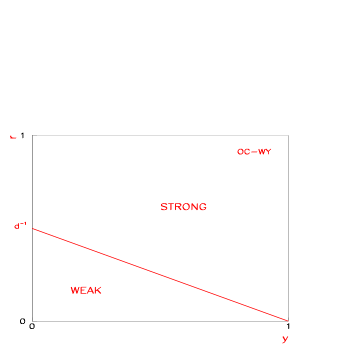
Figure 1: Sketch of the Yukawa phase diagram for a OC Wilson-Yukawa model.

Two phases were found. In the weak phase $y+d\;r\leq 1$, the fermion masses behave as in perturbation theory in the continuum, i.e.

$$m\sim\langle\omega\rangle,$$ (21)

both for doublers and light modes. If the $\omega$ fields have only short-ranged correlations , $\langle\omega\rangle=0$, and the light-fermion spectrum is composed of massless fermions, but there is doubling. However, also a strong phase was found for $y+d\;r\geq 1$ where fermions get masses proportional to a chirally invariant condensate:

$$m\sim\langle{\mbox{R}e}[\omega(x)\omega^{\dagger}(x+\hat{\mu})\;]\rangle^{-1/2}.$$ (22)

This condensate is non-zero in general, and thus all fermions get masses of the order of the cutoff in this phase, even though chiral symmetry is not broken. Since the couplings to the condensate are different for the light and doubler modes, there is a splitting in the masses of the two sectors, and in particular the light-fermion masses can be tuned to zero (at least some of them) by a tuning of the bare mass $y$ to some critical value, while the doublers, whose masses are proportional to $r$, remain massive. The problem in this phase is that the light-fermion spectrum is vector-like. The reason for this is that, owing to the strong Wilson-Yukawa couplings, mirror states can be formed, which are composites of the original fermions and the scalars. In particular, OC studies showed strong evidence that the composite Dirac field

$$\Psi^{(n)}\equiv\omega\Psi_{L}+\Psi_{R}$$ (23)

actually formed. Since it transforms vectorially under the global group, a Dirac mass is not incompatible with the exact chiral symmetry (20). This field is called neutral, because it is neutral under the $U(1)_{L}$, which is the group that is gauged when $g>0$. There is also a charged Dirac fermion,

$$\Psi^{(c)}\equiv\Psi_{L}+\omega^{\dagger}\Psi_{R},$$ (24)

which is neutral under the $U(1)_{R}$ and transforms vectorially under the $U(1)_{L}$. OC studies showed evidence [15] that the charged composite fermion is not formed and the state that propagates in this channel is a two-particle state, $\omega^{\dagger}\Psi^{(n)}$. In any case, the light-fermion spectrum is not the expected one. Either there are no light charged fermions or they couple vectorially to the gauge field. These models do not give rise to a chiral gauge theory.

Again, the TC formulation changes this picture considerably. The main difference is that the high Fourier modes of the $\omega$ field are suppressed (15) which implies that the coupling of the scalars to the light-fermion mode $p\rightarrow 0$ is weak for $r=O(1)$ and $y\ll 1$.

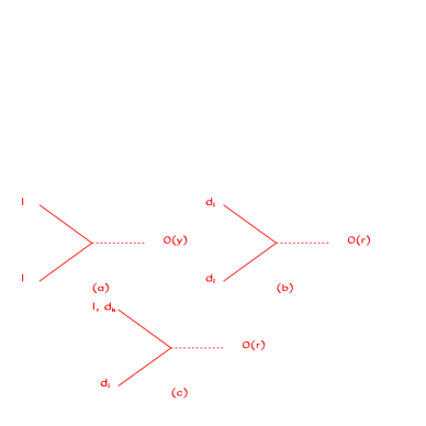
Figure 2: Strength of the couplings of the light $l$ and doubler modes $d_{i}$ to the scalar field $\omega$ (dashed line) in the OC case.

Then, the light lattice modes of the original fermion fields, $\Psi_{L}$ and $\Psi_{R}$, are expected to remain massless according to (21); in other words the poles at $p\rightarrow 0$ of the corresponding propagators are not lifted by the interaction with the $\omega$ fields, because this interaction is weak. The reason why this reasoning fails in OC formulations is that the light-fermion modes have strong couplings to the scalar and other doubler modes ((c) in Fig. 2). These couplings cannot be treated perturbatively. In the TC formulation, these mixed couplings are small, because they involve high Fourier modes of the scalar field, which are strongly suppressed thanks to the cutoff separation. On the other hand, the fermion doubler poles are still strongly coupled to $\omega$ (the diagonal couplings, (b) in Fig. 2, are the same for OC and TC) for $r=O(1)$ and we expect them to get masses according to (22). Thus the fermion propagators will not have doubler poles.

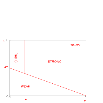
Figure 3: Sketch of the expected phase diagram for a TC Wilson-Yukawa model. The line separating the strong and chiral phases might not be vertical.

In summary, the expected Yukawa phase diagram for the TC formulation is depicted in Fig. 3. A truly chiral phase is expected for $r\geq 1$ and $y\ll 1$, in which the only massless modes are those corresponding to the poles at $p=0$ of the fields $\Psi_{L}$ and $\Psi_{R}$, in (19). This is the correct fermion spectrum to define a chiral gauge theory.

4 A Two-Dimensional Model

As we argued in the previous section, the first non-trivial test of any lattice regularization of chiral gauge theories is to obtain, at zero gauge coupling, undoubled chiral fermions at finite lattice spacing. Extensive numerical studies in OC formulations [12] have shown that this is highly non-trivial, already in the quenched approximation. In this section, I will review our numerical results [13] on the fermion spectrum in a $U(1)$ chiral model in 2D with the TC formulation, which support the expectation that a chiral undoubled spectrum is present, as shown in Fig. 3.

At zero coupling, ${\not\!\!D}$ is trivial, since it reduces to the free operator. However, as we have seen, ${\hat{D}}$ is not, because it is coupled to the pure gauge transformations, which are not suppressed at $g=0$. $\hat{D}$ is obtained from the action (2). The expression of $u_{\mu}$ as a function of $U_{\mu}$ can be found in ref. [13]. Alternatively, in the Wilson-Yukawa picture, the $g=0$ limit corresponds to setting $U_{\mu}=1\rightarrow u_{\mu}=1$ in (19) and what remains is a model of fermions coupled to the scalars $\omega(x)$ with a global $U(1)_{L}\times U(1)_{R}$ symmetry. (In the case $b=f$, this model is identical to the Wilson-Yukawa model considered in [14] for $\kappa=0$). In this limit, the $\omega$ fields depend only on the $\Omega$. The reader is referred to [13] for the explicit formulae.

There are two non-trivial checks to be performed in this global limit. One concerns the phase of the determinant of ${\hat{D}}[u^{\omega}]$, which should vanish in this limit, up to corrections of $O(f/b)^{2}$ according to (8). The second concerns the fermion propagator $G[u^{\omega}[U]]$, which should describe two free massless undoubled fermions (for each charged fermion in (19)), with the same quantum numbers under the $U(1)_{L}\times U(1)_{R}$ global symmetry as $\Psi_{L}$ and $\Psi_{R}$ in (19).

Concerning the phase of the determinant, a numerical test of the expected power counting (8) is shown in Fig. 4. The three histograms correspond to the phase of the fermion determinant ($Phase(\det_{f}({\hat{D}}))$ in the background of $\omega$ configurations generated by interpolation of $\Omega$ configurations generated with the measure ${\cal D}\Omega$ in (14) (i.e. randomly), and for three values of the cutoff ratio $f/b=1,1/4,1/8$ and a $b$-lattice size of $L/b=4$. We refer to the TC lattice sizes with the notation $(L/b)_{(b/f)}$. The charged-fermion content is anomaly-free: four left-handed fields with gauge charge $q_{L}=1$ and one right-handed one with charge $q_{R}=2$. Clearly the change in the phase gets smaller with the ratio $f/b$, as expected, and this implies that the $\omega$ fields are weakly coupled in $\Gamma[u^{\omega}[U]]$. As we have argued, this is important to ensure that they will decouple from the light spectrum so that an effective gauge-invariant theory with no extra scalar degrees of freedom will be obtained at large distances.

Figure 4: $Phase(\det_{f}({\hat{D}}))/\pi$ in the background of $\omega$ configurations obtained from the measure ${\cal D}\Omega$ in lattice sizes $4_{1}$, $4_{4}$ and $4_{8}$.

To study the fermion spectrum described by the propagator $G[u^{\omega}[U]]$, we are going to consider the quenched approximation. In this case, we can simplify the charged-fermion content to just one left-handed fermion with charge 1, since the anomaly is not present in this limit. The reason why this approximation is sensible is because, as we have just seen, in the TC construction, fermion-loop corrections to the $\omega$ effective Lagrangian are suppressed by powers of $f/b$, if gauge anomalies cancel. Thus, for small enough $f/b$, the scalar measure is going to be dominated by ${\cal D}\Omega$ in the limit of zero gauge coupling.

In the quenched approximation, the correlation length of the $\omega$ fields only depends on the interpolation. In Fig. 5, we show the scalar propagator in time:

$$S_{\omega}(t)=\langle\omega^{\dagger}(x_{1},x_{2})\;\omega(x_{1},y_{2})\rangle\;\;\;t=|y_{2}-x_{2}|,$$ (25)

where $x_{1}$ and $y_{1}$ are chosen randomly for every configuration. Even though the interpolation is not strictly local, the decay at large times of $S_{\omega}$ can be fitted to an exponential. The correlation length obtained is of $O(1)$ in $b$-units. This indicates that the scalar field decouples at large distances with respect to $b$ as a massive particle with a mass of the order of the boson cutoff. Provided $f/b$ is small enough, this will not change when the quenched approximation is relaxed.

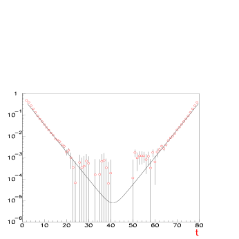
Figure 5: Scalar propagator (25) in a $20_{4}$ lattice.

4.1 Fermion Spectrum

We have computed the fermion propagators:

$$S_{ij}^{a}(t)=\langle\sum_{x_{1},y_{1}}\;\;\Psi_{i}^{(a)}(x)\bar{\Psi}_{j}^{(a)}(y)\;\;e^{ip_{1}(y_{1}-x_{1})}\;\;\rangle_{\Omega},\;\;\;\;\;t=|y_{2}-x_{2}|,$$ (26)

where $t=1,...,L$, the index $a$ refers to the neutral (n) (23), charged (c) (24) or physical ($\Psi_{L}+\Psi_{R}$) (p) fermion for $p_{1}=0$, and the corresponding spatial doublers (nd), (cd) and (pd) for $p_{1}=\pi$. The indices $i,j=R,L$ to the different chiralities. The physical propagator corresponds to ${\hat{D}}^{-1}$, while the neutral and charged ones are easily obtained from it. For every inversion, the time slice at the origin $x_{2}$ is chosen randomly. The number of sampled scalar configurations is typically of $O(2$–$5\ 10^{2})$. The matrix inversions have been performed with the conjugate-gradient method for several values of $y$ and fixed $r=1$. According to the expected Yukawa phase diagram in Fig. 3, we should find a different spectrum for large and small $y$.

At large $y\gg f/b$, we find that all the fermions are massive, as was also found in OC studies. Of course this phase has no physical interest, since all the particles, scalars and fermions, have masses of the order of the cutoff. However, it is useful to understand how fermion masses are generated even if chiral symmetry is not broken. We find that the neutral propagator in momentum space is well reproduced by the hopping parameter expansion [12] (an expansion in $1/(y+2r)$). To first order in this approximation, the neutral field is a free Wilson fermion with

$$y_{eff}=\frac{y}{z},\;\;\;\;\;\;r_{eff}=\frac{r}{z},$$

$$Z_{L}=z^{-1},\;\;\;Z_{R}=1,$$ (27)

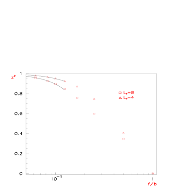
Figure 6: $z^{2}$ condensate for two lattice sizes $L/b=8,4$ as a function of the ratio $f/b$. The lines are quadratic fits.

where $Z_{L,R}$ are the wave-function renormalization constants of the $\Psi^{(n)}_{L,R}$ fields, respectively, and $z$ is the strong condensate

$$z^{2}\equiv\;\langle{\mbox{R}e}(\omega(x)\omega^{\dagger}(x+\hat{\mu}))\rangle_{\Omega},$$ (28)

justifying formula (22). In Fig. 6, we show the value of this condensate for two $b$-lattice sizes as a function of $f/b$. It is easy to show that

$$\lim_{f/b\rightarrow 0}\;\;z^{2}=\;\;1.$$ (29)

In Fig. 7, we show two of the components of the neutral propagator $S^{(n)}_{LR}$ and $S^{(n)}_{RL}$ in momentum space, together with the fits to the free Wilson formulae for $y=1.5$ in an $8_{8}$ lattice. The fitted values of $y_{eff}$ and $r_{eff}$ are in good agreement with the hopping result (27).

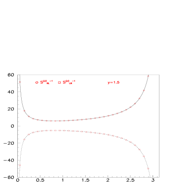
Figure 7: $(S^{(n)}_{RL,LR})^{-1}$ at $y=1.5$ and a lattice size of $8_{8}$. The lines correspond to the fits to the free Wilson fermion formulae. The parameters of the fits for $S^{(n)}_{LR}$ are $Z_{L}^{2}=1.175(8)$, $y_{eff}=1.628(5)$ and $r_{eff}=1.083(4)$, while the hopping result is $Z_{L}^{2}=1.177$, $y_{eff}=1.627$ and $r_{eff}=1.085$.

The neutral spatial doubler also shows good agreement with the hopping result.

The charged propagator (24) is also massive, as can be seen in Fig. 8. However, the hopping expansion is not a good approximation in this case. Our data are also consistent with the charged channel being dominated by the two-particle state $\omega^{\dagger}\Psi^{(n)}$, as was found in OC studies [15].

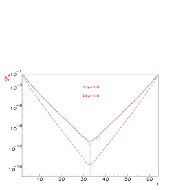
Figure 8: $S^{(c)}_{RL}$ propagators in time for $y=1,1.5$. The lines following the data points are the result of the two-exponential fits.

Finally, for the physical field, we have $S^{(p)}_{RL}=S^{(n)}_{RL}$ and $S^{(p)}_{LR}=S^{(c)}_{LR}$. The chirally breaking components $S^{(p)}_{LL,RR}$ are compatible with zero, as they should be if chiral symmetry is exact.

As we decrease $y\leq 1$, the different chiral components of both the light neutral and charged propagators start to differ. Two components get lighter than the others: $S^{(n)}_{RL}=S^{(p)}_{RL}$ and $S^{(c)}_{LR}=S^{(p)}_{LR}$ (i.e. the expected physical fields). There is a critical value of $y_{c}$ below which the two lighter components $S^{(n)}_{RL}$ and $S^{(c)}_{LR}$ get massless at finite lattice spacing. This is the onset of the announced chiral phase.

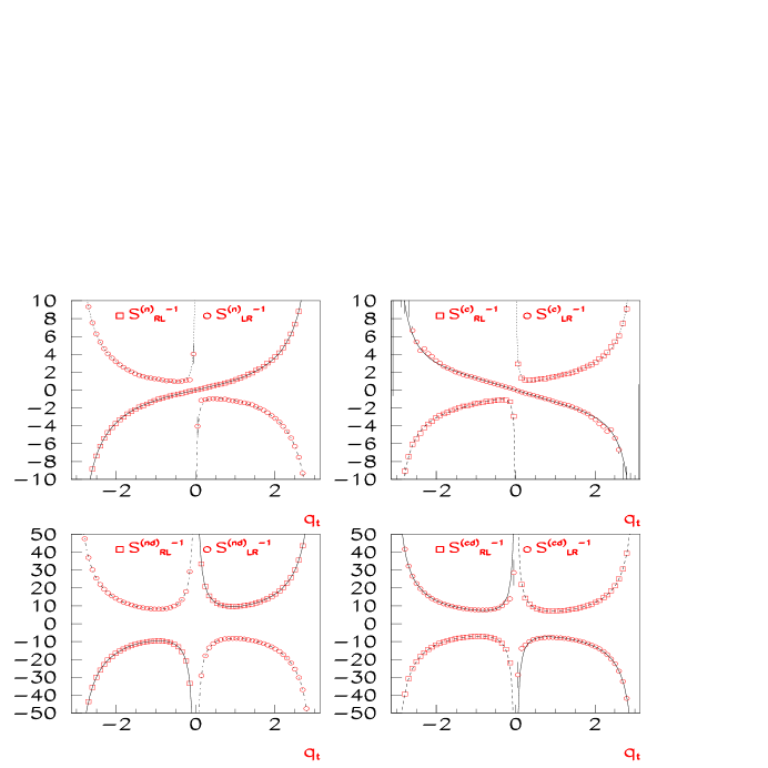
Figure 9: Inverse propagators $(S^{(n),(nd)})^{-1}$ and $(S^{(c),(cd)})^{-1}$ in momentum space in an $8_{8}$ lattice for $y=0.05$.

In Fig. 8, we show the $RL$ and $LR$ components of the neutral (n), charged (c) and the corresponding spatial doublers (nd) and (cd) inverse propagators in momentum space for $y<y_{c}$. Clearly there are only two components with poles at $q=0$: $S^{(n)}_{RL}=S^{(p)}_{RL}$ and $S^{(c)}_{LR}=S^{(p)}_{LR}$, that is the original fields in the Lagrangian (14). These propagators show no other poles in momentum space, as expected from undoubled fermions. None of the other components of the neutral and charged propagators, nor any of the doublers, have any pole in the whole Brillouin zone. So the only massless modes are those expected. The doubler propagators $\Psi^{(n)}$ and $\Psi^{(c)}$ behave as massive Dirac fields, supporting the expectation that the doubler modes remain in the strong phase. The dependence on $y$ for $y<y_{c}$ is negligible. Also the volume effects for fixed $f/b$ ratio are very small [13]. On the other hand, the dependence on the ratio $f/b$ seems very important. We have found that, as this ratio increases, the splitting between the doubler and light sector decreases dramatically. This indicates the importance of the cutoff separation to ensure the doubler-light splitting.

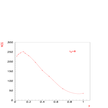
Figure 10: Number of conjugate-gradient iterations in the inversion of the neutral propagator as a function of $y$ in an $8_{8}$ lattice.

It is not clear what determines the value of $y_{c}$. There is one obvious candidate, which is the boson cutoff, i.e. $f/b$ in $f$-lattice units. We have monitored the number of conjugate gradient iterations (NCG) required in the fermion matrix inversion, which is related to the minimum eigenvalue of the matrix. As $y$ decreases, the mass of the fermions decreases, and so does the lowest eigenvalue of the fermion matrix, so that NCG grows. However, when we enter the chiral phase, the lowest eigenvalue is the IR cutoff since there are massless fermions, so the NCG should not grow further. In Fig. 9 we show the NCG as a function of $y$. We find a maximum where we expect $y_{c}$ to be, according to the behaviour of the propagators. It is located around $f/b$ for this lattice size. The physical picture behind this expectation is nothing but the FNN conjecture that at distances larger than $b/f$ in $f$-units, the scalars should decouple. The correlation length of the light fermions in the strong phase is $\sim y$, so when $y<f/b$ the scalars decouple from the light fermions and a chiral phase appears.

More statistics will be needed to understand the properties of the transition at $y_{c}$. In any case, the numerical evidence in this simple model supports the expectation that the chiral phase in Fig. 3 exists, which has the correct light fermionic degrees of freedom to obtain a chiral gauge theory. Similar conclusions are expected in 4D models.

References

References

- [1] A. Borrelli et al., Nucl. Phys. B333(1990) 335-356. L. Maiani, G.C.Rossi and M. Testa, Phys. Lett. B292(1992) 397. See also M. Testa in these procceedings.
- [2] P. Hernández and R. Sundrum, Nucl. Phys. B455(1995) 287.
- [3] P. Hernández and R. Sundrum, Nucl. Phys. B472(1996) 334.
- [4] For other interpolations see M. Lüscher, Commun. Math. 85(1982)39.
- [5] D. Foester, H.B. Nielsen and M. Ninomiya, Phys. Lett. B94(1980) 135.
- [6] S.A. Frolov and A.A. Slavnov, Nucl. Phys. B411(1994) 647; A.A.Slavnov, Phys. Lett. B319(1993) 231.
- [7] G. t’ Hooft, Phys. Lett. B349(1995) 491.
- [8] R. Flume and D. Wyler, Phys. Lett. B108(1982) 317. M. Göckeler, A. Kronfeld, G. Schierholz and U.J. Wiese, Nucl. Phys. B404(1993) 839-582. M. Gockeler, G. Schierholz, Nucl. Phys. B(Proc. Supp.) 29B,C (1992).
- [9] L. Alvarez-Gaumé and S. Della Pietra, in Recent developments in quantum field theory, eds. J. Ambjorn, B.J. Durhuus and J.L. Petersen (North Holland, Amsterdam, 1985). G.T. Bodwin and E.V.Kovacs, Nucl. Phys. B (Proc. Suppl.) 30(1993) 617.
- [10] M. Göckeler, A. Kronfeld, G. Schierholz and U.J. Wiese, Nucl. Phys. B404(1993) 839-582. Y. Shamir, Review Talk at Lattice 95, Nucl. Phys. B(Proc. Supp.) 47 (1996).
- [11] See M. Testa in these proccedings.
- [12] J. Smit, Nucl. Phys. B (Proc. Suppl.) 9 (1989) 579. S. Aoki, I.H.Lee and S-S. Xue, Phys. Lett. B229(1989) 403. S. Aoki, I.H. Lee, J. Shigemitsu and R.E. Shrock, Phys. Lett. B229(1989) 403. S.Aoki, I.H. Lee and R.E. Shrock, Nucl. Phys. B355(1991) 383. W.Bock et al., Phys. Lett. B232(1989) 486. I.M. Barbour et al., Nucl. Phys. B368(1992) 390. M.F.L. Golterman, D.N.Petcher and J.Smit, Nucl. Phys. B370(1992) 370. W. Bock et al., Nucl. Phys. B371(1992) 683. W. Bock, A.K. De, and J. Smit, Nucl. Phys. B388(1992) 243.
- [13] P. Hernández and Ph. Boucaud, hep-lat/9706021.
- [14] W. Bock, A.K. De, E. Focht and J. Smit, Nucl. Phys. B333(1990) 335-356.
- [15] M.F.L. Golterman, D.N. Petcher and E. Rivas, Nucl. Phys. B377(1992) 405.