Abstract

We explore the effect of higher order operators in the non-relativistic formulation of QCD (NRQCD). We calculated masses in the $b\bar{b}$-spectrum using quenched gauge configurations at $\beta=6.0$ and two different NRQCD actions which have been corrected to order $mv^{4}$ and $mv^{6}$. The two-point functions are calculated in a gauge invariant fashion. We find the general structure of the spectrum to be the same in the two cases. Using the $1\bar{P}-1{}^{3}S_{1}$ splitting we determine the inverse lattice spacings to be 2.44(4) GeV and 2.44(5) GeV for the $mv^{4}$ and $mv^{6}$ actions, respectively. We do observe shifts in the spin splittings. The hyperfine splitting is reduced by approximately 4 MeV, while the fine splitting is down by up to 10 MeV, albeit with large statistical errors.

1 Introduction

Heavy quark systems have long been studied and much experimental data has been accumulated which will eventually lead to tight constraints on the parameters of the Standard Model. To this end it is important to have accurate non-perturbative predictions from QCD which can be compared with experiment. One such method is Lattice QCD and it is necessary to understand how heavy quark systems can be treated in this framework.

A nonrelativistic approximation to QCD, NRQCD, was proposed [1] to go beyond the static approximation in lattice calculations. NRQCD has been remarkably successful in reproducing the spectrum of heavy quark systems [2, 3, 4, 5] owing to the fact that the quarks within such hadrons move with velocities $v$ such that $v^{2}\ll c^{2}$. Furthermore, NRQCD has the virtue of retaining, at least approximatively, the quark dynamics and can be considered an effective theory. Computationally, such an approach is much faster to solve than the inversion problem in fully relativistic QCD. A systematic improvement program has been developed to match lattice NRQCD to continuum QCD [6, 7]. As an effective field theory the predictive power of NRQCD relies on the control of higher dimensional operators.

In this paper we calculate the $b\bar{b}$ spectrum comparing two different NRQCD-actions with accuracies $O(mv^{4})$ and $O(mv^{6})$. In section 2 we give the details of our evolution equation and the gauge invariant operators used. In section 3 we state the results and convert them into dimensionful units. In the concluding section we compare our results with other work in this area and experimental data.

2 NRQCD and Operators

In NRQCD the inversion problem of the fermion matrix is an initial value problem. We use the evolution equation along the Euclidean time-direction defined by:

$$G({\bf x},t+1;y) = \left(1-\frac{aH_{0}}{2n}\right)^{n}U_{t}^{{\dagger}}(x)\left(1-\frac{aH_{0}}{2n}\right)^{n}\left(1-a\delta H\right)G({\bf x},t;y)~{}~{},~{}~{}~{}~{}~{}t\geq t_{y}+1~{}~{},$$

$$G({\bf x},t_{y}+1;y) = \left(1-\frac{aH_{0}}{2n}\right)^{n}U_{t}^{{\dagger}}(x)\left(1-\frac{aH_{0}}{2n}\right)^{n}S({\bf x;y})~{}~{}.$$ (1)

where

$$H_{0} = -\frac{\Delta^{2}}{2m_{b}}~{}~{},$$

$$\delta H = -c_{0}\frac{\Delta^{4}}{8m_{b}^{3}}-c_{1}\frac{1}{2m_{b}}\sigma\cdot g{\bf B}+c_{2}\frac{i}{8m_{b}^{2}}(\Delta\cdot g{\bf E}-g{\bf E}\cdot\Delta)-c_{3}\frac{1}{8m_{b}^{2}}\sigma\cdot(\tilde{\Delta}\times g{\bf E}-g{\bf E}\times\tilde{\Delta})$$ (2)

$$-c_{4}\frac{1}{8m_{b}^{3}}\{\Delta^{2},\sigma\cdot g{\bf B}\}-c_{5}\frac{1}{64m_{b}^{3}}\{\Delta^{2},\sigma\cdot(\Delta\times g{\bf E}-g{\bf E}\times\Delta)\}-c_{6}\frac{i}{8m_{b}^{3}}\sigma\cdot g{\bf E}\times g{\bf E}$$

$$-c_{7}\frac{a\Delta^{4}}{16nm_{b}^{2}}+c_{8}\frac{a^{2}\Delta^{(4)}}{24m_{b}}~{}~{}.$$

Here $S({\bf x,y})$ is the source at the first timeslice ($t=t_{y}$). We have $S({\bf x,y})=\delta^{(3)}({\bf x,y})$ for a single quark source at the origin, $y$, but we also propagate extended objects with the same evolution equation. The operator $H_{0}$ is the leading kinetic term and $\delta H$ contains the relativistic corrections and spin corrections. The last two terms in $\delta H$ are present to correct for lattice spacing errors in temporal and spatial derivatives. For the derivatives we give the following definitions which are consistent with those of [5, 6]:

$$a\Delta_{i}G(x,y) = U_{i}(x)G(x+\hat{\i},y)-U_{-i}(x)G(x-\hat{\i},y)=\frac{1}{2}\left(e^{a\partial_{i}}-e^{-a\partial_{i}}\right)G(x,y)~{}~{},$$

$$\tilde{\Delta}_{i} = \Delta_{i}-\frac{a^{2}}{6}\Delta_{i}^{+}\Delta_{i}^{\pm}\Delta_{i}^{-}=\partial_{i}+O(a^{4})~{}~{},$$

$$a^{2}\Delta^{2}G(x,y) = \left(\sum_{i=1}^{3}U_{i}(x)G(x+\hat{\i},y)+U_{-i}(x)G(x-\hat{\i},y)\right)-6~{}G(x,y)~{}~{},$$

$$\Delta^{4}G(x,y) = \Delta^{2}(\Delta^{2}G(x,y))~{}~{},$$

$$a^{2}\Delta^{(4)}G(x,y) = \left(\sum_{i=\pm 1}^{\pm 3}U_{i}(x)U_{i}(x+\hat{\i})G(x+2\hat{\i},y)-4U_{i}(x)G(x+\hat{\i},y)+\frac{c}{2}~{}G(x,y)\right)~{}~{},$$

$$c = (4+\frac{2}{u_{0}^{2}})~{}~{}.$$ (3)

For our calculation with accuracy $O(mv^{4})$ we set $c_{4},c_{5}$ and $c_{6}$ to zero and replace $\tilde{\Delta}$ by $\Delta$. In this case we calculate the fields $\bf E$ and $\bf B$ from the clover field $F_{\mu\nu}$ in the standard fashion [6]. To determine the spin splittings with accuracy $O(mv^{6})$ we retain the above coefficients and the improved operator $\tilde{\Delta}$. Correspondingly, we replace standard discretized gauge field term $F_{\mu\nu}$ by

$$\tilde{F}_{\mu\nu}=\frac{5}{3}F_{\mu\nu}-\frac{1}{6}\left(U_{\mu}(x)F_{\mu\nu}(x+\mu)U_{\mu}^{{\dagger}}(x)+U_{-\mu}(x)F_{\mu\nu}(x-\mu)U_{-\mu}^{{\dagger}}(x)-(\mu\leftrightarrow\nu)\right)~{}~{},$$ (4)

when this accuracy is needed for ${\bf E}$ and ${\bf B}$ in Equation 2.

All the gauge links are tadpole improved with $u_{0}=\langle 0|\frac{1}{3}TrU_{\mu\nu}|0\rangle^{1/4}$ as suggested in [8]. It has been demonstrated that tadpole improvement is crucial to reproduce the spin splittings accurately, which are otherwise underestimated. We assume that radiative corrections are sufficiently accounted for by tadpole improvement and we therefore set all the renormalisation coefficients, $c_{i}$, to 1.

To extract masses we calculate two-point functions of operators with the appropriate quantum numbers. In a non-relativistic setting gauge-invariant meson operators can be constructed from the two-spinors $\chi^{{\dagger}}(x)$ and $\Psi(y)$ (which represent the antiquark field and quark field) and a Wilson line, $W(x,y)$. Such operators have the following behaviour under rotation, parity and charge conjugation

$$\chi^{{\dagger}}(x)W(x,y)\Psi(y) \stackrel{{\scriptstyle\cal R}}{{\longrightarrow}} \chi^{{\dagger}}(Rx)W^{\cal R}(Rx,Ry)\Psi(Ry)~{}~{},$$

$$\chi^{{\dagger}}(x)W(x,y)\Psi(y) \stackrel{{\scriptstyle\cal P}}{{\longrightarrow}} -\chi^{{\dagger}}(x_{p})W^{\cal P}(x_{p},y_{p})\Psi(y_{p})~{}~{},$$

$$\chi^{{\dagger}}(x)W(x,y)\Psi(y) \stackrel{{\scriptstyle\cal C}}{{\longrightarrow}} -\Psi^{T}(x)W^{\cal C}(x,y)\chi^{\ast}(y)~{}~{}.$$ (5)

The construction of spatially extended operators on the lattice has been reported elsewhere [9]. Here we adopt the following notation:

$$L_{i}^{n}(x) \equiv U_{i}(x)U_{i}(x+i)\ldots U_{i}(x+(n-1)i)=L_{-i}^{n{\dagger}}(x+in)~{}~{},$$

$$\Delta_{i}^{n}\Psi(x) \equiv L_{i}^{n}(x)\Psi(x+ni)-L_{-i}^{n}(x)\Psi(x-ni)~{}~{}.$$ (6)

With the generalised link variables of equation 6 and the transformation properties of equation 5 we can construct operators with definite $J^{PC}$, where $J$ labels the irreducible representations of the octahedral group ($J=A_{1},A_{2},T_{1},T_{2},E$).

In order to increase the overlap between the meson and the ground states we create on the lattice we use extended versions of the derivative as defined in equation 6. The operators we used are listed in Table 1. The meson correlator is written as a Monte Carlo average over all configurations

$${\rm C}^{nm}(x,y)=\langle{\bf tr}\left[G^{{\dagger}}(x,y)G^{nm}(x,y)\right]\rangle~{}~{},$$ (7)

where ${\bf tr}$ denotes contraction over all internal degrees of freedom and $G^{nm}$ is the smeared propagator defined by

$$G^{nm}(x,y)\equiv\sum_{z_{1},z_{2}}O^{n}(x,z_{1})G(z_{1},z_{2})O^{m{\dagger}}(z_{2},y)~{}~{}.$$ (8)

Here $(n,m)$ stands for the radii at (sink, source) and $O^{n}$ is an operator as defined in Table 1 but with extended symmetric derivative $\Delta^{n}$. For the smeared propagator we solve equation 1 with $S({\bf x,y})=O^{m{\dagger}}({\bf x,y})$ and multiply with $O^{n}$ at the sink. We fix the origin at some (arbitrary) lattice point, $y$, and sum over all spatial ${\bf x}$ so as to project out the zero momentum mode. In addition we sum over all polarisations to increase the statistics.

3 Simulation and Results

We use quenched gauge field configurations at $\beta=6.0$ on a $16^{3}\times 48$ lattice generated with the standard Wilson action at the EPCC in Edinburgh. The propagators were calculated at the HPCF in Cambridge and at the Hitachi Europe Ltd. High Performance Computing Center in Maidenhead. As the operators chosen are gauge invariant, gauge fixing is not necessary. We used the extended operators defined in section 2 with radii 1,2 and 3 in both the source and sink thus giving rise to a $3\times 3$ matrix of correlators for each set of quantum numbers. The calculation were done with a bare quark mass of $am_{b}=1.71$ which is the same as that used in [5]. We used $n=2$ as the stability parameter in Equation 1. The tadpole improvement coefficient appropriate to $\beta=6.0$ is $u_{0}=0.878$ as in [5]. We calculated quark propagators for both actions from 8 points $(i,j,k)$ where $i,j,k$ is $0$ or $7$ on the first timeslice for each of the 499 configurations. It has been noted previously [5] that such an arrangement gives independent and uncorrelated measurements due to the small size of the $b\bar{b}$-system on our lattice. Thus we have a total of 35928 correlators for each meson we considered (${}^{1}S_{0},{}^{3}S_{1},{}^{1}P_{1},{}^{3}P_{0,1,2}$). We also average over all polarisations and all spin components.

We fit the correlators to the multi-exponential form

$$C_{\alpha}^{nm}(t)=\sum_{i=1}^{\rm n_{fit}}a_{\alpha i}^{nm}e^{-M_{i}^{\alpha}t}~{}~{}.$$ (9)

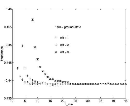
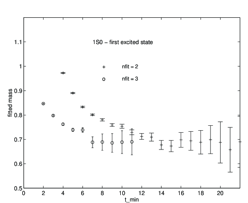
Figure 1: Two examples of correlated fits for the ${}^{1}S_{0}$-state, calculated with the improved action. The different symbols denote different choices for $n_{fit}$ and the $t_{min}$ dependence is shown. This is to demonstrate the consistency of our fit results as we change the fit prescription. We chose $t_{max}=48$ for all fits.

Here $\alpha$ denotes a meson state with certain quantum numbers, $(n,m)$ the different radii at the (sink, source) and $t$ the Euclidean time. We chose ${\rm n_{fit}}$ to be 1,2 or 3 and restrict ourselves to some conveniently chosen subsets of all the data, e.g. a window $[t_{min},t_{max}]$. The basic method for obtaining the parameters $a_{\alpha i}^{nm}$ and $M_{i}^{\alpha}$ (which we generically refer to as $\{b_{l}\}$) is a correlated fit using the whole covariance matrix. The statistical nature of the data causes fluctuations from the central values of the parameters, which are determined from a minimal $\chi^{2}(b)$ fit. We estimate the covariance matrix for the parameters from the inverse of $(\partial^{2}\chi^{2})/(\partial b_{k}\partial b_{l})$. The goodness of the fit is quantified by the $Q$-value, defined in [11]. We require an acceptable fit to have $Q>0.1$ and that the results remain consistent as we alter our fitting prescription slightly (e.g. varying $t_{min}$ or the number of eigenvalues retained when inverting the covariance matrix of the data). To illustrate the method we display a fitted mass plotted against $t_{min}$ in Figure 1. Our dimensionless results for the non-relativistic rest energies are shown in Table 2.

Fitting excitation energies relative to the ground state makes it difficult to extract the splitting and the associated error of the P-state. We rewrite Equation 9 as

$$C_{\alpha}^{nm}(t)=\sum_{i=1}^{n_{\rm fit}}a_{\alpha i}^{nm}e^{-(M_{1}^{1}+\delta{M}_{i}^{\alpha})t}~{}~{},$$ (10)

where we can now fit the amplitudes $a_{\alpha i}^{nm}$, the ground state mass $M_{1}^{1}$ and the splittings, $\delta{M}_{i}^{\alpha}$, with respect to $M_{1}^{1}$. Our results are tabulated in Table 3.

From the $1\bar{P}-1{}^{3}S_{1}$ splitting we estimate the lattice spacing at $\beta=6.0$ to be $a_{\bar{P}-S}^{-1}=2.44(4)$ GeV for the improved action and $a_{\bar{P}-S}^{-1}=2.44(5)$ GeV for the unimproved action. The kinetic masses were determined using 80 configurations for both actions. We show an example of the dispersion relation in Figure 2 and the results are shown in Table 4.

4 Conclusions

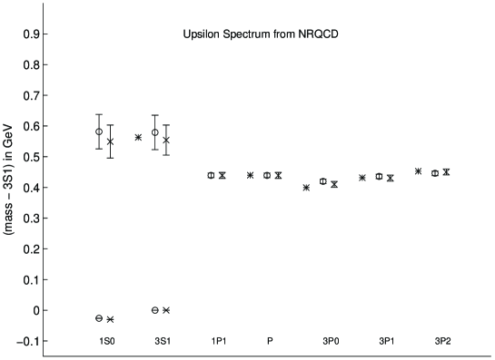
Figure 3: Upsilon spectrum. We compare our results for two actions with different accuracies. Crosses are the results from an action which is accurate to $O(mv^{4})$. Circles denote an improved calculation where spin-corrections, $c_{4},c_{5}$ and $c_{6}$, have been taken into account up to order $O(mv^{6})$. Bursts denote the experimental value where available. The splittings, relative to the ${}^{3}S_{1}$, are shown. The scale has been calculated from the $1\bar{P}-1{}^{3}S_{1}$ splitting.

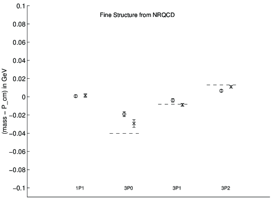
Figure 4: Upsilon fine structure. The splittings, relative to the $\bar{P}$, are shown. Experimental values are shown as dashed lines. Crosses denote accuracy up to $O(mv^{4})$, circles up to $O(mv^{6})$. The scale has been calculated from the $1\bar{P}-{}^{3}S_{1}$ splitting.

Despite the success of NRQCD, a source of concern has been the effect of higher dimensional operators in ${\cal L}_{NRQCD}$. To test this issue, we calculated the $\Upsilon$ spectrum in a gauge invariant fashion to accuracy $O(mv^{4})$. We then retained the spin corrections in Equation 1 up to $O(mv^{6})$ and compared the results with each other. We also checked higher order contributions to the derivative in the term proportional to $c_{3}$ and found their effect negligible. Our main results are summarised in Figures 3 and 4. In Table 3 we compare the results for the two different evolution equations with each other and convert the dimensionless numbers into physical units. We set the scale using the $1\bar{P}-1{}^{3}S_{1}$ splitting and find $a^{-1}_{\bar{P}-S}=2.44(4)$ GeV and $2.44(5)$ GeV, respectively. Our results for a lower order evolution equation match those from an earlier calculation [5, 13, 14] where the configurations were fixed in the Coulomb gauge.

These comparisons demonstrate the consistency of NRQCD. The gross structure of the $\Upsilon$-spectrum calculated is unchanged when we added the spin correction terms. For example, the ratio $R_{SP}=(2{}^{3}S_{1}-1{}^{3}S_{1})/(1\bar{P}-1{}^{3}S_{1})=1.3(1)$ agrees for both actions and with the experimental value, 1.28, within statistical errors.

The bare mass parameter, $am_{b}$, was chosen to be 1.71 to match a choice in [5]. With our lattice spacing this corresponds to $m_{b}=4.17(7)$ GeV and gives a kinetic mass of $9.4(3)$ GeV (for the $mv^{6}$ action) and $9.7(3)$ GeV (for the $mv^{4}$ action) which should be compared to the experimental value of $9.46$ GeV. The differences in the kinetic mass due to the extra terms is of the order of 1-2 standard deviations. We note also that the $\chi^{2}/$dof resulting from the kinetic mass fits for the $mv^{6}$ action is much smaller than that for the $mv^{4}$ action.

However, differences can be seen for the spin splittings. The introduction of the extra terms reduces the hyperfine splitting, ${}^{3}S_{1}-{}^{1}S_{0}$, by approximately 4 MeV. This size of a shift is what one would expect from power counting arguments.

We also observe a reduction in the fine structure. For example, by adding the spin corrections the ${}^{3}P_{2}-{}^{3}P_{1}$ splitting is reduced from 19(3) MeV to 11(3) MeV, compared with the experimental value of 21 GeV. Such a behaviour has also been reported for the spectrum calculations of charmonium on much coarser lattices [12]. Here we find a similar tendency and further analysis will be needed to decide whether this feature persists in unquenched calculations. We note that the ratio $R_{fs}=(1{}^{3}P_{2}-1{}^{3}P_{1})/(1{}^{3}P_{1}-1{}^{3}P_{0})=0.56(19)$ from our improved calculation is in better agreement with the experimental value (0.66). For the less accurate action we find 1.11(26) for this ratio.

There will be additional uncertainties due to radiative corrections to the coefficients $c_{i}$ in ${\cal L}_{NRQCD}$. Discretisation errors in the gluonic action will also effect our results and of course there will be corrections due to the introduction of sea quarks. Future studies into the accuracy of NRQCD will have to address these systematic errors.

Acknowledgements

We would like to thank other members of the UKQCD collaboration in particular C.T.H. Davies and S. Collins for useful discussions. T.M. wishes to thank J. Sloan for discussing details of the evolution equation. This research is supported by a grant from EPSRC (Ref. No. 94007885) and in parts by a grant from the European Union (ERBCHB6-CT94-0523). Our calculations are performed on the Hitachi (S3600 and SR2001) located at Hitachi Europe’s Maidenhead (United Kingdom) headquarters, the University of Cambridge High Performance Computing Facility and the CRAY-T3D at the Edinburgh Parallel Computing Centre at Edinburgh University.

Meson	$L\to O_{h}$	$S\to O_{h}$	$(L\otimes S)$	Operator
${}^{1}S^{-+}$	$0\to A_{1}$	$0\to A_{1}$	$A_{1}^{-+}$	$c+\Delta^{2}$
${}^{3}S^{--}$	$0\to A_{1}$	$1\to T_{1}$	$T_{1}^{--}$	$(c+\Delta^{2})\sigma_{i}$
${}^{1}P^{+-}$	$1\to T_{1}$	$0\to A_{1}$	$T_{1}^{+-}$	$\Delta_{i}$
${}^{3}P^{++}$	$1\to T_{1}$	$1\to T_{1}$	$A_{1}^{++}$	$\sigma_{i}\cdot\Delta_{i}$
			$T_{1}^{++}$	$\epsilon_{ijk}\sigma_{j}\Delta_{k}$
			$T_{2}^{++}$	$\sigma_{k}\Delta_{j}+\sigma_{j}\Delta_{k}$
			$E^{++}$	$\sigma_{j}\Delta_{j}-\sigma_{k}\Delta_{k}$

Table 1: transformation behaviour of $b\bar{b}$-states in their non-relativistic notation

State	$aM_{mv^{6}}$	$aM_{mv^{4}}$	$aM_{mv^{4}}-aM_{mv^{6}}$
$1^{1}S_{0}$	0.4391(3)	0.4416(3)	0.00265(5)
$2^{1}S_{0}$	0.688(23)	0.679(22)	–
$1^{3}S_{1}$	0.4497(4)	0.4539(3)	0.00439(6)
$2^{3}S_{1}$	0.687(23)	0.681(20)	–
$1S$	0.4470(3)	0.4508(3)	0.00396(9)
$2S$	0.69(3)	0.68(2)	–
${}^{1}P_{1}$	0.632(7)	0.635(7)	0.0033(1)
${}^{3}P_{0}$	0.619(7)	0.621(7)	0.0021(2)
${}^{3}P_{1}$	0.628(7)	0.627(8)	0.0029(1)
${}^{3}PT_{2}$	0.635(5)	0.642(6)	0.0053(1)
${}^{3}PE_{2}$	0.632(7)	0.642(6)	0.0055(1)
$\bar{P}$	0.630(3)	0.634(4)	0.0042(1)

Table 2: Here we compare the absolute masses from different evolution equations and calculate their difference from a ratio fit with bootstrap errors.

Splitting	$O(mv^{6})$	$\times~{}~{}a^{-1}$ [GeV]	$O(mv^{4})$	$\times~{}~{}a^{-1}$ [GeV]	Exp. value
		[2.44(4)]		[2.44(5)]
$\bar{P}-1{}^{3}S_{1}$	0.180(3)	0.4398	0.180(4)	0.4398	0.4398 GeV
$1^{3}S_{1}-1{}^{1}S_{0}$	0.01073(5)	0.0262(6)	0.01227(11)	0.0300(7)	–
$2^{3}S_{1}-1{}^{3}S_{1}$	0.24(2)	0.59(5)	0.23(2)	0.56(5)	0.5629 GeV
$1^{1}P_{1}-1{}^{3}S_{1}$	0.180(6)	0.440(18)	0.181(7)	0.442(20)	–
$1^{3}P_{2}-1{}^{3}P_{0}$	0.011(2)	0.027(5)	0.0143(34)	0.035(8)	0.0534 GeV
$1^{3}P_{2}-1{}^{3}P_{1}$	0.0045(14)	0.011(3)	0.0078(11)	0.019(3)	0.0213 GeV
$1^{3}P_{1}-1{}^{3}P_{0}$	0.008(1)	0.019(2)	0.0070(13)	0.017(3)	0.0321 GeV
$1^{3}P_{2}-\bar{P}$	0.00272(55)	0.0066(14)	0.0045(5)	0.011(1)	0.0131 GeV
$\bar{P}-1^{3}P_{1}$	0.0016(8)	0.004(2)	0.0036(6)	0.0088(15)	0.0082 GeV
$\bar{P}-1^{3}P_{0}$	0.0078(11)	0.019(3)	0.0120(17)	0.029(4)	0.0403 GeV
$M_{kin}$	3.84(8)	9.38(25)	3.97(8)	9.70(29)	9.4604 GeV
$R_{SP}$	1.33(11)		1.28(11)		1.2802
$R_{fs}$	0.56(19)		1.11(26)		0.6636

Table 3: Summary of splittings. We show our results for both accuracies and convert them into physical units. The lattice spacing is determined from the $1\bar{P}-1{}^{3}S$ splitting in both cases. $R_{SP}=(2^{3}S_{1}-1{}^{3}S_{1})/(1\bar{P}-1{}^{3}S_{1})$, $R_{fs}=({}^{3}P_{2}-{}^{3}P_{1})/({}^{3}P_{1}-{}^{3}P_{0})$.

State	$aE_{mv^{6}}$	$aE_{mv^{4}}$	$aE_{mv^{4}}-aE_{mv^{6}}$
$1^{1}S_{0}({\bf p}=(1,0,0))$	0.458(1)	0.462(1)	0.00236(7)
$1^{1}S_{0}({\bf p}=(1,1,0))$	0.478(2)	0.481(2)	0.00212(8)
$1^{1}S_{0}({\bf p}=(1,1,1))$	0.496(4)	0.499(3)	0.00191(10)
$1^{1}S_{0}({\bf p}=(2,0,0))$	0.522(4)	0.524(5)	0.0018(3)
$aM_{kin}$	3.77(7)	3.93(7)
$1^{3}S_{1}({\bf p}=(1,0,0))$	0.469(1)	0.474(2)	0.00427(5)
$1^{3}S_{1}({\bf p}=(1,1,0))$	0.489(2)	0.493(2)	0.00416(6)
$1^{3}S_{1}({\bf p}=(1,1,1))$	0.508(2)	0.511(3)	0.00406(7)
$1^{3}S_{1}({\bf p}=(2,0,0))$	0.531(5)	0.535(5)	0.00417(8)
$aM_{kin}$	3.84(8)	3.97(8)

Table 4: The dispersion relation for ${}^{1}S_{0}$ and ${}^{3}S_{1}$. The momentum is given in lattice units of ${\bf p}=\frac{2\pi}{L}(i,j,k)$ where $L=16$. The last column is the difference for both evolution equations as obtained from a ratio fit.

Figure 2: Dispersion relation for ${}^{3}S_{1}$ and two different accuracies. The non-relativistic energy in lattice units is plotted vs. $(\frac{2\pi}{16})^{2}|{\bf n}|^{2}$ where ${\bf n}=(1,0,0),{\bf n}=(1,1,0),{\bf n}=(1,1,1)$. From this we determine its kinetic mass to be $9.7(3)$ GeV ($O(mv^{4})$) and $9.4(3)$ GeV ($O(mv^{6})$) for $am_{b}=1.71$.

References

- [1] B. Thacker and G. P. Lepage, Phys.Rev.D 43 (1991), 196-208
- [2] C.T.H. Davies and B. Thacker: Nucl. Phys. B 405 (1993), 593-622
- [3] S. Catterall, F. Devlin, I.T. Drummond and R.R. Horgan: Phys. Lett. B 300 (1993), 393-399
- [4] S. Catterall, F. Devlin, I.T. Drummond and R.R. Horgan: Phys. Lett. B 321 (1994), 246-253
- [5] C.T.H. Davies et al., Phys.Rev. D 50 (1994), 6963-6077
- [6] G. P. Lepage et al., Phys.Rev. D 46 (1992), 4052-4067
- [7] C. J. Morningstar, Phys. Rev. D48 (1993), 2265-2278
- [8] G. P. Lepage and P.B. Mackenzie: Phys.Rev. D 48 (1993), 2250-2264
- [9] C. Michael, Phys.Rev. D 54 (1996), 6997-7009
- [10] C. Davies et al., Phys.Rev.Lett. 73 (1994), 2654-2657
- [11] W.H. Press et al., “Numerical recipes in Fortran”, (2nd Edition), Cambridge University Press (1992)
- [12] H.D. Trottier: Phys. Rev. D55 (1997) 6844-6851
- [13] C.T.H. Davies, “The spectrum from Lattice NRQCD”, Nucl. Phys. B Proc. Suppl. (in press)
- [14] C.T.H. Davies et al., “Scaling of the -spectrum” (in preparation)