Random Surfaces in Three-Dimensional Simplicial Gravity

H.S.Egawa and N.Tsuda,

^† Department of Physics, Tokai University

Hiratsuka, Kanagawa 259-12, Japan

^‡ Theory Division, Institute of Particle and Nuclear Studies,

KEK, High Energy Accelerator Research Organization

Tsukuba, Ibaraki 305 , Japan

A model of simplicial quantum gravity in three dimensions is investigated numerically based on the technique of the dynamical triangulation (DT). We are concerned with the surfaces appearing on boundaries (i.e., sections) of three-dimensional DT manifold with $S^{3}$ topology. A new scaling behavior of genus distributions of boundary surfaces is found. Furthermore, these surfaces are compared with the random surfaces generated by the two-dimensional DT method which are well known as a correct discretized method of the two-dimensional quantum gravity.

1 Introduction

There has been, over the last few years, remarkable progress in the quantum theory of two-dimensional gravity. Two distinct analytic approaches for quantizing two-dimensional gravity have been established. These are recognized as a discretized[1] and a continuous[2] theory. The discretized approach, implemented by the matrix model technique, exhibits behavior found in the continuous approach, given by Liouville field theory, in a continuum limit. It thus seems to exist strong evidence for the equivalence of the two theories in two dimensions. Numerical methods based on the matrix model, such as that of dynamical triangulation[3] have drawn much attention as alternative approaches to studying non perturbative effects, being also capable of handling those cases where analytical theories cannot yet produce meaningful results. In the dynamical triangulation method, calculations of the partition function are performed by replacing the path integral over the metric to a sum over possible triangulations. Several close studies[4] on the structure of two-dimensional DT surfaces in quantum gravity were made, and it revealed fractal structures of these surfaces.

However, we feel that the relationship between three-dimensional (also four-dimensional) quantum gravity and its discretized model is not yet understood. Over the past few years a considerable number of numerical studies have been made on three-dimensional simplicial quantum gravity[5]. It is generally agreed that the phase transition of three- and four- dimensional simplicial quantum gravity are both first order[6, 7]. The problems are still in controversy. On the other hand, recent numerical results obtained by the dynamical triangulation for three and four dimensions suggest the existences of the scaling behavior near to the critical point[8, 9, 10]. It may be important to note the asymmetric behavior of the order parameter in usual phase diagram. When the coupling strength, $\kappa_{0}$, closes to the critical point from the strong coupling side ($\kappa_{0}<\kappa_{0}^{c}$) which corresponds to the crumple phase, the transition is smooth. On the other hand, when $\kappa_{0}$ closes to the critical point from the weak coupling side ($\kappa_{0}>\kappa_{0}^{c}$) which corresponds to the branched polymer phase, the transition is very rapid. In ref.[8] it is reported that near the critical point belonging to the strong coupling phase the scaling behavior of the mother universe exists and also that no mother universe exists in the weak coupling phase (i.e., branched polymer phase). It seems reasonable to suppose that the model makes sense as long as we close to the critical point from the strong coupling side. We actually observe a double peak histogram structure which is a signal of the first order phase transition for an appropriate large lattice size. Therefore, we carefully chose one of peaks belonging to the strong coupling phase as an ensemble for our simulations[10].

Figure 1: Schematic picture of boundary surfaces ($\Sigma_{1},\Sigma_{2}$ and $\Sigma_{3}$) at distance $d$ and a surface ($\Sigma_{2}^{\prime}$) at distance $d^{\prime}$ in 3D Euclidean space $M$ with $S^{3}$ topology. The mother boundary surface is defined as a surface ($\Sigma_{2}$) with the largest tip volume ($V_{2}$), and the other surfaces are defined as the baby boundary.

This paper is intended as two investigations, firstly, the searching a new scaling property for the boundary surfaces in three-dimensional DT manifolds near the critical point ($\kappa_{0}^{c}$) and, secondary, the relation between these boundary surfaces and two dimensional random surfaces implemented by the matrix model. Below we will consider only three-dimensional DT manifolds with $S^{3}$ topology. We can represent a typical configuration in Fig.1. $M$ denotes a three-dimensional DT manifold with $S^{3}$ topology and $\Sigma_{1}$, $\Sigma_{2}$ and $\Sigma_{3}$ denote the boundaries which are closed and orientable triangulated surfaces at a distance $d$ from an origin ($\times$). The geodesic distance can be recognized as a usual time parameter.

Our model of three-dimensional Euclidean quantum gravity with boundaries may be recognized as a model of a quantum nucleation of the universe in $(2+1)$-dimensional gravity. The nucleation of the universe by a quantum tunneling may be described by going out of the Euclidean signature region to the Lorentzian signature region in a sense of the semiclassical approximation[11]. The nucleation of the universe can be regarded as a topology-changing process in the sense that the universe takes a transition from the initial state with no boundary to the final state with nontrivial topology. We can treat the model in a full quantum way which means that we sum up all of the fluctuations of the three-dimensional metric $g_{\mu\nu}$ and also put no restriction on the boundary surfaces $\Sigma$. Of course, it is possible to introduce the extrinsic curvature on the boundary surface as a physical restriction. The process of a quantum tunneling requests that all the components of the extrinsic curvature vanish (i.e., totally geodesic).

This paper is organized as follows. In Sec.2 we briefly review the model of the three-dimensional dynamical triangulation. In Sec.3 all of our numerical results, especially genus distributions and coordination number distributions for the mother boundary surfaces, are shown. We summarize our results and discuss some future problems in the final section.

2 Model

It is not yet known how to give a constructive definition of three-dimensional quantum gravity. We start with the Euclidean Einstein-Hilbert action,

$$S_{EH}=\int d^{3}x\sqrt{g}\left(\Lambda-\frac{1}{G}R\right),$$ (1)

where $\Lambda$ is the cosmological constant, and $G$ is Newton’s constant of gravity. We use the lattice action of the three-dimensional model with the $S^{3}$ topology, corresponding to the above action, as follows:

$$S(\kappa_{0},\kappa_{3}) = -\kappa_{0}N_{0}+\kappa_{3}N_{3}$$ (2)

$$= -\frac{2\pi}{G}N_{0}+\left(\Lambda^{\prime}-\frac{1}{G}(2\pi-6\mbox{cos}^{-1}(\frac{1}{3}))\right)N_{3},$$

where $N_{i}$ denotes the total number of $i$-simplexes, and $\Lambda^{\prime}=c\Lambda$; $c$ is the unit volume, and $\mbox{cos}^{-1}(\frac{1}{3})$ is the angle between two tetrahedra. The coupling $\kappa_{0}$ is proportional to the inverse of bare Newton’s constant, and the coupling $\kappa_{3}$ corresponds to a lattice cosmological constant.

For the dynamical triangulation model of three-dimensional quantum gravity, we consider a partition function of the form

$$Z(\kappa_{0},\kappa_{3})=\sum_{T(S^{3})}e^{-S(\kappa_{0},\kappa_{3})}.$$ (3)

We sum over all simplicial triangulations, $T(S^{3})$, on a three-dimensional sphere. In practice, we must add a small correction term $\Delta S$ to the lattice action in order to suppress volume fluctuations. The correction term is denoted by

$$\Delta S=\delta(N_{3}-N_{3}^{(\mbox{target})})^{2},$$ (4)

where $N_{3}^{(\mbox{target})}$ is the target value of three-simplexes, and we use $\delta=0.0005$ in all our run. A fine tuning of $\kappa_{0}$ is one of the elaborate works in this model because the critical coupling $\kappa_{0}^{c}$ depends on the size of the system. A $\kappa_{0}^{\mbox{equiv}}$ discussed in ref.[12] is used as the critical value $\kappa_{0}^{c}(N_{3})$ in our simulation. In ref.[12] the parameter $\kappa_{0}$ is tuned to $\kappa_{0}^{\mbox{equiv}}$ using the multicanonical Monte Carlo method such that the heights of double peaks of $N_{0}$ become the same.

3 Measurements

We now define the intrinsic geometry using the concept of a geodesic distance as a minimum length (i.e., minimum step) in the dual lattice between two tetrahedrons in a three-dimensional DT space. Suppose a tree-dimensional ball (3-ball) which is covered within $d$ steps from a reference 3-simplex in the three-dimensional manifold with $S^{3}$ topology. Naively, the 3-ball has a boundary with spherical topology ($S^{2}$). However, because of the branching of the DT space, the boundary is not always simply-connected, and there usually appear many boundaries which consist of closed and orientable two-dimensional surfaces with any topology and nontrivial structures such as links or knots. These two-dimensional boundary surfaces are equivalent to two-dimensional randomly triangulated surfaces with corresponding genuses. In order to discuss the scaling properties of these surfaces, the genus distributions of these surfaces are measured. We should notice that there appear many boundaries with distance $d$ (see Fig.1). The boundaries are divided into two classes: one is a baby boundary and the other is a mother one. The boundaries with small sizes ($\sim{\cal O}(1)$) are called by a baby one. The baby boundaries are originated from the small fluctuations of the three-dimensional Euclidean spaces. We thus think that these surfaces are non-universal objects and then suffer from large finite size effects. In this section, we shall concentrate only on the mother boundary.

Here, we give a precise definition of “baby” and “mother” universes in Fig.1. The mother universe is defined as a boundary surface ($\Sigma_{2}$) with the largest volume ($V_{2}$), and the other surfaces are defined as baby universes.

Figure 2: Measurement of a genus of boundary surface. (a) denotes an example of a irregular configuration. The boundary surfaces in general may have many singular vertices and links. (b) denotes a regular configuration. After we change (a) into (b), we measure the genus of (b).

The problem is whether we can distinguish these two kinds of universes (baby and mother boundary surfaces) in our simulations. The answer is yes. In Fig.3 we plot the tip volumes (correspond to $V_{1}$, $V_{2}$ and $V_{3}$ in Fig.1) distributions near to the critical point ($\kappa_{0}=4.195$ and $\kappa_{3}=2.222$) with appropriate geodesic distances when $N_{3}=32$. This figure tells us that there is one mother boundary whose tip volume is prominent and the others belong to the class of the baby universe. At any rate, we can easily distinguish the mother boundary surface from the others by the measurement of the tip volume.

In ref.[8] it is reported that the surface-area-distributions (SAD) of the mother universe show the scaling behavior near to the critical point but the baby universe does not show a scaling behaviour at all. The important point to note is that in ref.[8] the measurements in the critical region were done in the strong coupling phase. Therefore, we focus on the mother universe near to the critical point taking the limit from the strong coupling phase following subsections $3.1$ and $3.3$. On the other hand, it is known that in the weak coupling limit the three-dimensional DT manifold becomes a branched polymer, and its boundary surfaces show no scaling property[8]. Therefore, we cannot consider the genus distributions of boundary surfaces in the weak coupling phase.

3.1 Genus distributions of boundary surfaces near to the critical point

Figure 3: Typical distributions of the tip volume distributions for all the boundaries with $N_{3}=32K$ and $d=10,11$ and $12$. Discrepancies shown in a small part of the tip volume ($10\sim 100$) are due to the finite size effects.

Figure 4: Genus distributions of mother boundary at the critical point for various distances with log-log scales. $N_{3}=16K$ ($\kappa_{0}^{c}=4.090$ and $\kappa_{3}=2.200$). $d=9,10$ and $11$.

Figure 5: Genus distributions of mother boundary at the critical point for various distances with log-log scales. $N_{3}=32K$ ($\kappa_{0}^{c}=4.195$ and $\kappa_{3}=2.222$). $d=9,10,11$ and $12$. Solid line is drawn by the least squares of the data with $d=12$ with $1\leq g\leq 50$ as a fitting range.

An interesting observable for three-dimensional DT manifolds is a genus distribution of boundary surfaces with various geodesic distances. The genus of the mother boundary surfaces is, in fact, naively expected to scale because the genus is a dimensionless quantity. The boundary surfaces in general have very complicated and irregular structures. We illustrate an irregular surface as a simple example: ($a$) in Fig.2. In order to calculate the genus of these boundary surfaces we must dispose these irregular configurations. We thus detach irregular sub-simplexes (vertices or links) like in Fig.2 ($(a)\to(b)$)

The small mother boundary surfaces will suffer a large finite-size effect, so that almost all these surfaces become spherical surfaces. Therefore, we must introduce the lower limit ($V_{cut}$) of the volume for the spherical mother surface in order to avoid the large finite-size effects. In this subsection we ignore spherical surfaces for simplicity. In next subsection $3.2$, we actually introduce the lower limit ($V_{cut}$) in order to measure coordination number distributions. Figs.4 and 5 shows genus distributions of the mother boundary surfaces $P(g)$ with various distances and with $N_{3}=16K$ and $32K$ . We naively expect that the genus distributions of the boundary surfaces will show the scaling properties and, in fact, we find scaling behavior ,

$$P(g)\sim g^{-\alpha},$$ (5)

where $g$ is the genus and $\alpha$ is $0.55(1)$. $\alpha$ is obtained by the least squares from the data in Fig.5 with $N_{3}=32K$ and with $1\leq g\leq 50$ as a fitting range. It reveals that the scaling property of the genus distributions becomes the more clear the bigger the size of boundary becomes. Then, this scaling property will remains after the thermal limit $N_{3}\to\infty$. If $\kappa_{0}$ is out of the critical point this scaling relation disappears.

3.2 Genus distributions in the strong coupling phase

We also measure the genus distributions of the mother boundary surface in the strong coupling limit (i.e., $\kappa_{0}=0$) with various $N_{3}$ and distances. Fig.6 shows the distributions of the mother boundary surfaces with three different volumes ($N_{3}=4K,8K$ and $16K$) , and it reveals that these distributions seem to the Gaussian. In this measurement we select a distance ($d_{m}$) at which the peak value of each distribution becomes maximum, and actually in Fig.6 we use the values $d_{m}=9,10$ and $11$ for $N_{3}=4K,8K$ and $16K$, respectively. The peak value ($g_{p}$) of each distribution becomes the larger the bigger the size of boundary surface becomes. We know that the manifold becomes crumple in this phase, and the fractal dimension seems to diverge. We, therefore, reasonably conclude that $g_{p}$ diverges when $N_{3}$ goes to infinity and that the manifold becomes crumple boundlessly in the strong coupling limit.

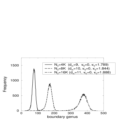
Figure 6: Genus distributions of the mother boundary surface in the strong coupling phase for various sizes.

3.3 Coordination number distributions of boundary surfaces

We must look more carefully into these boundary mfds. In the last few years, several articles have been devoted to the study of boundary mfds. In two dimensions, it is revealed by ref.[13] that the dynamics of the string world sheet (random surfaces) can be described by the time evolution of boundary loops. Furthermore, the work[14] is also based on the idea that the functional integral for $3$ and $4$D quantum gravity can be represented as a superposition of less complicated theory of random surfaces . It is precisely on such grounds that we claim that the higher dimensional complicated theory of quantum gravity can be reduced to the lower dimensional quantum gravity.

The question is that the closed and orientable two-dimensional boundary surfaces mentioned above can be recognized as the two-dimensional random surfaces described by the matrix model or the Liouville field theory. In this subsection, we focus on the distributions of the coordination numbers. The distributions of the coordination numbers have been calculated in ref.[15]. The probability distribution $P_{N}(q)$ can be extracted from the Green functions of the $\phi^{3}$ planar theory with spherical ($S^{2}$) topology without self-energy and tadpole graph in dual lattice,

$$P_{N\to\infty}(q)=16(\frac{3}{16})^{q}\frac{(q-2)(2q-2)!}{q!(q-1)!}\stackrel{{\scriptstyle q\to\infty}}{{\longrightarrow}}e^{-\ln{\frac{4}{3}}q},$$ (6)

where N is a number of 2-simplexes and q is the coordination number. The probability distribution $P_{N}(q)$ with small $q$ region is strongly dependent on the local lattice structures. The value ($\ln{\frac{4}{3}}$) guarantees the randomness of the lattice (see Appendix A). In the preceding subsection we pointed out that spherical mother boundary surfaces whose volumes were greater than $V_{cut}$ had to be considered. Fig.7 shows the (correct-normalized) coordination number distributions of the spherical mother boundary surface for various volumes with $V_{cut}=200$. In Fig.7 we also show the result obtained by the theoretical calculation eq.(6) (broken line).

Figure 7: Normalized coordination number distributions for the mother boundary universe near to the critical point with $N_{3}=8K(\kappa_{0}=3.950$ and $\kappa_{3}=2.165),16K(\kappa_{0}=4.090$ and $\kappa_{3}=2.200)$ and $32K(\kappa_{0}=4.195$ and $\kappa_{3}=2.222)$ with linear-log scales and with $V_{cut}=200$. We have measured the distributions only for the mother boundary surfaces with spherical ($S^{2}$) topology. Broken line is a guide line and denotes the asymptotic scaling relation: $P_{N_{3}}(q)\propto e^{-\ln{\frac{4}{3}}q}$.

The data of the coordination number distributions of the spherical mother boundary surfaces become consistent with the distributions $P_{N}(q)\propto e^{-\ln{\frac{4}{3}}q}$ for large enough $q$. On the other hand, there are a few discrepancies between the two-dimensional theoretical curve and the small $q$ ($q<\sim 25$) distributions in our simulation sizes. We cannot say from only these data whether the mother boundary surfaces with $S^{2}$ topology are equivalent to the random surfaces implemented by the matrix model or not. Further discussion will be presented in the next section.

4 Summary and Discussion

We investigate the boundary surfaces of three-dimensional DT manifolds with $S^{3}$ topology. It have been naively expected that the genus distributions of boundary surfaces will show the scaling properties near the critical point and, in fact, we find scaling behavior, $P(g)\sim g^{-\alpha},$ where $\alpha$ is about $0.5$ in our simulation sizes. On these grounds we may conclude that the thermodynamic limit ($N_{3}\to\infty$) can be taken in this scaling region.

At the strong coupling limit ($\kappa_{0}=0$) the genus distribution of mother universe seems to Gaussian distribution, and it is non-universal in the sense that the peak value of genus $g_{p}$ diverges as $N_{3}\to\infty$.

On the other hand, in the weak coupling region, all of the size of the boundary surfaces are very small, $\sim{\cal O}(1)$, and then these genuses are strongly restricted to zero (i.e., sphere). As a result, there is no scaling behaviour of the genus distributions in the weak coupling phase.

Our numerical results show that the coordination number distributions of the spherical mother boundary surfaces of three-dimensional DT manifolds are consistent with the theoretical prediction in the large $q$ region. When these boundary surfaces can be recognized as surfaces of the matrix model or the Liouville theory, three-dimensional DT manifolds can be reconstructed by the direct products of $\Sigma$ (two-dimensional DT surfaces) and $d$ (geodesic distance). In order to confirm the equivalence between the boundary surfaces in three-dimensions and random surfaces in two-dimensions the string susceptibility $\gamma_{str}$ of the boundary surfaces or the loop-length-distributions (LLD) of the boundary surfaces must be measured and compared with theoretical predictions. We have obtained some preliminary results of the string susceptibility exponents of the boundary surfaces, and a more complete numerical analysis will be published elsewhere.

We will be able to apply our numerical analysis to other physical process such as the topology changing of surfaces of $(2+1)$-dimensional gravity. In this process we substitute the geodesic distance ($d$) for the time, and the two-dimensional surfaces are recognized as the boundary of three-dimensional Euclidean manifold.

Furthermore, the boundary surfaces of three dimensions in general have other nontrivial structures such as Hopf’s link and the nontrivial knot in the knot theory. Up to now, it is difficult to extract the informations for the extrinsic geometry, i.e., how to embed the boundary surface into R³ because we have only intrinsic geometries of DT manifold. To know a mechanism of the formation of nontrivial links or knots is one of challenging subjects in the statistical mechanics.

Appendix A

We can obtain the asymptotic coordination number distribution: eq.(6) only assuming the Poisson distribution function as follows,

$$P(q)\sim e^{-\sigma q}.$$

By using this and the lower limit of $q>3$ we can calculate an average coordination number $<q>$

$$<q>=\frac{\sum qe^{-\sigma q}}{\sum e^{-\sigma q}}=-\frac{d}{d\sigma}\ln{(\sum_{q>3}e^{-\sigma q})}\stackrel{{\scriptstyle N_{0}\to\infty}}{{\longrightarrow}}3+\frac{e^{-\sigma}}{1-e^{-\sigma}}$$

On the other hand, $<q>$ is trivial in two dimensional DT mfd,

$$<q>=\frac{2N_{1}}{N_{0}}=6-\frac{\chi}{N_{0}}\approx 6,$$

where $\chi$ is the Euler number. From eqs.(A.2) and (A.3) we obtain $\sigma=\ln{\frac{4}{3}}$ [16].

Acknowledgements

We are grateful to H.Kawai, T.Yukawa, H.Hagura and T.Izubuchi for useful discussions and comments. One of the authors (N.T.) is supported by Research Fellowships of the Japan Society for the Promotion of Science for Young Scientists.

References

- [1] E.Brézin and V.Kazakov, Phys.Lett. 236B (1990) 144; M.Douglas and S.Shenker, Nucl.Phys. B335 (1990) 635; D.Gross and A.Migdal, Phys.Rev.Lett. 64 (1990) 127.
- [2] V.G.Knizhnik, A.M.Polyakov and A.B.Zamolodchikov, Mod.Phys.Lett A, Vol.3 (1988) 819; J.Distler and H.Kawai, Nucl.Phys. B321 (1989) 509. F.David, Mod.Phys.Lett. A3 (1988) 1651.
- [3] D.Weingarten, Nucl.Phys. B210 (1982) 229; F.David, Nucl.Phys. B257[FS14] (1985) 45; V.A.Kazakov, Phys.Lett. B150 (1985) 282; J.Ambjørn, B.Durhuus and J.Frhlich, Nucl.Phys.B257[FS14] (1985) 433; Nucl.Phys.B275 [FS17] (1986) 161; M.E.Agishtein and A.A.Migdal, Nucl.Phys. B350 (1991) 690.
- [4] H.Kawai and M.Ninomiya, Nucl.Phys. B336 (1990) 115; N.Kawamoto, V.Kazakov, Y.Saeki and Watabiki, Phys.Rev.Lett. 68 (1992) 2113. N.Tsuda and T.Yukawa, Phys.Lett. B305 (1993) 223; H.Kawai, N.Kawamoto, T.Mogami, and Y.Watabiki, Phys.Lett. B306 (1993) 19; Y.Watabiki, Nucl.Phys.B 441 (1995) 119; J.Ambjørn, J.Jurkiewicz and Y.Watabiki, Nucl.Phys.B 454 (1995) 313.
- [5] J.Ambjørn,and S.Varsted, Phys.Lett.B 266 (1991) 285; J Ambjørn, B.Durhuus and T.Jonsson, Mod.Phys.Lett.A 6 (1991) 1133; M.E.Agishtein and A.A.Migdal, Mod.Phys.Lett.A 6 (1991) 1863; D.V.Boulatov and A.Krzywicki, Mod.Phys.Lett.A 6 (1991) 3005; S.Varsted, Nucl.Phys.B (Proc.Suppl.) 26 (1992) 578; S.Catterall, J.Kogut and R.Renken, Phys.Lett.B 342 (1995) 53.
- [6] S.Catterall, J.Kogut and R.Renken, Nucl.Phys.B (Proc.Suppl.) 30 (1993) 775; J.Ambjørn, Z.Burda, J.Jurkiewicz and C.F.Kristjansen, Nucl.Phys.B (Proc.Suppl.) 30 (1993) 771; J.Ambjørn,and S.Varsted, Nucl.Phys.B 373 (1992) 557; J.Ambjørn, D.V.Boulatov, A.Krzywicki and S.Varsted, Phys.Lett.B 276 (1992) 432.
- [7] B.V.de Bakker, Phys.Lett.B 389 (1996) 238; S.Bilke, Z.Burda, A.Krzywicki, B.Petersson, Nucl.Phys.B (Proc.Suppl.) 53 (1997) 743; P.Bialas, Z.Burda, A.Krzywicki, B.Petersson, Nucl.Phys.B 472 (1996) 293
- [8] H.Hagura, N.Tsuda and T.Yukawa, hep-lat/9512016, to be published in Phys.Lett. B.
- [9] B.V.Bakker and J.Smit, Nucl.Phys.B 439 (1995) 239; J.Ambjørn and J.Jurkiewicz, Nucl.Phys.B 451 (1995) 643; I.Antoniadis, P.O.Mazur and E.Mottola, Phys.Lett.B 323 (1994) 284.
- [10] H.S.Egawa, T.Hotta, T.Izubuchi, N.Tsuda and T.Yukawa, Prog.Theor.Phys. 97 (1997) 539; Nucl.Phys.B (Proc.Suppl.) 53 (1997) 760;
- [11] Y.Fujiwara, S.Higuchi, A.Hosoya, T.Mishima and M.Siino, Phys.Rev.D 44 (1991) 1756; Phys.Rev.D 44 (1991) 1763.
- [12] T.Izubuchi, Ph.D.Thesis, University of Tokyo, 1996.
- [13] N.Ishibashi and H.Kawai, Phys.Lett. B314 (1993) 190.
- [14] G.K.Savvidy and K.G.Savvidy, Mod.Phys.Lett. A11 (1997) 1379.
- [15] E.Brézin, C.Itzykson, G.Parisi and J.B.Zuber, Comm.Math.Phys. 59 (1978) 35; D.V.Boulatov, V.A.Kazakov, I.K.Kostov and A.A.Migdal, Nucl.Phys.B 275[FS17] (1986) 641.
- [16] N.Tsuda, Ph.D.Thesis, Tokyo Institute of Technology, 1994.