Logarithmic Corrections to the Equation of State in the SU(2)$\otimes$SU(2) Nambu – Jona-Lasinio Model

Abstract

We present results from a Monte Carlo simulation of the Nambu – Jona-Lasinio model, with continuous $\mbox{SU(2)}\otimes\mbox{SU(2)}$ chiral symmetry, in four Euclidean dimensions. Different model equations of state, corresponding to different theoretical scenarios, are tested against the order parameter data. The results are sensitive to necessary assumptions about the shape and extent of the scaling region. Our best fits favour a trivial scenario in which the logarithmic corrections are qualitatively similar to those predicted by the large $N_{f}$ approximation. This is supported by a separate analysis of finite volume corrections for data taken directly in the chiral limit.

I Introduction

The Nambu – Jona-Lasinio (NJL) model [1] is a quantum field theory of fermions in which the only interaction is an attractive contact interaction between fermion and anti-fermion. Its Lagrangian density is

$${\cal L}=\bar{\psi}_{\alpha p}(\partial{\!\!\!/}\,+m)\psi_{\alpha p}-{g^{2}\over{2N_{f}}}\left[(\bar{\psi}_{\alpha p}\psi_{\alpha p})^{2}-(\bar{\psi}_{\alpha p}\gamma_{5}\vec{\tau}_{pq}\psi_{\alpha q})^{2}\right],$$ (1)

where $\vec{\tau}_{pq}$ are Pauli spin matrices with indices $p,q$ running over an SU(2) internal symmetry, and $\alpha$ runs over $N_{f}$ distinct fermion flavors. For bare mass $m=0$ there is an $\mbox{SU(2)}\otimes\mbox{SU(2)}$ chiral symmetry

$$\psi_{L}\mapsto U\psi_{L}\;\;\;;\;\;\;\psi_{R}\mapsto V\psi_{R},$$ (2)

where $U$ and $V$ are independent global SU(2) rotations. The original motivation for studying the model (1) is that for coupling $g^{2}$ larger than some critical $g_{c}^{2}$ it gives a qualitatively good description of dynamical chiral symmetry breaking in strong interaction physics, with order parameter $\Sigma\propto\langle\bar{\psi}\psi\rangle$. At the large coupling strengths required for chiral symmetry breaking, the fermions interact by exchange of composite scalars and pseudoscalars. In the chiral limit the pseudoscalars are Goldstone modes, and are associated with physical pions. More recently, NJL models have been proposed as a description of the Higgs sector of the standard model [2], in which the Higgs scalar appears as a fermion – anti-fermion bound state, and the Goldstone modes are absorbed into longitudinal gauge boson degrees of freedom.

In weak coupling perturbation theory (WCPT), the NJL model is non-renormalisable for $d>2$, being plagued by quadratic divergences in four dimensions. However, a perturbative expansion made about the critical point $g^{2}=g_{c}^{2}$ in powers of $1/N_{f}$ is known to be renormalisable for $2<d<4$ [3][4], and in $d=4$ suffers from only logarithmic divergences, implying that a moderate separation between UV and IR scales can be made. Because the UV scale can never be completely eliminated from the theory by renormalisation without rendering the interaction strength vanishing, the model is trivial for $d=4$; it shares this property with the model more conventionally used to describe the Higgs sector, namely the O(4) linear sigma model, which contains elementary scalar fields. Both models are believed trivial, and hence provide effective field theories only for scales $\ll\Lambda$, the UV scale. At scales $\sim\Lambda$, logarithmic scaling violations will manifest themselves, which in turn necessitate the introduction of higher dimensional operators corresponding to new physical information. Taking these new operators into account, then in the sense that the number of undetermined parameters is the same for both NJL and sigma models, the two models have equal predictive power for the standard model [5].

If we formulate definite lattice (ie. bare) actions based on these models, however, an approach perhaps more familiar in condensed matter physics, then triviality may manifest itself in distinct ways. For both models the upper critical dimension is four, ie. the symmetry breaking transition is described by mean-field (Landau-Ginzburg) critical exponents with logarithmic corrections. In the sigma model, deviations from mean field behaviour are well-described by WCPT, since the renormalised coupling is bounded by the fixed point value $g_{R}=O(4-d)$ and is small as $d\to 4$. Using the renormalisation group [6][7], the following prediction for the equation of state, relating the order parameter $\Sigma$ to the reduced coupling $t={1\over g^{2}}-{1\over g_{c}^{2}}$ and the symmetry-breaking field $m$ (we retain the notation of the NJL model) is derived:

$$m=At{\Sigma\over{\ln^{1\over 2}\left({1\over\Sigma}\right)}}+B{\Sigma^{3}\over{\ln\left({1\over\Sigma}\right)}}.$$ (3)

Note that $\Sigma$ is measured in units of the cutoff, so that the argument of the logarithms diverges in the continuum limit. By contrast, symmetry breaking in the NJL model occurs for large coupling strength, and WCPT is inapplicable. An alternative expansion parameter, $1/N_{f}$, can be used [8]; at leading order this yields a qualitatively different form for the equation of state [9]

$$m=At\Sigma+B\Sigma^{3}\ln\left({1\over\Sigma}\right).$$ (4)

The different behaviour can be traced to the fact that in the sigma model the scalar excitations are elementary, and the associated wavefunction renormalisation constant $Z$ perturbatively close to one, whereas in the NJL model the scalars are composite, so that $Z$ vanishes in the continuum limit for $d<4$ where the model is renormalisable, and $Z\propto 1/\ln({1\over\Sigma})$ for $d=4$ [8][9]; hence we expect (4) to hold beyond leading order in $1/N_{f}$.

The form (3) in the sigma and related scalar models has been subject to extensive analysis via Monte Carlo simulation (two recent examples are refs.[10][11]), which appear to provide support, although logarithmic corrections are notoriously hard to isolate numerically. For the fermionic case, a simulation of the $d=4$ Gross-Neveu model, with discrete chiral symmetry, has shown support for the form (4) [12]. The issue of which is the appropriate equation of state is important for several reasons; for instance, it informs the study of the inherently non-perturbative chiral symmetry breaking transition in lattice $\mbox{QED}_{4}$. Some studies [13][14] have assumed a scenario of triviality for this model based on a form similar to (3), which may not be appropriate. Another possibility is that different lattice implementations of the chirally symmetric four-fermi interaction, namely the “dual site” formulation [15] used in [12] and in this study, and the “link” formulation used in a Monte Carlo study of the U(1) NJL model in [16], may lie in different universality classes with distinct patterns of logarithmic scaling violations. Studies of the corresponding lattice models in three spacetime dimensions (“dual site” in [4] and “link” in [17]), in which the two implementations yield radically different behaviour, support this scenario.

In this paper we extend the work of [12] with a numerical simulation of the $\mbox{SU(2)}\otimes\mbox{SU(2)}$ NJL model, for a small number of flavors $N_{f}=2$. The main motivation for this choice of four-fermi model, apart from the phenomenological reasons cited above, is that it has a maximal number of Goldstone excitations, all of which contribute to the $O(1/N_{f})$ quantum corrections to the equation of state. We hope to discriminate between the two forms (3) and (4), and in particular to see if (4) persists beyond leading order in $1/N_{f}$. In Sec. II we outline the lattice formulation of (1) using staggered fermions, and discuss its interpretation in terms of continuum four-component spinors. It turns out that in our simulation each lattice species describes eight continuum flavors, and hence the $N_{f}=2$ model requires $N={1\over 4}$ lattice flavors. This necessitates the use of a hybrid molecular dynamics algorithm [18][19]. Extensive studies on small systems reveal the systematic error in the algorithm to be $O(N^{2}\Delta\tau^{2})$, where $\Delta\tau$ is the timestep used in the evolution of the hybrid equations of motion; hence the systematic error can be kept under control. Of course, we are still left with an unquantified error due to the use of a fractional $N$, which implies a non-local action, but have no reason to suspect there is a problem.

In Sec. III we confront data taken on a $16^{4}$ lattice with a range of bare mass values in the critical region $1/g^{2}\simeq 0.5$, with five prototype equations of state reflecting various theoretical prejudices, including the simplest mean field ansatz, and a non-trivial continuum limit described by non-mean field critical indices, as well as (3) and (4). No form satisfactorily fits all the data; this is because there is a finite scaling window where the correlation length is sufficiently large for a continuum description to apply. We show that the most successful equation of state ansatz, in the sense of small $\chi^{2}$, depends on which assumptions are made about the extent of the scaling window: if we include all mass values from a narrow region about the critical coupling then forms similar to (3) are the most successful, whereas if only small mass values from a wide range of couplings are used, then (4) is the most appropriate form.

In Sec. IV we examine data taken at vanishing bare mass, which is possible in four-fermi models formulated via the dual-site approach. Due to the masslessness of the pion in this limit the data is subject to a significant finite volume effect, which we attempt to account for using a formula first derived for the sigma model [11]. We find that the variation of the finite volume correction with $g^{2}$ can best be explained by assuming an equation of state (4), together with a wavefunction renormalisation constant $Z\propto 1/\ln\left({1\over\Sigma}\right)$: in other words, it is the finite volume corrections that seem most sensitive to the composite nature of the scalar excitations. The distinct triviality scenarios in NJL and sigma models [9][12] are rephrased in terms of the pion decay constant $f_{\pi}$. In Sec. V we present brief conclusions and directions for further work.

II Lattice Formulation of the Model

The lattice action we have chosen to study is written

$$S_{bos}=\sum_{\alpha=1}^{N}\sum_{xy}\Psi_{\alpha}^{\dagger}(x)(M^{\dagger}M)^{-1}_{xy}\Psi_{\alpha}(y)+{{2N}\over g^{2}}\sum_{\tilde{x}}\left(\sigma^{2}({\tilde{x}})+\vec{\pi}({\tilde{x}}).\vec{\pi}({\tilde{x}})\right),$$ (5)

where $\Psi_{\alpha}$ are bosonic pseudofermion fields defined in the fundamental representation of SU(2) on lattice sites $x$, the scalar field $\sigma$ and pseudoscalar triplet $\vec{\pi}$ are defined on the dual lattice sites $\tilde{x}$, and the index $\alpha$ runs over $N$ species of pseudofermion; the relation between $N$ and the number of continuum flavors $N_{f}$ will be made clear presently. The fermion kinetic matrix $M$ is the usual one for Gross-Neveu models with staggered lattice fermions [15][4], amended to incorporate an $\mbox{SU(2)}\otimes\mbox{SU(2)}$ chiral symmetry:

$$M_{xy}=\left({1\over 2}\sum_{\mu}\eta_{\mu}(x)[\delta_{y,x+\hat{\mu}}-\delta_{y,x-\hat{\mu}}]+m\delta_{xy}\right)\delta_{\alpha\beta}\delta_{pq}+{1\over 16}\delta_{xy}\delta_{\alpha\beta}\sum_{\langle\tilde{x},x\rangle}\Biggl{(}\sigma(\tilde{x})+i\varepsilon(x)\vec{\pi}(\tilde{x}).\vec{\tau}_{pq}\Biggr{)},$$ (6)

where $m$ is the bare fermion mass, the SU(2) indices $p,q$ are shown explicitly, $\varepsilon(x)\equiv(-1)^{x_{1}+x_{2}+x_{3}+x_{4}}$, and the symbol $\langle\tilde{x},x\rangle$ denotes the set of 16 dual sites $\tilde{x}$ adjacent to the direct lattice site $x$. The 3 Pauli matrices $\tau^{i}$ are normalised such that ${\rm tr}(\tau^{i}\tau^{j})=2\delta^{ij}$.

Integration over the pseudofermions yields the following path integral:

$$Z\propto\int D\sigma D\vec{\pi}\;{\rm det}^{N}(M^{\dagger}M)\exp\left(-{{2N}\over g^{2}}\sum_{x}(\sigma^{2}+\vec{\pi}.\vec{\pi})\right).$$ (7)

In terms of Grassmann fermion fields $\chi,\bar{\chi},\zeta,\bar{\zeta}$, $Z$ can be derived from the equivalent action

$$S=\sum_{\alpha}\left(\bar{\chi}_{\alpha}M[\sigma,\vec{\pi}]\chi_{\alpha}+\bar{\zeta}_{\alpha}M^{\dagger}[\sigma,\vec{\pi}]\zeta_{\alpha}\right)+{{2N}\over g^{2}}\sum_{x}(\sigma^{2}+\vec{\pi}.\vec{\pi}).$$ (8)

The auxiliary fields $\sigma$ and $\vec{\pi}$ can then be integrated out to yield an action written completely in terms of fermion fields:

$$S_{fer} = \sum_{\alpha}\sum_{xy}\bar{\chi}_{\alpha}(x)(\partial{\!\!\!/}\,+m)_{xy}\chi_{\alpha}(y)$$ (11)

$$-{g^{2}\over{8N}}\sum_{\tilde{x}}\left[\left({1\over 16}\sum_{\alpha}\sum_{\langle x,\tilde{x}\rangle}\bar{\chi}_{\alpha}(x)\chi_{\alpha}(x)\right)^{2}-\sum_{i=1}^{3}\left({1\over 16}\sum_{\alpha}\sum_{\langle x,\tilde{x}\rangle}\bar{\chi}_{\alpha}(x)\varepsilon(x)\vec{\tau}\chi_{\alpha}(x)\right)^{2}\right]$$

$$+(\chi\mapsto\zeta;\;\bar{\chi}\mapsto\bar{\zeta};\;\partial{\!\!\!/}\,\mapsto-\partial{\!\!\!/}\,),$$

with $\partial{\!\!\!/}\,_{xy}$ a shorthand for the free kinetic term for staggered lattice fermions. So, we see that the action (5) describes $2N$ flavors of lattice fermion, but with a flavor symmetry group ${\rm U}(N)\otimes{\rm U}(N)$. The interaction term in (8,11) has been normalised so that the gap equation coming from the leading order $1/N$ approximation agrees with that derived for lattice Gross-Neveu models having ${\rm Z}_{2}$ [4] or U(1) [20] chiral symmetries.

Next we identify the global SU(2)$\otimes$SU(2) chiral symmetry of the lattice model. This is most manifest in the form (8). Let ${\cal P}_{e}(x),{\cal P}_{o}(x)$ be even and odd site projectors defined by

$${\cal P}_{e/o}(x)={1\over 2}(1\pm\varepsilon(x)).$$ (12)

Then, noting that ${\cal P}_{e}\partial{\!\!\!/}\,{\cal P}_{o}={\cal P}_{e}\partial{\!\!\!/}\,$ etc, we find that (8) is invariant, in the chiral limit $m\to 0$, under the combined transformation:

$$\chi\mapsto({\cal P}_{e}U+{\cal P}_{o}V)\chi\; \;\bar{\chi}\mapsto\bar{\chi}({\cal P}_{e}V^{\dagger}+{\cal P}_{o}U^{\dagger})$$ ; (13)

$$\zeta\mapsto({\cal P}_{e}V+{\cal P}_{o}U)\zeta\; \;\bar{\zeta}\mapsto\bar{\zeta}({\cal P}_{e}U^{\dagger}+{\cal P}_{o}V^{\dagger})$$ ; (14)

$$\Phi\equiv(\sigma 1\kern-4.5pt1+i\vec{\pi}.\vec{\tau}) \mapsto V\Phi U^{\dagger},$$ (15)

where $U,V$ are independent SU(2) rotations. Note that (15) is a symmetry because $\Phi$ is proportional to a SU(2) matrix, and the auxiliary potential proportional to ${\rm tr}\Phi^{\dagger}\Phi$. This property does not generalise to larger unitary groups. The symmetry (15) is broken explicitly by a bare fermion mass, and spontaneously by the condensates $\langle\bar{\chi}\chi\rangle,\langle\bar{\zeta}\zeta\rangle$.

Now let us consider the continuum flavor interpretation. It is well known that four-dimensional staggered lattice fermions can be interpreted in terms of four flavors of Dirac fermion, which decouple at tree level in the long-wavelength limit. One way of seeing this is via a transformation to fields $q,\bar{q}$ defined on the sites $y$ of a lattice of spacing $2a$ [21]:

$$q^{\alpha a}(y)={1\over 8}\sum_{A}\Gamma_{A}^{\alpha a}\chi(A;y)\;\;;\;\;\bar{q}^{\beta b}={1\over 8}\sum_{A}\bar{\chi}(A;y)\Gamma_{A}^{*\beta b},$$ (16)

where $\alpha,\beta=1,\ldots,4$ run over spin degrees of freedom, $a,b=1,\ldots,4$ over flavor, and $A$ is a four-vector with entries either 0 or 1 which identifies the corners of the elementary hypercube associated with site $y$; each site $x$ on the original lattice is thus mapped to a unique combination $(A;y)$. The $4\times 4$ matrix $\Gamma_{A}\equiv\gamma_{1}^{A_{1}}\gamma_{2}^{A_{2}}\gamma_{3}^{A_{3}}\gamma_{4}^{A_{4}}$, where $\gamma_{\mu}$ are Dirac matrices. The action written in the form (8) contains interaction terms of the form $\sigma\bar{\chi}\chi$, $\vec{\pi}.\bar{\chi}\vec{\tau}\chi$ etc. In the $q$-basis the $\sigma$ and $\pi$ fields are not all equivalent. If we label the dual site $(x_{1}+{1\over 2},\ldots,x_{4}+{1\over 2})$ by $(A;\tilde{y})$, then for $A=(0,0,0,0)$ the interaction reads

$$S_{int}(0;\tilde{y})=\sigma(0;\tilde{y})\bar{q}(y)(1\kern-4.5pt1\otimes 1\kern-4.5pt1)q(y)+i\vec{\pi}(0;\tilde{y}).\bar{q}(y)\vec{\tau}(\gamma_{5}\otimes\gamma_{5}^{*})q(y),$$ (17)

where the first matrix in the direct product acts on spin degrees of freedom, and the second on flavor. Equation (17) resembles the continuum interaction between fermions and the auxiliary scalars, except that the pseudoscalar current is non-singlet (but diagonalisable) in flavor space. However, for $A_{\mu}=1,A_{\nu\not=\mu}=0$, say, the interaction is more complicated:

$$S_{int}( \mu ;\tilde{y})=\sigma(\mu;\tilde{y})\left[\bar{q}(y)q(y)+{1\over 2}\Delta_{\mu}^{+}\left(\bar{q}(y)q(y)+\bar{q}(y)(\gamma_{\mu}\gamma_{5}\otimes\gamma_{5}^{*}\gamma_{\mu}^{*})q(y)\right)\right]$$ (18)

$$+i\vec{\pi}( \mu ;\tilde{y}).\left[\bar{q}(y)\vec{\tau}(\gamma_{5}\otimes\gamma_{5}^{*})q(y)+{1\over 2}\Delta_{\mu}^{+}\left(\bar{q}(y)\vec{\tau}(\gamma_{5}\otimes\gamma_{5}^{*})q(y)+\bar{q}(y)\vec{\tau}(\gamma_{\mu}\otimes\gamma_{\mu}^{*})q(y)\right)\right],$$ (19)

where $\Delta_{\mu}^{+}$ is the forward difference operator on the $y$-lattice. Hence in addition to continuum-like interactions there are extra momentum-dependent terms coupling the auxiliary fields to bilinears which do not respect Lorentz or flavor covariance. For $A$ vectors with more non-zero entries there are still more complicated interactions containing more derivative terms.

One might naively claim that the terms in $\Delta_{\mu}\sigma,\Delta_{\mu}\pi$ are $O(a)$ and hence irrelevant in the continuum limit. This ignores the fact that $\sigma$ and $\pi$ are auxiliary fields which have no kinetic terms to suppress high momentum modes in the functional integral. The non-covariant terms will thus survive integration over $\sigma,\vec{\pi}$ to manifest themselves in (11). A similar phenomenon happens in lattice formulations of the NJL model in which the interaction term is localised on a single link [16][22]. The effects of the non-covariant terms in fact depend on the details of the model’s dynamics. If long-range correlations develop among the auxiliary fields, ie. if an effective kinetic term is generated by radiative corrections, then the $\Delta_{\mu}\Phi$ term may become irrelevant – this appears to be the case in two [15][23] and three [4] dimensional models, where in each case there is a renormalisable expansion available. In four dimensions the NJL model is trivial: hence no continuum limit exists. Even in this case, though, we expect correlations to develop between the auxiliary fields in the vicinity of the continuous chiral symmetry breaking transition. In this case the unwanted interactions would manifest themselves as scaling violations if an interacting effective theory is to be described [5].

From the arguments following (11) and (16) we now state the relation between the parameter $N$ and the number of continuum flavors $N_{f}$:

$$N_{f}=8N.$$ (20)

The extra factor of 2 over the usual relation for four-dimensional gauge theories arises from the impossibility of even/odd partitioning in the dual site approach to lattice four-fermi models: in other words the matrix $M$ contains diagonal terms which are not multiples of the unit matrix. In this paper we wish to study a small number of continuum flavors $N_{f}=2$, which necessitates a fractional $N=0.25$. This can be achieved using a hybrid algorithm, which produces a sequence of configurations weighted according to the action (7) by Hamiltonian evolution in a fictitious time $\tau$ [18], the fields’ conjugate momenta being stochastically refreshed at intervals. The advantage of this approach is that in the form (7) the variable $N$ can readily be set to a non-integer value (though there is no longer a transformation to a local action of the form (11)); the cost is that the simulation must be run with a discrete timestep $\Delta\tau$. In principle several values of $\Delta\tau$ must be explored, then the limit $\Delta\tau\to 0$ taken. We have chosen to implement the “R-algorithm” of Gottlieb et al [19], for which the systematic error is claimed to be $O(\Delta\tau^{2})$.

We have tested the R-algorithm by extensive runs on a $6^{4}$ lattice with parameters $1/g^{2}=0.56$ and mass $m=0.01$, the coupling being chosen to lie well into the broken symmetry phase according to the leading order gap equation (see below). We tested models with $N=0.25,1,3$ and 6, with timesteps $\Delta\tau=0.4$ (for$N\leq 1$), 0.2, 0.1 and 0.05. For integer $N$ we were also able to run directly in the $\Delta\tau=0$ limit using an exact hybrid Monte Carlo algorithm [24][4]. We ran for either 20000 ($N=3,6$) or 40000 ($N=0.25,1$) Hamiltonian trajectories between momentum refreshments, the trajectory lengths being drawn from a Poisson distribution with mean 1.0.

For illustration we present results for two local quantities, the expectation value of the scalar field $\langle\sigma\rangle\equiv\Sigma$, and the energy density $\epsilon$ given by

$$\epsilon={1\over{2V}}\left\langle\sum_{x}M^{-1}_{x,x+\hat{4}}-M^{-1}_{x,x-\hat{4}}\right\rangle.$$ (21)

The results are shown in Figs. 1 and 2, together with quadratic fits of the form

$$\Sigma(N;\Delta\tau)=\Sigma_{0}(N)+A(N)\Delta\tau^{2}\;\;\;;\;\;\;\epsilon(N;\Delta\tau)=\epsilon_{0}(N)+B(N)\Delta\tau^{2}.$$ (22)

Acceptable fits were found for all datasets except for the $\Sigma$ data at $N=6$, where the fit was restricted to $\Delta\tau\leq 0.1$. We find good evidence that the systematic error is indeed $O(\Delta\tau^{2})$. Moreover, the coefficients $A(N)$ and $B(N)$ are themselves adequately fitted by the forms $A(N)=aN^{2}$, $B(N)=bN^{2}$ as displayed in Fig. 3. This behaviour is expected from inspection of the hybrid equations of motion [18][19].

Since fluctuations in the system are suppressed by powers of $1/N$, we see that for $N=0.25$ systematic errors are likely to be dwarfed by statistical ones for reasonable simulation runs. In the work presented in the rest of this paper we took $\Delta\tau=0.05$ just to be conservative and safe. In fact, for very small or vanishing bare mass $m$ near the critical point where the order parameter is very small, we also did production runs with $\Delta\tau=0.025$ to check explicitly that the systematic errors were smaller than the statistical errors.

The bulk of the results of this paper were generated on a $16^{4}$ lattice with $N=0.25$, using masses $m$ ranging from 0.05 down to 0.0025. We have focussed our attention on the order parameter $\Sigma$, which differs from zero in the chiral limit only when chiral symmetry is spontaneously broken, and is simply related to the chiral condensate: $\Sigma={g^{2}\over 2}\langle\bar{\chi}\chi\rangle$. Our results for $\Sigma$ as a function of bare mass $m$ and inverse coupling $1/g^{2}$ are presented in Tab. I. Because the kinetic matrix $M$ contains numerically large diagonal terms, this model is relatively cheap to simulate compared to, say, non-compact QED. This has enabled us to accumulate a large dataset, reflected in the relatively small statistical errors in Tab. I. Typical runs which resulted in each of the entries in that table were between 15,000 and 30,000 $\tau$ units long. Such statistics are an order of magnitude better than present day state-of-the-art lattice QCD simulations. The statistical error bars in the table were obtained by binning methods which are particularly reliable when applied to such substantial data sets.

In fact, because the interactions appear on the diagonal, $M$ is sufficiently well-conditioned in the broken phase to permit simulations directly in the chiral limit $m=0$. Of course, since spontaneous symmetry breaking cannot occur in a finite volume $V$, $\Sigma$ is strictly zero in these simulations; defining

$$\bar{\Phi}={1\over V}\sum_{x}\Phi(x),$$ (23)

then the next best thing to measure is

$$|\Phi|=\left\langle\sqrt{\textstyle{1\over 2}\mbox{tr}\bar{\Phi}^{\dagger}\bar{\Phi}}\right\rangle.$$ (24)

This quantity is numerically very close to $\Sigma$ extrapolated to the chiral limit, but exceeds it in a finite volume. We will discuss the finite volume correction in more depth in Sec. IV. Our results for $|\Phi|$ are given in Tab. II. To monitor finite volume effects directly we did a small number of runs on $12^{4}$ and $20^{4}$ lattices, and tabulate the results in Tabs. II and III

Finally in this section we give details of the model’s gap equation. In the large-$N$ limit, for sufficiently strong coupling $g^{2}$, the scalar auxiliary $\sigma$ develops a spontaneous vacuum expectation value $\Sigma$ even in the chiral limit $m\to 0$. To leading order in $1/N$ the relation between $\Sigma$, the bare mass $m$ and $g^{2}$ is given by the lattice tadpole or gap equation [4]:

$${1\over g^{2}} = 16{{m+\Sigma}\over{\Sigma}}\int_{-\pi/2}^{\pi/2}{{d^{4}k}\over(2\pi)^{4}}{1\over{\sin^{2}k_{\mu}+(m+\Sigma)^{2}}}$$ (25)

$$= {{m+\Sigma}\over{\Sigma}}\int_{0}^{\infty}d\alpha\exp-\alpha\left(2+(m+\Sigma)^{2}\right)I_{0}^{4}({\alpha\over 2}),$$ (26)

with $I_{0}$ a modified Bessel function. In Fig. 4 we show predictions for $\Sigma$ as a function of $g^{2}$ for $m$ values 0.0, and 0.01. The $m=0$ line shows a continuous transition at $1/g_{c}^{2}\simeq 0.62$ between a symmetric phase at weak coupling and a broken phase at strong coupling – the curve having the $(g^{2}-g_{c}^{2})^{1\over 2}$ shape characteristic of mean field theory. For $m>0$, $\Sigma\not=0$ for all values of $g^{2}$. Also shown are simulation results from a $6^{4}$ lattice with $m=0.01$ for various $N$, showing:

1. that increasing fluctuations, expected to be $\propto 1/N$, cause a suppression of $\Sigma$.

2. that the simulated values of $\Sigma$ exceed the gap equation predictions for $N>3$: this is in marked contrast to the case in three dimensions, where the gap equation gives an upper bound for all $N$ [4]. Perhaps the lack of numerical accuracy of the gap equation is because the $1/N$ expansion is not renormalisable in four dimensions.

III Numerical Fits to the Equation of State

In this section we report on fits to various trial forms for the equation of state $m=f(\Sigma,1/g^{2})$ using data for the order parameter tabulated in Tab. I. We used the numerical package minuit to perform least squares fits, and in each case quote a standard error for the fitted parameters, and the $\chi^{2}$ per degree of freedom, which gives a measure of the quality of the fit.

First we list the functional forms we have examined, in increasing order of sophistication:

1. Mean Field (3 parameters):

   $$m=A\left({1\over g^{2}}-{1\over g_{c}^{2}}\right)\Sigma+B\Sigma^{3}.$$ (27)

   This is the simplest form, arising from a mean field treatment neglecting fluctuations in the order parameter field.

2. Power Law (5 parameters):

   $$m=A\left({1\over g^{2}}-{1\over g_{c}^{2}}\right)\Sigma^{p}+B\Sigma^{\delta}.$$ (28)

   This is a more general version of I, derivable by renormalisation group arguments from the assumption that a fixed point exists at the transition corresponding to a diverging ratio between cutoff and physical scales. A useful discussion is found in [7]. The index $\delta$ is the standard critical exponent, and $p=\delta-1/\beta$, where $\beta$ is another standard exponent.

3. Ladder Approximation (4 parameters):

   $$m=A\left({1\over g^{2}}-{1\over g_{c}^{2}}\right)\Sigma+B\Sigma^{\delta}.$$ (29)

   This is a restricted form of II based on the relation $\gamma\equiv 1\Rightarrow\delta-1/\beta\equiv 1$, inspired by solution of the quenched gauged U(1) NJL model in ladder approximation [25].

The last three fits all assume that the leading behaviour is described by the exponents of mean field theory (ie. $\delta=3$, $p=1$), but with logarithmic scaling corrections. Since these corrections introduce a dependence on some ultraviolet scale, they imply that the renormalised theory near the fixed point can never be made independent of the cutoff, and hence that the continuum limit is described by a free field theory – this is the phenomenon of triviality. The standard scenario is derived using renormalised perturbation theory in the context of $\mbox{O}(n)$ scalar field theory [6][7]. This gives rise to:

1. Sigma Model Logarithmic Corrections (4 parameters):

   $$m=A\left({1\over g^{2}}-{1\over g_{c}^{2}}\right){\Sigma\over{\ln^{1\over 2}\left({C\over\Sigma}\right)}}+B{\Sigma^{3}\over{\ln\left({C\over\Sigma}\right)}}.$$ (30)

   Here the powers of the logarithmic terms are derived on the assumption that the effective field theory at the fixed point is the O(4) linear sigma model, which has the same pattern of symmetry breaking as our SU(2)$\otimes$SU(2) model. Note that we include $C$, the UV scale of the logarithm, as a free parameter. Since the condensate data are measured in lattice units, we expect a plausible fit should have $C$ of $O(1)$.

2. Modified Sigma Model Logarithmic Corrections (5 parameters):

   $$m=A\left({1\over g^{2}}-{1\over g_{c}^{2}}\right){\Sigma\over{\ln^{q_{1}}\left({1\over\Sigma}\right)}}+B{\Sigma^{3}\over{\ln^{q_{2}}\left({1\over\Sigma}\right)}}.$$ (31)

   Here we allow the powers of the logarithms to vary. This phenomenological form has been used extensively in fits of the equation of state of both non-compact lattice QED [13][14] and the U(1) NJL model [16]. Note that we have set the UV scale in the logarithm to 1; fits in which both $p$ and $C$ are allowed to vary are inherently unstable, since $\ln(C/\Sigma)=\mbox{const.}+\ln^{1/\ln C}(1/\Sigma)$, so that as $\Sigma\to 0$ the functional forms become so similar that the covariance matrix becomes singular.

3. Large-$N$ Logarithmic Corrections (4 parameters):

   $$m=A\left({1\over g^{2}}-{1\over g_{c}^{2}}\right)\Sigma+B\Sigma^{3}\ln\left({C\over\Sigma}\right).$$ (32)

   This form is predicted for the NJL model in the large-$N$ limit [9], and was used to fit data from the four dimensional $\mbox{Z}_{2}$ NJL model in [12]. There are important qualitative differences between form VI and the previous forms IV, V, due to the different role of the logarithmic term – i.e. the “effective” value of the exponent $\delta$ measured at the critical coupling is larger than the mean field value 3 for IV and V, but smaller than 3 for fit VI.

We also tried to fit slightly modified forms of IV – VI, eg, allowing separate scales in the logarithms, but the results were either unstable, or not sufficiently distinct from the six forms presented here to be worth reporting.

As we shall see, the main issue to arise when assessing the various forms (27-32) is how much of the data to include in the fit. We expect any fit only to be successful in some finite scaling region around the transition. To see this, consider fits using all 84 data points, shown in Tab. IV. No fit gives acceptable results as judged by the large $\chi^{2}$, although the two 5 parameter forms II and V are both noticeably better. To proceed, we must make some assumptions about the size and shape of the scaling window in the $(1/g^{2},m)$ plane, and truncate the dataset accordingly. In Tab. V we exclude extremal inverse coupling values and fit to $1/g^{2}\in[0.52,0.55]$, which still includes over half the data in the set. The resulting fits fall into two camps. Forms I, III and VI all yield similar large $\chi^{2}$ and $1/g_{c}^{2}$, and are all in effect forced very close to the mean field form $\delta=3$, $p=1$; in the case of VI by having the UV scale so large that the logarithmic term is effectively constant. These fits all fail because the data in this window does not favour $p=1$. Forms II, V and to a lesser extent IV all allow the effective $p$ to increase from 1, e.g. for form V $p_{eff}=1+q_{1}/\ln({1\over\Sigma})>1$. This enables better fits, which are also characterised by a smaller value for $1/g_{c}^{2}$; to see why consider a Fisher plot of the data, in which $\Sigma^{2}$ is plotted against $m/\Sigma$. The Fisher plot is designed so that the mean field equation of state (27) yields curves of constant $1/g^{2}$ which are straight lines of uniform slope, intercepting the vertical axis as $m\to 0$ in the broken phase, the horizontal axis as $m\to 0$ in the symmetric phase, and passing through the origin as $m\to 0$ for $g^{2}=g_{c}^{2}$. Any departures from mean field behaviour show up as curvature in and variation in spacing between lines of uniformly spaced values of $1/g^{2}$.

In Fig. 5 we plot lines of constant $1/g^{2}$ using III, showing that the lines are straight and make a poor job of passing through the data points. The plots from I and IV are almost indistinguishable. In Fig.6 we show the same plot for II, and in Fig. 7 the plot for V. These last two fits are relatively successful because they accommodate lines of constant $1/g^{2}$ whose curvature changes sign according to which phase one is in.

Outside the fitted window form II copes slightly better in the broken phase. It is worth noting that forms II and V gave fits of similar quality when applied both to simulation results of both the U(1) NJL model [16] and non-compact QED [14]; clearly the logarithmic correction of (31) can equally well be modelled by an effective $\delta>3$. We have checked that fits II and V were stable under exclusion of $1/g^{2}=0.52,0.55$, and also under exclusion of the low mass points $m=0.005,0.0025$.

A study of Figs. 6,7 however, indicates that fits II and V are least satisfactory for the low mass points closest to the origin. This has led us to explore an alternative scaling window, in which all $1/g^{2}$ values are kept, but high mass points are excluded. Results from just keeping the 29 points corresponding to $m=0.0025,0.005$ are given in Tab. VI, and those for the 40 points obtained by also including $m=0.01$ in Tab. VII. The picture changes dramatically: the $\chi^{2}$ values from fits III and VI are now much smaller and comparable to those from fits II and V, though for $m\leq 0.005$ (Tab. VI) the two 5 parameter fits still yield the lowest values. Once $m=0.01$ points are included, fits II, III, V and VI are virtually indistinguishable in quality.

What has happened is that the data from this window prefer an effective value of $p$ much closer to 1, and an effective $\delta$ now less than 3. This results, e.g. in the value of $q_{1}$ in fit V being very small, almost consistent with zero. The most impressive effect is that the logarithmic correction of form VI is now acting in the correct way to fit the data, moreover with a reasonable value for the UV scale $C$: in fit V this manifests itself in a relatively large negative value for the exponent $q_{2}$. The form IV, which assigns a positive value to $q_{2}$, is unstable.

In Figs. 8 and 9 we show Fisher plots for the forms II and VI respectively, using the fit parameters of Tab. VII, showing that the fits are indeed successful over a wide range of $1/g^{2}$ at the expense of missing the higher mass points. The even spacing of the lines of constant $1/g^{2}$ in the broken phase is responsible for forcing the effective value of $p$ to one.

The values of $\chi^{2}$ per degree of freedom for the four successful fits are slightly too high for us to claim that they are the last word on understanding the model’s equation of state. Even though the fits reproduce the spacing of the data in $1/g^{2}$, close inspection of Figs. 8 and 9 suggests that the variation of the data with $m$ in the broken phase is not so well-described – clearly more low mass data will be needed to settle the issue, which in turn will require a quantitative understanding of finite volume corrections. We can claim, however, that there appears to be a dramatic switch in the preferred form of the equation of state according to whether the scaling window is chosen long and thin or short and fat in the $(1/g^{2},m)$ plane. In the next section we will consider data taken directly in the chiral limit, and find indirect evidence to support the short fat option.

IV Finite Volume Corrections in the Chiral Limit

In the previous section we made no attempt to correct for finite volume effects in the measurements of $\Sigma$. From test runs for $m=0.005$ at $1/g^{2}=0.50$ on different-sized lattices, shown in Tab. III, finite volume effects are clearly present on a $12^{4}$ system, but the difference between $16^{4}$ and $20^{4}$, though statistically significant, is less than 2%. We hope, therefore, that finite volume corrections would have no impact on the qualitative conclusions of the previous section.

Finite volume effects are numerically important, however, when considering measurements of the quantity $|\Phi|$ made with $m=0$, defined in (24) and shown in Tab. II. Naively, we expect that in a finite system $|\Phi|$ differs from the true order parameter $\Sigma$ extrapolated to the chiral limit, because in the absence of a symmetry breaking term it is impossible to disentangle fluctuations of the order parameter field from those of the Goldstone modes; including the effects of the latter will give $|\Phi|>\Sigma_{0}$, where $\Sigma_{0}$ denotes the value of $\Sigma$ in the chiral limit. Only in the thermodynamic limit $V\to\infty$ do we expect the Goldstone modes to average to zero and the two quantities to coincide. This phenomenon also occurs in numerical studies of scalar field theory, and has been analysed for the O(4) sigma model in [11]. Formally, $|\Phi|$ corresponds to the minimum of a “constraint effective potential” in a finite volume $V$; for the O(4) sigma model this can be calculated using renormalised perturbation theory. There is indeed a correction due to the Goldstone modes which is intrinsically $O(V^{-1})$. Numerically, however, a far more significant correction to the calculation arises from the need to renormalise the model in order to relate lattice parameters to measured quantities. To one-loop order this results in a relation [11]

$$|\Phi|=\Sigma_{0}\left(1+B(m_{R}L){Z\over{\Sigma_{0}^{2}L^{2}}}+O(g_{R}^{2})\right),$$ (33)

where $m_{R}$, $g_{R}$ are the renormalised scalar mass and coupling strength, $L$ is the linear size of the system, and $Z$ is the wavefunction renormalisation constant, defined as the coefficient of $1/p^{2}$ in the unrenormalised pion propagator in the limit $p^{2}\to 0$. The factor $B$ is a slowly varying function of $m_{R}L$ which accounts for the difference between one-loop integrals evaluated in finite and infinite volumes (for further background see [26]). A fit to (33) for magnetisation data in the sigma model is given in Fig. 2 of [11].

For the NJL model there is no reason for renormalised perturbation theory to apply; however since the effective theory in the broken phase is similar to the sigma model, in the sense that it has the same light scalar degrees of freedom, we expect a result similar to (33) to hold. We will therefore attempt to account for the finite volume correction $\Delta=|\Phi|-\Sigma_{0}$ with the formula

$$\Delta={{BZ}\over{\Sigma_{0}L^{2}}},$$ (34)

where the $B$ factor has been set constant, and higher order effects are ignored.

The first prediction of (34) is that $\Delta\propto L^{-2}$. To test this, we can compare $|\Phi|$ data taken at $1/g^{2}=0.48$ from three different volumes against our best estimate for $\Sigma_{0}$. From the data of Tab. II we see that $|\Phi|$ decreases with $L$ as predicted. To evaluate $\Sigma_{0}$, we use the two most successful fits to the equation of state from the previous section, each one characteristic of the two different hypotheses about the shape of the scaling window. The narrow scaling window $0.52\leq 1/g^{2}\leq 0.55$ was best fitted by form V (31) using the parameters of Tab. V (the corresponding Fisher plot is shown in Fig. 7); in the chiral limit at $1/g^{2}=0.48$ this form predicts $\Sigma_{0}=0.3341$ (we implicitly assume here that the equation of state fits apply to the thermodynamic limit). This is already equal to the value of $|\Phi|$ on a $12^{4}$ lattice, and lies above $|\Phi|$ on larger systems, making it difficult to see how (34) applies. The second estimate comes from assuming a wide scaling window in $1/g^{2}$ but excluding higher mass data. This was best described using form VI (32) using the parameters of Tab. VII (Fig. 9); the chiral limit prediction now is $\Sigma_{0}=0.3030$. In Fig. 10 we plot $({L\over 12})^{n}\Delta$ vs. $1/L$ for $n=1$, 2 and 3 and $L=12$, 16 and 20, assuming $\Sigma_{0}=0.3030$. We find that $L^{2}\Delta$ is approximately constant, which supports the hypothesis (34).

Next we examine the dependence of $\Delta$ on $1/g^{2}$, and hence $\Sigma_{0}$, using data from the broken phase of the model taken from a constant volume of $16^{4}$. The data of Tab II were used in conjunction with the same two fits for $\Sigma_{0}$ to produce the two sets of values for $\Delta$ given in Tab. VIII. The quoted errors are the statistical errors in the measurement of $|\Phi|$, and take no account of errors in extrapolating $\Sigma$ to the chiral limit. The values $\Delta_{\mbox{V}}$ obtained using form V actually change sign over the range of $1/g^{2}$ explored, and clearly cannot be fitted by any relation of the form (34). The values $\Delta_{\mbox{VI}}$ obtained using form VI are plotted against $1/g^{2}$ in Fig. 11. The most interesting trend is that $\Delta_{\mbox{VI}}$ is approximately constant for $0.45\leq 1/g^{2}\leq 0.52$, whereas $\Sigma_{0}$ itself falls from 0.4115 to 0.1332 over the same range.

How do we reconcile this observation with (34), which apparently predicts $\Delta\propto 1/\Sigma_{0}$? The answer lies in the field dependence of the wavefunction renormalisation constant $Z$, which differs markedly between the ferromagnetic O(4) sigma model and the fermionic NJL model [8][9][12]. In the sigma model, $Z$ is perturbatively close to 1 (as borne out by the data of [11]), and hence $\Delta\propto 1/\Sigma_{0}$. In the NJL model, on the other hand, the large-$N_{f}$ approximation predicts $Z\propto 1/\ln(1/\Sigma_{0})$ [8], and hence

$$\Delta\propto{1\over{\Sigma_{0}\ln\left({1\over\Sigma_{0}}\right)}}.$$ (35)

We can see this using another argument. In both sigma and NJL models, a Ward identity plus the assumption that both conserved current and transverse field couple principally to the Goldstone mode (in particle physics this mode is the pion, and the assumption is PCAC), leads to the relation [26]

$$Zf_{\pi}^{2}=\Sigma_{0}^{2},$$ (36)

where $f_{\pi}$ is the coupling to the axial current, or in the context of hadronic physics the pion decay constant. We thus have

$$\Delta\propto{\Sigma_{0}\over{(f_{\pi}L)^{2}}}.$$ (37)

Now, in the large-$N_{f}$ approximation (see Appendix for an explicit calculation),

$$f_{\pi}={{\sqrt{N_{f}}\Sigma_{0}}\over\pi}\ln^{1\over 2}\left({1\over\Sigma_{0}}\right),$$ (38)

yielding once again the relation (35).

Note that both scenarios predict triviality of the resulting theory. In the NJL model, in the large-$N_{f}$ treatment $\Sigma_{0}$ is a physical scale related to the renormalised fermion and scalar masses. The pion decay constant in physical units is thus $f_{\pi}/\Sigma_{0}$, which diverges as $\ln^{1\over 2}(1/\Sigma_{0})$ in the continuum limit $\Sigma_{0}\to 0$. In the sigma model, $f_{\pi}/\Sigma_{0}=Z^{1\over 2}$ which is constant in the continuum limit; however the physical scale is now the scalar mass $m_{\sigma}\propto\surd{g_{R}}\Sigma_{0}$. Hence in physical units

$${{f_{\pi}}\over{m_{\sigma}}}\propto{1\over\surd{g_{R}}}\propto{\ln^{1\over 2}\left({1\over\Sigma_{0}}\right)},$$ (39)

and again diverges in the continuum limit.

We tested the hypothesis (35) with a two parameter fit of the data of Tab. VIII to the form

$$\Delta={A\over{16^{2}\Sigma_{0}\ln\left({B\over\Sigma_{0}}\right)}}.$$ (40)

With all points included we find $A=1.86(13)$, $B=1.10(11)$ with $\chi^{2}/\mbox{dof}$ of 4.3; however if the $1/g^{2}=0.53$ point is left out the fit is much more satisfactory: $A=1.40(10)$, $B=0.82(6)$ with $\chi^{2}/\mbox{dof}$ of 0.81. This fit is plotted in Fig. 11. In either case it is reassuring that the UV scale of the logarithm is close to unity. It is also interesting that the fit accounts for the slight curvature in the plot, though this aspect is not tightly constrained by the current error bars. The fitted curve also rises sharply to pass close to the excluded point.

To conclude, we can account for our finite volume effects in the chiral limit under three assumptions:

1. that the equation of state fits to the $\Sigma$ data from the $16^{4}$ lattice in the previous section, when extrapolated to the chiral limit, accurately describe the thermodynamic limit.

2. that the most appropriate form to extrapolate the equation of state is form VI (32), using the parameters of Tab. VII.

3. that the finite volume correction has the form (35).

The latter two assumptions are consistent with logarithmic corrections of the form advocated in [9], which differ qualitatively from those used to describe triviality in scalar field theory.

V Discussion

It would appear that for the lattice sizes and bare masses used in this study, which are close to state-of-the-art (though recall that dual-site four-fermi models are relatively cheap to simulate), it is still difficult to distinguish different patterns of triviality, or indeed distinguish a trivial from a non-trivial fixed point, purely on the basis of fits to model equations of state; different assumptions about the size and shape of the scaling region result in different best fits. Only once the analysis of Sec. IV is applied to the data taken at zero bare mass does the form (32), associated with composite scalar degrees of freedom, appear preferred. Our principal conclusion is thus that the form (4), (32) is qualitatively correct beyond leading order in the $1/N_{f}$ expansion.

The sensitivity of the preferred form of the equation of state to the shape of the assumed scaling window has implications for similar studies in related fermionic models, noteably the U(1) NJL model studied using the “link” formulation [16], and non-compact $\mbox{QED}_{4}$ [14]; the two recent studies cited attempt fits based on the power law form (28) and the modified sigma model form (31), and find the two forms difficult to distinguish on the basis of $\chi^{2}$ alone (in other words, a value of $\delta>3$ is difficult to distinguish from a logarithmic correction with $q_{2}>0$). In Tab. IX the values of $q_{1}$ and $q_{2}$ are shown for the two scaling windows used in this study, together with the quoted fits for the two other models from [16] and [14], as well as theoretical values for the O(4) and O(2) sigma models [6][7], corresponding respectively to the broken $\mbox{SU(2)}\otimes\mbox{SU(2)}$ symmetry in this study, and the broken U(1) chiral symmetry of the models of [16] and [14]. Using the data of [14] one can examine the stability of the fitted $q_{1}$ and $q_{2}$ with respect to exclusion of higher mass data; the quoted value for $q_{1}$ appears quite stable, that for $q_{2}$ less so.

An outstanding issue is whether the disparity in the fitted values of the $q$ exponents in Tab. IX means that the different lattice models lie in different universality classes. The analysis presented in this paper suggests that current lattice simulations are unable to decide. Unfortunately for the two models considered in [16][14] there is no realisable way of simulating directly in the chiral limit, and hence the analysis of Sec. IV is unavailable. A useful direction to explore may be a simulation of the U(1) NJL model with the dual site formulation.

$1/N_{f}$ Calculation of $f_{\pi}$

In this appendix we calculate the pion decay contant $f_{\pi}$, defined by the PCAC relation

$$\langle 0|A_{\mu}^{\alpha}|\pi^{\alpha}(q)\rangle\equiv\langle 0|\bar{\psi}i\gamma_{\mu}\gamma_{5}{{\tau^{\alpha}}\over 2}\psi|\pi^{\alpha}(q)\rangle=iq_{\mu}f_{\pi},$$ (41)

in the large-$N_{f}$ approximation of the NJL model. Diagrammatically the matrix element to analyse is shown in Fig. 12. Note that the external pion leg yields a normalisation factor $Z^{1\over 2}$, where $Z$ is defined by the infrared limit of the pion propagator $D_{\pi}$:

$$\lim_{q\to 0}D_{\pi}(q)={Z\over q^{2}}.$$ (42)

For $d<4$ $Z$ is finite. In the NJL model to leading order in $1/N_{f}$ it is given by [4]

$$Z={1\over g^{2}}{(4\pi)^{d\over 2}\over{2\Gamma(2-{d\over 2})}}\Sigma^{4-d}.$$ (43)

The matrix element is then given by

$$\langle 0|A_{\mu}^{\alpha}|\pi^{\alpha}(q)\rangle=Z^{1\over 2}N_{f}\times{g\over{2\sqrt{N_{f}}}}\int_{p}\mbox{tr}\left\{{1\over{ip{\!\!\!/}\,+\Sigma}}\gamma_{\mu}\gamma_{5}\tau^{\alpha}{1\over{i(p{\!\!\!/}\,+q{\!\!\!/}\,)+\Sigma}}\gamma_{5}\tau^{\alpha}\right\},$$ (44)

where details of Feynman rules and evaluation of $\int_{p}$ are also given in [4]. For $d<4$ the integral can be evaluated to yield

$$\langle 0|A_{\mu}^{\alpha}|\pi^{\alpha}(q)\rangle=gZ^{1\over 2}\sqrt{N_{f}}\times 4\Sigma iq_{\mu}\times{{\Gamma(2-{d\over 2})}\over{(4\pi)^{d\over 2}}}\int_{0}^{1}dx{1\over{(\Sigma^{2}+x(1-x)q^{2})^{2-{d\over 2}}}}.$$ (45)

We now take the chiral limit $\Sigma^{2}\gg q^{2}$, valid for an on-shell pion; combining this step with relations (41) and (43) we find

$$f_{\pi}=2\surd 2\sqrt{N_{f}}\Sigma^{{d\over 2}-1}\sqrt{\Gamma(2-{d\over 2})\over(4\pi)^{d\over 2}}.$$ (46)

This agrees with the result found for $d=3$ in [27].

Finally we examine the limit $d\to 4$. Defining $\varepsilon=4-d$, we have

$$f_{\pi}={{\sqrt{N_{f}}\Sigma}\over\pi}\sqrt{{1\over\varepsilon}-{1\over 2}\ln{\Sigma^{2}\over{4\pi}}-{\gamma_{E}\over 2}+O(\varepsilon)}.$$ (47)

In $d=4$ the model is no longer renormalisable, and we must introduce an explicit UV cutoff, which can be set to one by appropriate choice of units. On the assumption that the $1/\varepsilon$ term is then replaced by the logarithm of the cutoff, we are left with the scaling prediction

$$f_{\pi}\simeq{{\sqrt{N_{f}}\Sigma}\over\pi}\ln^{1\over 2}{1\over\Sigma}.$$ (48)

TABLE I.: Order parameter data $\Sigma$ from a $16^{4}$ lattice.

$1/g^{2}$	$m=0.05$	$m=0.04$	$m=0.03$	$m=0.02$	$m=0.01$	$m=0.005$	$m=0.0025$
0.45	0.5503(3)	0.5344(3)	0.5149(3)	0.4919(4)	0.4611(9)	0.4411(9)	0.4241(13)
0.46	–	–	–	–	–	0.4080(11)	0.3873(18)
0.47	–	–	–	–	–	0.3753(10)	0.3509(19)
0.48	–	–	–	–	–	0.3452(11)	0.3213(15)
0.49	–	–	–	–	–	0.3091(12)	0.2809(21)
0.50	0.4371(4)	0.4152(5)	0.3899(6)	0.3570(7)	0.3091(7)	0.2746(8)	0.2470(18)
0.51	–	–	–	–	–	0.2435(8)	0.2107(19)
0.52	0.3970(3)	0.3733(5)	0.3443(6)	0.3086(5)	0.2520(5)	0.2097(9)	0.1774(20)
0.525	0.3877(3)	0.3636(3)	0.3337(3)	0.2954(3)	0.2398(4)	0.1928(8)	0.1583(17)
0.53	0.3780(3)	0.3530(3)	0.3228(3)	0.2836(5)	0.2257(7)	0.1789(8)	0.1425(19)
0.535	0.3686(2)	0.3438(4)	0.3129(3)	0.2730(5)	0.2142(6)	0.1637(9)	0.1253(20)
0.54	0.3592(2)	0.3329(2)	0.3011(3)	0.2611(7)	0.2004(6)	0.1506(11)	0.1081(16)
0.545	0.3505(3)	0.3243(3)	0.2923(3)	0.2504(3)	0.1879(5)	0.1355(10)	0.0926(20)
0.55	0.3409(3)	0.3152(3)	0.2825(3)	0.2405(7)	0.1773(9)	0.1246(13)	–
0.60	0.2641(3)	0.2353(3)	0.2012(6)	0.1568(7)	0.0941(5)	0.0526(10)	–
0.70	0.1652(3)	0.1396(3)	0.1112(4)	0.0784(4)	0.0403(3)	0.0207(4)	–

TABLE II.: Measured values of $|\Phi|$ for $m=0$ from various lattice sizes.

$1/g^{2}$	$12^{4}$	$16^{4}$	$20^{4}$
0.45	–	0.4301(11)	–
0.46	–	0.3955(11)	–
0.47	–	0.3587(8)	–
0.48	0.3341(11)	0.3213(9)	0.3164(8)
0.49	–	0.2830(10)	–
0.50	–	0.2424(10)	–
0.51	–	0.2013(14)	–
0.52	–	0.1574(14)	–
0.53	–	0.1149(18)	–

TABLE III.: Order parameter $\Sigma$ for $m=0.005$, $1/g^{2}=0.50$ from various lattice sizes.

$12^{4}$	$16^{4}$	$20^{4}$
0.2643(14)	0.2746(8)	0.2786(7)

TABLE IV.: Equation of state fits using all data (84 points).

	$A$	$B$	$1/g_{c}^{2}$	$\delta$	$p$	$\displaystyle\biggl{\{}{q_{1}\atop q_{2}}$	$C$	$\chi^{2}$/dof
I	1.8608(17)	0.8443(10)	0.52812(6)	–	–	–	–	559.2
II	2.3757(74)	0.7636(27)	0.53941(25)	2.6901(68)	1.1978(21)	–	–	73.0
III	1.7974(18)	0.5810(10)	0.55759(27)	2.2237(40)	–	–	–	183.4
IV	2.884(13)	1.497(18)	0.52006(9)	–	–	–	2.850(59)	385.7
V	1.9669(26)	0.9590(22)	0.53311(14)	–	–	$\displaystyle{0.3276(30)\atop\!\!\!\!-0.0592(52)}$	–	39.7
VI	1.7877(17)	0.6577(33)	0.54635(12)	–	–	–	2.004(12)	182.6

TABLE V.: Equation of state fits using data for $0.52\leq 1/g^{2}\leq 0.55$ (48 points).

	$A$	$B$	$1/g_{c}^{2}$	$\delta$	$p$	$\displaystyle\biggl{\{}{q_{1}\atop q_{2}}$	$C$	$\chi^{2}$/dof
I	1.8152(53)	0.9616(13)	0.53309(7)	–	–	–	–	45.0
II	3.845(71)	1.309(20)	0.52224(44)	3.50(2)	1.59(1)	–	–	3.1
III	1.8160(53)	0.9943(89)	0.53228(22)	3.044(11)	–	–	–	45.0
IV	3.285(58)	2.64(11)	0.5274(2)	–	–	–	7.13(82)	32.0
V	2.160(10)	0.8499(53)	0.52562(32)	–	–	$\displaystyle{0.786(19)\atop 0.372(17)}$	–	2.5
VI	1.8146(53)	0.0258(5)	0.53359(8)	–	–	–	0.70(45)$\times 10^{16}$	45.0

TABLE VI.: Equation of state fits using data for $m\leq 0.005$ (29 points).

	$A$	$B$	$1/g_{c}^{2}$	$\delta$	$p$	$\displaystyle\biggl{\{}{q_{1}\atop q_{2}}$	$C$	$\chi^{2}$/dof
I	1.136(13)	0.4907(73)	0.51910(33)	–	–	–	–	41.0
II	1.099(35)	0.312(11)	0.53781(83)	2.226(26)	0.921(10)	–	–	1.5
III	1.367(19)	0.3992(64)	0.53779(83)	2.351(19)	–	–	–	3.4
IV				no fit found
V	1.205(33)	0.633(18)	0.53157(54)	–	–	$\displaystyle{\!\!\!\!-0.118(25)\atop\!\!\!\!-0.707(34)}$	–	2.4
VI	1.354(18)	0.421(16)	0.53334(52)	–	–	–	2.01(8)	2.9

TABLE VII.: Equation of state fits using data for $m\leq 0.01$ (40 points).

	$A$	$B$	$1/g_{c}^{2}$	$\delta$	$p$	$\displaystyle\biggl{\{}{q_{1}\atop q_{2}}$	$C$	$\chi^{2}$/dof
I	1.403(6)	0.6349(43)	0.52297(18)	–	–	–	–	72.4
II	1.382(17)	0.3998(68)	0.54149(61)	2.267(18)	0.9731(53)	–	–	3.9
III	1.465(7)	0.4316(35)	0.54019(83)	2.334(12)	–	–	–	4.5
IV				no fit found
V	1.476(13)	0.7837(73)	0.53391(32)	–	–	$\displaystyle{0.016(11)\atop\!\!\!\!-0.553(18)}$	–	4.6
VI	1.459(7)	0.474(10)	0.53546(31)	–	–	–	1.95(5)	4.0

TABLE VIII.: Values of the quantity $\Delta$ for the two fits to the thermodynamic and chiral limit discussed in the text.

$1/g^{2}$	$\Delta_{\mbox{V}}$	$\Delta_{\mbox{VI}}$	error
0.45	-0.0326	0.0186	0.0011
0.46	-0.0253	0.0196	0.0011
0.47	-0.0195	0.0189	0.0008
0.48	-0.0128	0.0183	0.0009
0.49	-0.0045	0.0181	0.0010
0.50	0.0058	0.0175	0.0010
0.51	0.0233	0.0195	0.0014
0.52	0.0568	0.0242	0.0014
0.53	0.1149	0.0436	0.0018

TABLE IX.: Values of the $q$ exponents for the various models discussed in Sec. V.

	O(4)	O(2)	SU(2) NJL	SU(2) NJL	U(1) NJL	$\mbox{QED}_{4}$
			(Tab. V)	(Tab. VII)	(Ref. [16])	Ref. [14])
$q_{1}$	0.5	0.4	0.786(19)	0.016(11)	0.36(11)	0.485(7)
$q_{2}$	1	1	0.372(17)	$\!\!\!\!-0.553(18)$	0.84(1)	0.324(15)

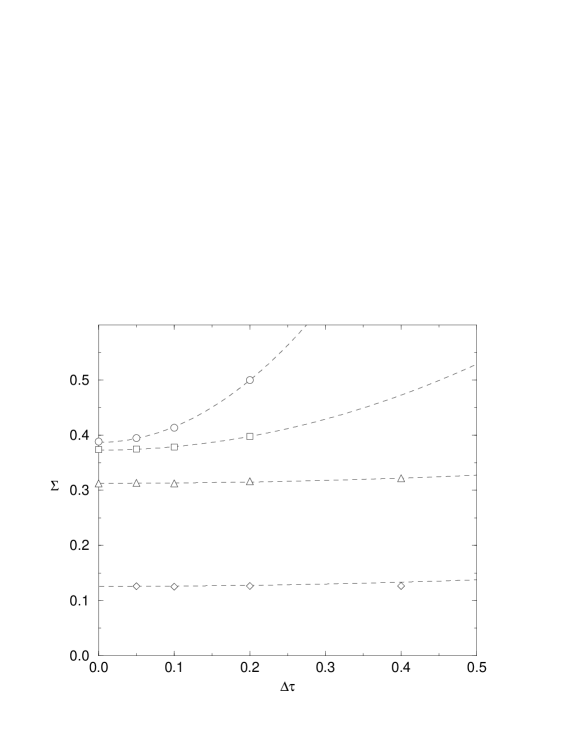
FIG. 1.: The condensate $\Sigma$ plotted against timestep $\Delta\tau$ for $N=0.25$ ($\diamond$), $N=1$ ($\triangle$), $N=3$ ($\sqcap\!\!\!\!\sqcup$) and $N=6$ ($\circ$)

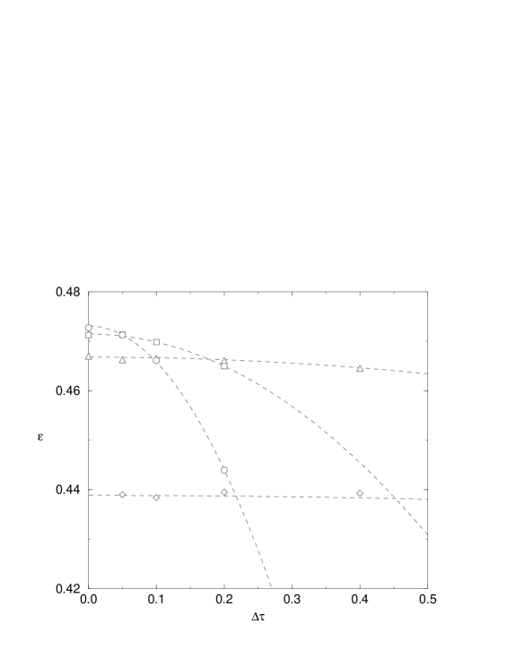
FIG. 2.: Same as Fig. 1 but for the energy density $\epsilon$

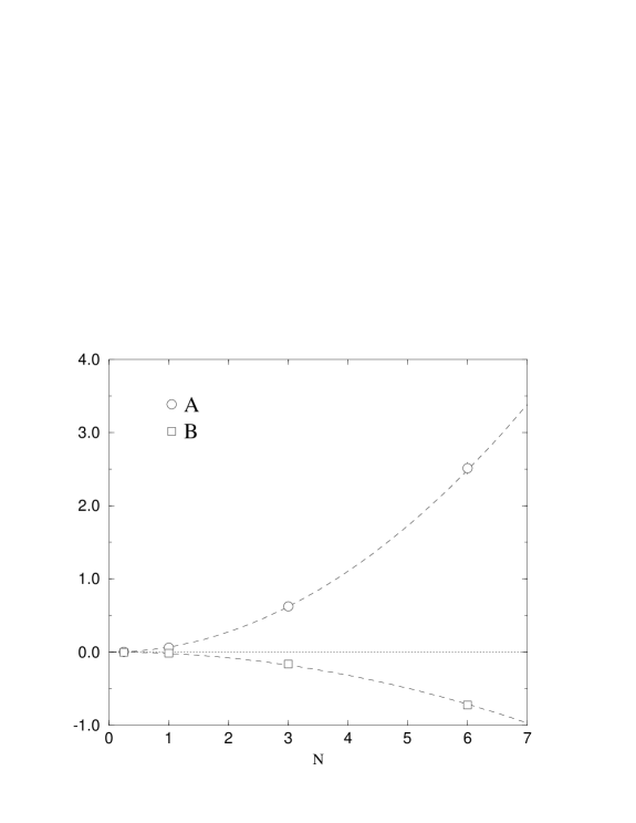
FIG. 3.: Behaviour of the coefficients $A(N)$ and $B(N)$

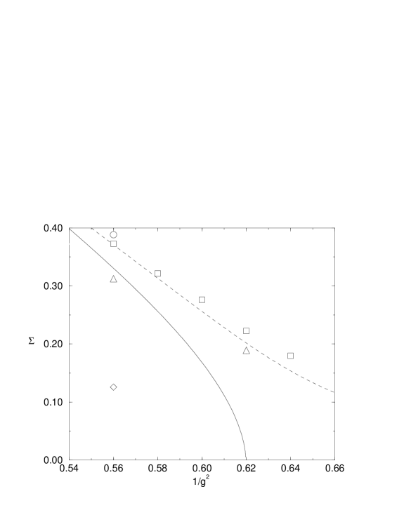
FIG. 4.: Gap equation predictions for $\Sigma$ for $m=0$ (solid line) and $m=0.01$ (dashed line), together with simulation data (see caption to Fig. 1)

FIG. 5.: Fisher plot for fitting form III, $0.52\leq 1/g^{2}\leq 0.55$. The solid lines denote the fitted data.

FIG. 6.: Fisher plot for fitting form II, $0.52\leq 1/g^{2}\leq 0.55$.

FIG. 7.: Fisher plot for fitting form V, $0.52\leq 1/g^{2}\leq 0.55$.

FIG. 8.: Fisher plot for fitting form II, $m\leq 0.01$.

FIG. 9.: Fisher plot for fitting form VI, $m\leq 0.01$.

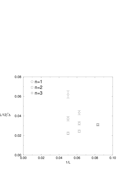
FIG. 10.: $(L/12)^{n}\Delta$ vs. $1/L$ for $1/g^{2}=0.48$.

FIG. 11.: $\Delta$ vs. $1/g^{2}$ for a $16^{4}$ system. The line is a fit to (40).

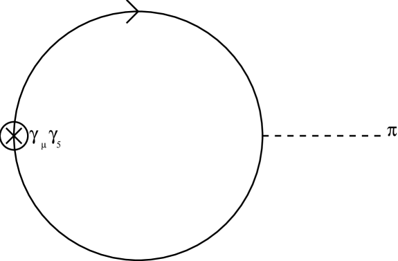
FIG. 12.: Leading order contribution to $f_{\pi}$ in the large-$N_{f}$ approximation.

REFERENCES

- [1] Y. Nambu and G. Jona-Lasinio, Phys. Rev. 122, 345 (1961).
-
[2]
Y. Nambu, in New Trends in Physics,
proceedings of the XI International Symposium on Elementary Particle
Phyics, Kazimierz, Poland, 1988, eds. Z. Adjuk, S. Pokorski and A.
Trautman (World Scientific, Singapore, 1989);
V.A. Miransky, M. Tanabashi and K. Yamawaki, Mod. Phys. Lett. A4, 1043 (1989);
W. Bardeen, C. Hill and M. Lindner, Phys. Rev. D41, 1647 (1990). - [3] B. Rosenstein, B.J. Warr and S.H. Park, Phys. Rev. Lett. 62, 1433 (1989); Phys. Rep. 205, 59 (1991).
- [4] S.J. Hands, A. Kocić and J.B. Kogut, Ann. Phys. 224, 29 (1993).
- [5] A. Hasenfratz, P. Hasenfratz, K. Jansen, J. Kuti and Y. Shen, Nucl. Phys. B365, 79 (1991).
- [6] E. Brézin, J.C. Le Guillou and J. Zinn-Justin, in Phase Transitions and Critical Phenomena vol. 6, eds. C. Domb and M. Green (Academic Press, London, 1976).
- [7] J. Zinn-Justin, Quantum Field Theory and Critical Phenomena, (Oxford Science Publications) (1989).
-
[8]
T. Eguchi, Phys. Rev. D17, 611 (1978);
K.-I. Shizuya, Phys. Rev. D21, 2327 (1980). - [9] A. Kocić and J.B. Kogut, Nucl. Phys. B422, 593 (1994).
- [10] R. Kenna and C. Lang, Nucl. Phys. B393 ,461 (1993).
- [11] M. Göckeler, H.A. Kastrup, T. Neuhaus and F. Zimmermann, Nucl. Phys. B404, 517 (1993).
- [12] S. Kim, A. Kocić and J.B. Kogut, Nucl. Phys. B429, 407 (1994).
- [13] M. Göckeler, R. Horsley, E. Laermann, P.E.L. Rakow, G. Schierholz, R. Sommer and U.-J. Wiese, Nucl. Phys. B334, 527 (1990).
- [14] M. Göckeler, R. Horsley, V. Linke, P.E.L. Rakow, G. Schierholz and H. Stüben, DESY preprint 96-084, hep-lat/9605035 (1996).
- [15] Y. Cohen, S. Elitzur and E. Rabinovici, Nucl. Phys. B220, 102 (1983).
- [16] A. Ali-Khan, M. Göckeler, R. Horsley, P.E.L. Rakow, G. Schierholz and H. Stüben, Phys. Rev. D51, 3751 (1995).
-
[17]
L. Del Debbio and S.J. Hands, Phys. Lett. B373,
171 (1996);
L. Del Debbio, S.J. Hands and J.C. Mehegan, Swansea preprint SWAT/136, hep-lat/9701016 (1997). - [18] S. Duane and J.B. Kogut, Nucl. Phys. B275, 398 (1986).
- [19] S. Gottlieb, W. Liu, D. Toussaint, R.L. Renken and R.L. Sugar, Phys. Rev. D35, 2531 (1987).
- [20] S.J. Hands, S. Kim and J.B. Kogut, Nucl. Phys. B442, 364 (1995).
- [21] H. Kluberg-Stern, A. Morel, O. Napoly and B. Petersson, Nucl. Phys. B220 [FS8], 447 (1983).
- [22] M. Göckeler, private communication.
-
[23]
Th. Jolicœur, Phys. Lett. B171, 143 (1986);
Th. Jolicœur, A. Morel and B. Petersson, Nucl. Phys. B274, 225 (1986). - [24] S. Duane, A.D. Kennedy, B.J. Pendleton and D. Roweth, Phys. Lett. B195, 216 (1987).
-
[25]
A. Kocić, S.J. Hands, J.B. Kogut and E. Dagotto,
Nucl. Phys. B347, 217, (1990);
W.A. Bardeen, S.T. Love and V.A. Miransky, Phys. Rev. D42, 3514 (1990). - [26] P. Hasenfratz and H. Leutwyler, Nucl. Phys. B343, 241 (1990).
- [27] B. Rosenstein and B.J. Warr, Nucl. Phys. B335, 288 (1990).