Abstract

In continuum QCD, nontrivial gauge topologies give rise to zero eigenvalues of the massless Dirac operator. In lattice QCD with Wilson fermions, these zero modes appear as exactly real eigenvalues of the Wilson-Dirac operator and hence as poles in the quark propagator in the vicinity of critical hopping parameter. It is shown that “exceptional configurations,” which arise in the quenched approximation at small quark mass, are the result of the fluctuation of the position of zero mode poles to sub-critical values of hopping parameter on particular gauge configurations. We describe a procedure for correcting these lattice artifacts by first isolating the contribution of zero mode poles to the quark propagator and then shifting the sub-critical poles to the critical point. This procedure defines a modified quenched approximation in which accurate calculations can be carried out for arbitrarily small quark masses.

1 Introduction

The study of QCD in the light quark limit is essential for understanding the chiral structure of pions and implications of the $U(1)$ anomaly which governs the generation of the $\eta^{\prime}$ mass as well as other applications involving the physics of light hadrons. In many previous studies using Wilson-Dirac fermions on the lattice, large statistical errors are encountered in calculations with light quarks and a small subset of the gauge configurations seem to play a dominant role in the final results. These “exceptional configurations” have prevented reliable studies of processes involving very light quarks. Instead, one has been forced to infer the structure of light quark processes from extrapolations based on results obtained for quark masses substantially larger than the physical masses of the up and down quarks. In the quenched approximation, the large fluctuations resulting from exceptional configurations appear to be related to the structure of the small eigenvalues of the Wilson-Dirac operator which can dominate the behavior of the quark propagators [1]. In this paper we show that this behavior is related to a specific artifact of the standard quenched lattice computations. We introduce a modified quenched approximation (MQA) which removes the dominant artifact associated with the Wilson-Dirac formulation of light fermions. With this procedure, the problem of exceptional configurations is removed and the noise associated with light fermion computations is greatly reduced. We also show that the same procedure must be applied to the standard $O(a)$ “improved” actions, such as the Sheikholeslami-Wohlert (Clover) action[2], and could play an important role in improving full unquenched QCD calculations.

In the next section we review the basics of the eigenvalue spectrum of the Wilson-Dirac operator and elucidate the relationship between a pole in a quark propagator at finite mass (sub-critical hopping parameter $\kappa<\kappa_{c}$) and an exceptional gauge configuration. In Section 3 we show how to systematically remove these lattice artifacts. This procedure defines a modified quenched approximation (MQA). This MQA is then contrasted and compared with the unmodifed approach using physical observables in Section 4. In particular, results for the pion mass versus quark mass are presented for both Wilson and Clover actions. The final section contains some general remarks and possibilities for further study.

2 The Eigenvalue Spectrum and Zero Modes

In the quenched approximation, the fermion determinant is removed from the action functional during the Monte Carlo generation of gauge field configurations, so that only the contributions of valence fermions are included. This approximation makes the quenched formulation of the theory particularly sensitive to infrared structure involving light fermions. This sensitivity depends on the particular formulation used to describe fermions in lattice simulations. To understand this sensitivity, it is necessary to explore the structure of the fermion propagators.

The fermion propagator in a background gauge field, $A_{\mu}(x)$, may be written in terms of a sum over the eigenvalues of the Dirac operator,

$${\cal D}f_{i}=\gamma*Df_{i}=\lambda_{i}f_{i}$$ (1)

and

$$S(x,y;\{A\})=\sum_{eigenvalues}\frac{f_{i}(x;A)\bar{g}_{i}(y,A)}{(\lambda_{i}+m_{0})}$$ (2)

where $f_{i}(x,A)$ and $\bar{g}_{i}(x,A)$ are the corresponding eigenfunctions. The mass dependence of the propagator is determined by the nature of the eigenvalue spectrum of the Dirac operator. In the continuum, the euclidean Dirac operator is skewhermitian and its eigenvalues are purely imaginary or zero. Hence, the fermion propagators only have singularities when the real part of the mass parameter vanishes. The behavior of the eigenvalue spectrum near zero determines the nature of dynamical chiral symmetry breaking [3]. The zero eigenvalues, or zero modes, are related to topological fluctuations of the background gauge field by the index theorem associated with the chiral gauge anomaly [4, 5, 6].

The lattice formulation of Wilson-Dirac fermions qualitatively modifies the nature of the eigenvalue spectrum. The Wilson-Dirac operator is usually written as

$${\cal D}\equiv D-rW$$ (3)

$$D_{a\alpha\vec{m},b\beta\vec{n}}=\frac{1}{2}(\gamma_{\mu})_{ab}U_{\alpha\beta}(\vec{m}\mu)\delta_{\vec{n},\vec{m}+\hat{\mu}}-\frac{1}{2}(\gamma_{\mu})_{ab}U^{\dagger}_{\alpha\beta}(\vec{n}\mu)\delta_{\vec{n},\vec{m}-\hat{\mu}}$$ (4)

$$W_{a\alpha\vec{m},b\beta\vec{n}}=\frac{1}{2}\delta_{ab}(U_{\alpha\beta}(\vec{m}\mu)\delta_{\vec{n},\vec{m}+\hat{\mu}}+U^{\dagger}_{\alpha\beta}(\vec{n}\mu)\delta_{\vec{n},\vec{m}-\hat{\mu}})$$ (5)

where $U(\vec{n}\mu)$ are the link matrices associated with the lattice gauge fields, and the parameter $r$ is usually taken to be $1$. The Wilson-Dirac operator is neither skewhermitian (unless $r=0$) nor hermitian. The Wilson term explicitly breaks chiral symmetry and lifts the doubling degeneracy of the pure lattice Dirac action. As a result the eigenvalue spectrum of the Wilson-Dirac operator is no longer purely imaginary but fills a region of the complex plane. The discrete symmetries of the Wilson-Dirac operator imply that the eigenvalues appear in complex conjugate pairs, $(\lambda,{\lambda}^{*})$ and obey reflection symmetries, $(\lambda,-\lambda)$. In addition, there can be precisely real, nondegenerate eigenvalues [7].

Numerical studies of QED in two dimensions [8, 9] and QCD in four dimensions [10, 11], have confirmed the structure of the eigenvalue spectrum as well as the existence of isolated real eigenvalues. In two dimensions, it is possible to study the spectrum of the Wilson-Dirac operator in great detail. The complex eigenvalue spectrum for a typical gauge configuration of QED2 on a $12\times 12$ lattice is shown in Figure 1.

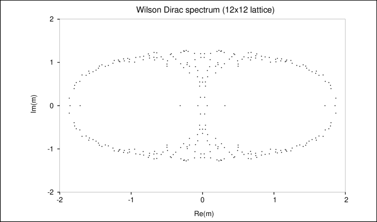
Figure 1: Example of the eigenvalue spectrum for the Wilson-Dirac operator for QED2 on a $12\times 12$ lattice with $\beta=4.5$.

The left, right and central branches of the Wilson-Dirac spectrum are clearly visible, as well as a pair of exactly real eigenvalues for each branch. The left branch is usually associated with the spectrum of the continuum theory and the three other branches correspond to the spectrum of massive doubler modes for QED2; there would be fifteen doubler branches expected for a similar plot of QCD4. The exactly real eigenvalues are the Wilson-Dirac analog of the continuum zero modes. Unlike the situation in the continuum, these real eigenvalues do not all occur at the specific value associated with the zero mass limit, even for real eigenvalues of a given gauge configuration. Because of the fluctuations in the real part of the eigenvalue spectrum, the massless limit can only be defined through an ensemble average in Monte Carlo calculations. We will see that the fluctuations in the position of the zero modes are the primary reason for instabilities in calculations with light Wilson-Dirac fermions [8, 12, 13]. These fluctuations are a direct result of the chiral symmetry breaking which occurs as an artifact of the Wilson-Dirac fermion formulation. Shifts in the positions of the real eigenvalues will cause spurious poles in the fermion propagator for light fermion masses. These nearby poles are the cause of the exceptional configurations encountered in quenched calculations with Wilson-Dirac fermions.

The shifts in the real part of the Wilson-Dirac eigenvalue spectrum are lattice artifacts, as the non-skewhermitian part of the lattice Wilson-Dirac operator is associated with higher dimension operators. In the continuum limit, these artifacts are expected to disappear. In Figure 2, we show the real eigenvalue distribution for our QED2 lattice as a function of $\beta$.

Figure 2: Distribution of real eigenvalues in QED2 near zero fermion mass for $\beta=1.6,2.9,4.5$ and $6.5$ on a $12\times 12$ lattice. Results shown here are for a sample of 1000 independent gauge configurations at each $\beta$. Fermion mass bins were 0.012 wide.

For larger values of $\beta$, the distribution becomes more sharply peaked as expected for the approach to the continuum limit. For any fixed $\beta$, the distribution maintains a finite width and the naive massless limit remains undefined. Indeed the distribution of poles in the corresponding fermion propagators leaves the naive quenched theory formally undefined. For any fixed fermion mass the number of exceptional configurations associated with the zero mode poles can be expected to decrease as $\beta$ is increased, but the limit to infinite Monte Carlo statistics at fixed $\beta$ will not converge[9].

In four dimensions, it is more difficult to study the eigenvalue spectrum, even if we restrict our attention to just the small eigenvalues. The zero modes appear as poles in the fermion propagator

$$(D-rW)f_{i}=\lambda_{i}f_{i}$$ (6)

$$S(x,y;\{U(A)\})_{AB}=\sum_{eigenvalues}\frac{f_{iA}(x;U)\bar{g}_{iB}(y,U)}{\lambda_{i}+1/2\kappa}$$ (7)

$$m_{fermion}=1/2\kappa-1/2\kappa_{c}$$ (8)

where $\kappa$ is the hopping parameter, with the critical value $\kappa_{c}$ determined from the ensemble ensemble average pion mass. For modes with $\lambda_{i}<-1/2{\kappa_{c}}$, the propagator has poles corresponding to positive mass values. The position of these poles can be established by studying any smooth projection of the fermion propagator as a function of $\kappa$. In our computations, we use the integrated pseudoscalar charge to probe for the shifted real eigenvalues

$$Q(\kappa)=\int d^{4}x<\bar{\psi}(x)\gamma_{5}\psi(x)>$$ (9)

We employ the same method that was used by Kuramashi et al.[15] to study hairpin diagrams and the ${\eta}^{\prime}$ mass. A fermion propagator, $G(n,\kappa)$, is computed using a unit source at every site for each color and spin. The result is traced over color and spin and summed over the lattice.

$$Q(\kappa)\rightarrow{\rm Tr}(i\gamma_{5}\sum_{n}G(n,\kappa))$$ (10)

The color averaging over the lattice volume reproduces the integrated charge. This is a global quantity which samples the full lattice volume. By computing its value for a range of kappa values we can search for poles in the fermion propagator. Near a pole, we should find

$$Q(\kappa)\rightarrow\frac{R}{1/\kappa-1/\kappa_{pole}}$$ (11)

In the continuum, the residue R would be directly proportional to the global winding number of the gauge field configuration [8].

In the present calculations we have used eighteen kappa values and a Padé method for fitting the pole structure. This procedure works well if the poles are in the visible region, $\kappa<\kappa_{max}<\kappa_{c}$. Although we had originally hoped to determine the complete spectrum of real eigenvalues using this method, it was only found to be reliable if the poles were in the “visible” region. There we could determine the pole positions and the relevant eigenvalues to great precision. An example of these scans is shown in Figure 3 for Wilson fermions.

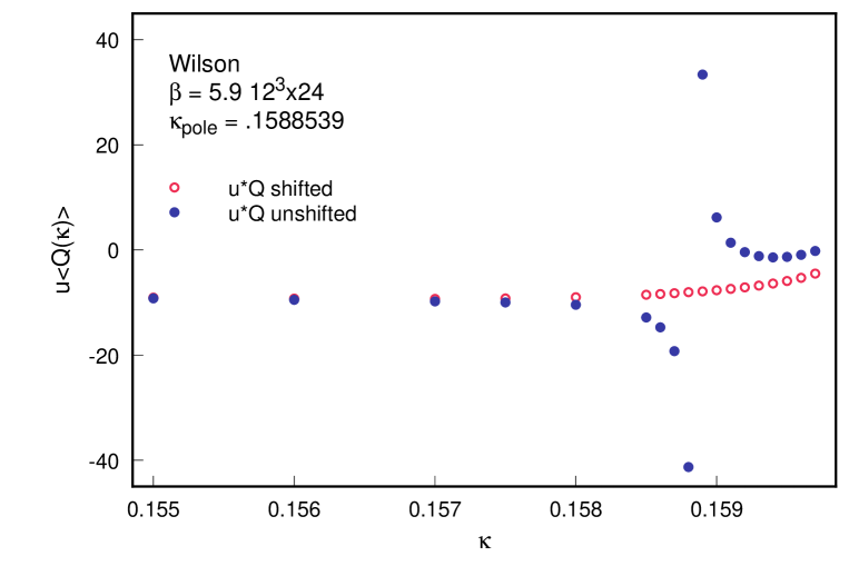
Figure 3: $uQ(\kappa)$ is shown as a function of kappa for Wilson action configuration 114000. Here $u$ is twice the bare quark mass and $Q(\kappa)$ is the (space-time) average pseudoscalar charge density. The unshifted charge (denoted by solid dots) has a pole at $\kappa=.1588539$. In contrast the charge in the modified quenched approximation (denoted by open cirles) shows only smooth behaviour.

The existence of isolated poles is obvious from this figure. The value of the integrated pseudoscalar charge can be computed, with no appreciable slowdown in convergence, for values of the hopping parameter arbitrarily close to the pole position.

For the computations in this paper, we use a sample of 50 gauge configurations available from the ACPMAPS library, the e-lattice set [17]. These configurations were generated on a $12^{3}\times 24$ lattice at $\beta=5.9$ and are separated by 2000 sweeps. We determine pole eigenvalues for both the standard Wilson-Dirac action and a Clover action with a clover coefficient of $C_{SW}=1.91$ corresponding to the value suggested by Lüscher [18]. We find six configurations with visible poles for each choice of fermion action. These results are shown in Table I. It is important to note that only one gauge configuration is in common between the two sets of visible poles. This emphasizes the point that the existence of visible poles for a particular gauge configuration is a sensitive artifact of the particular choice of fermion action. As the fermion action is varied, the real eigenvalues move, some to smaller values of kappa where they may become visible and some to larger values of kappa where they may not be observed as visible poles. Therefore, the visible poles, and the corresponding identification of exceptional configurations is a sensitive property of the fermion action and not a property unique to the particular gauge configuration. In the same vein, a small change in the clover coefficient may remove a visible pole for one configuration and add a visible pole for another configuration, completely changing identification of the exceptional configurations. Since only a collision of two real modes allows the pairing required to move off the real axis, small changes in the parameters of the fermion action should not change the number of isolated real modes but only their visibility.

Table 1: Visible poles for a set of 50 gauge configurations (102000-200000 step 2000).

Wilson Action			Clover Action, CSW = 1. 91
Conf.	$\kappa_{pole}$	PS residue	Conf.	$\kappa_{pole}$	PS residue
114000	0.1588539	-2.1463	122000	0.1331519	+3.3366
132000	0.1594870	-2.4800	150000	0.1339044	+4.8900
148000	0.1593216	-3.6325	160000	0.1334519	-2.0718
160000	0.1593803	-2.8494	162000	0.1335898	-2.5609
182000	0.1593803	+2.5036	178000	0.1334681	-23.4917
194000	0.1595557	-5.3055	178000	0.1337479	+22.7462
			198000	0.1337620	+1.5828

The connection between the visible poles and the exceptional configurations is made clear if we plot the time dependence of a pseudoscalar meson propagator for a kappa value associated with a light quark, e.g. $\kappa=0.1595$. In Figure 4, we plot all fifty configurations where the configurations

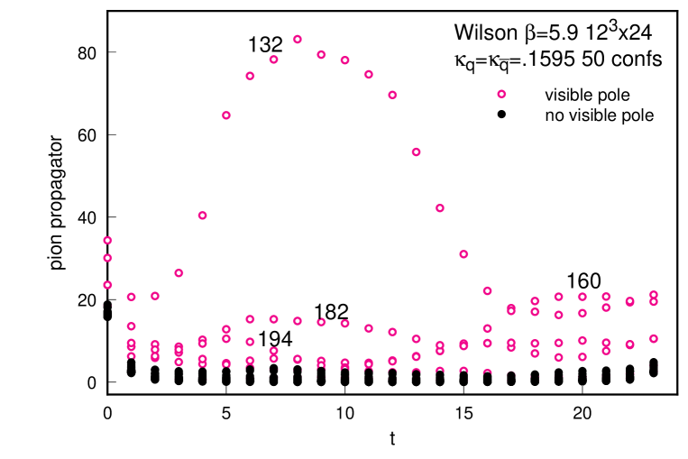
Figure 4: Pion propagator for $\kappa=.1595$ showing all 50 configurations. Propagators for configurations with visible poles are displayed with open circles and labeled by their sequence number when appropriate.

with visible poles have been labeled with open circles. It is clear, that all of the distorted propagators associated with the exceptional configurations can be uniquely identified with the presence of nearby visible poles.

3 The Modified Quenched Approximation

In the standard quenched approximation, only the valence fermion contributions are calculated explicitly from the fermion propagators and the effects of the fermion loop determinant are ignored. This approximation is very sensitive to singularities of the fermion propagator which may be encountered in particular formulations of lattice fermions. In this section, we identify those singularities which are due to artifacts of Wilson-Dirac fermions in quenched lattice calculations. We give a simple prescription which corrects for the principal artifacts encountered when using the Wilson-Dirac fermion formulation for light quark masses.

As noted in the previous section, the eigenvalue spectrum of Wilson-Dirac fermions generally contains a number of isolated real eigenvalues. In the continuum limit, these eigenvalues are identified as zero modes and occur at precisely zero fermion mass. In the Wilson-Dirac formulation, these eigenvalues shift due to the chiral symmetry breaking generated by the Wilson-Dirac action. Some of these eigenvalues are shifted to positive mass which causes singular behavior for the fermion propagators computed for a mass near a shifted eigenvalue. Because of these shifts, there is no common critical value of the fermion mass or hopping parameter, even for a specific gauge configuration. The critical value of the hopping parameter is normally defined by the chiral limit as determined by the ensemble average of the pseudoscalar meson mass over all configurations. In general, these eigenvalue shifts would be averaged to zero in the ensemble average and no specific corrections would be needed. However, in the quenched approximation, the shifts cause poles in the fermion propagators which are not properly averaged. This effect corresponds to similar situations in degenerate perturbation theory where small perturbative shifts can cause large effects due to small energy denominators. In this case it is known that it is essential to expand around the exact eigenvalues and compensate the perturbation expansion with counter-terms in each order. In the present case, we argue that a similar compensation must be made when using Wilson-Dirac fermions. Fortunately, we know that the correct position for the real poles is a common critical value of the hopping parameter, $\kappa_{c}$ associated with the massless fermion limit.

We are now able to devise a procedure for correcting the fermion propagators for the artifact of the visible shifted poles. As before, we write the fermion propagator as a sum over the eigenvalues of the Wilson-Dirac operator,

$$S(x,y;\{U(A)\})_{AB}=\sum_{eigenvalues}\frac{f_{iA}(x;U)\bar{g}_{iB}(y,U)}{\lambda_{i}+1/2\kappa}$$ (12)

The shifted real eigenvalues cause poles at particular values of the hopping parameter. The residue of the visible poles can be determined by computing the propagator for a range of kappa values close to the pole position and extracting the residue for the full propagator. It is convenient to have first determined the pole position very accurately from a global quantity such as the integrated pseudoscalar charge before extracting the propagator residue. With this residue we can define a modified quenched approximation by shifting the visible poles to $\kappa=\kappa_{c}$ and adding terms to compensate for this shift when the hopping parameter is not near the position of the visible poles. We are able to apply this procedure because it removes a specific lattice artifact, and we know the correct continuum position of all real eigenvalues.

As an example we can apply this procedure to the integrated pseudoscalar charge. In Equation (11) we determined the visible pole position and residue by studying the $\kappa$ dependence of $Q(\kappa)$. Once this has been determined we could define a modified quenched approximation by moving the visible pole to kappa critical. The naive result would be

$$Q(\kappa)\rightarrow Q(\kappa)-\frac{R}{(1/\kappa-1/{\kappa_{pole}})}+\frac{R}{(1/\kappa-1/{\kappa_{c}})}$$ (13)

The impact of this modification is shown in Figure 3 for Wilson-Dirac fermions. The same behaviour is observed in the case of the SW improved Clover action. The shift removes the spurious pole and allows a smooth extrapolation to zero fermion mass, $\kappa\rightarrow\kappa_{c}$.

The above procedure corrects for the leading effects but may distort an ensemble average by only shifting visible poles and not compensating for poles beyond the visible range. Therefore we chose to define the modified quenched approximation (MQA) using a compensated shift of the visible poles which moves the visible poles while preserving the ensemble averages at large mass. Introducing a mass parameter, u, relative to a common critical value of the hopping parameter, $\kappa_{c}$,

$$u=1/\kappa-1/{\kappa_{c}}=2{m_{f}}a$$ (14)

the visible pole may be replaced as follows

$$\frac{1}{u-u_{pole}}\rightarrow\frac{2}{u}-\frac{1}{(u+u_{pole})}$$ (15)

At large mass the first two terms in the expansion in $1/u$ are not modified and terms linear in the shifts should average to zero. Since we are only able to identify poles with positive mass shifts, we have compensated a visible pole with one shifted to negative mass. These negative shifts do not generate singularities in the fermion propagators computed for positive mass values and are expected to cancel against poles with negative shifts generated by other configurations in the ensemble. With this procedure, we do not expect any large renormalization of $\kappa_{c}$ due to the shifting procedure.

The full MQA fermion propagator may be simply computed by adding a term to the naive fermion propagator which incorporates a compensated shift of the visible poles. The modified propagator is given by

$$S^{MQA}(x,y;\{U(A)\})\equiv S(x,y;\{U(A)\})+a_{pole}(\kappa)*{\rm res}_{pole}(x,y)$$ (16)

where

$$a_{pole}(\kappa)\equiv-\frac{1}{u-u_{pole}}+\frac{2}{u}-\frac{1}{(u+u_{pole})}$$ (17)

and

$${\rm res}_{pole}(x,y)\equiv f_{pole}(x,U)\bar{g}_{pole}(y,U)=\lim_{u\rightarrow u_{pole}}(u-u_{pole})*S(x,y,\{U\})$$ (18)

As noted above, the propagator residue can be determined by computing the fermion propagator at values arbitrarily close to the pole position. The residue of each pole is extracted by calculating the propagator at $u_{pole}-\Delta$ and $u_{pole}+\Delta$ with $\Delta\approx 10^{-5}$ where the pole position, $u_{pole}$, has been accurately determined from the integrated pseudoscalar charge measurement. These calculations generate only a modest overhead for the computations as only the configurations with visible poles need to be corrected. For our sample at $\beta=5.9$ ($12^{3}\times 24$), about 10 to 15% of the configurations need to be corrected for visible poles. At larger physical volumes for fixed $\beta$, a larger percentage of configurations should be affected; while at higher $\beta$ for fixed physical volume, a smaller percentage of configurations should be affected.

The MQA propagator may now be used to evaluate any correlation functions involving Wilson-Dirac fermions. We have simply removed an obvious lattice artifact from the fermion propagator which distorts the usual quenched approximation. It is important to note that the artifact is the appearance of visible poles at positive mass, not the existence of small or real eigenvalues. It is only the visibility that we have corrected by appealing to the correct behavior in the continuum limit. We proceed to discuss some applications of the Modified Quenched Approximation in the next section.

4 Applications

The MQA quark propagators defined in the previous section may be used in place of the usual quenched propagators to compute any hadron physics properties accessible in the quenched approximation. We expect that the suppression of the large fluctuations normally associated with the exceptional configurations should greatly reduce the errors associated with the propagation of light quarks. The most sensitive quantities are those associated with the chiral limit. Prime examples are the pion propagator, the hairpin calculation for the $\eta^{\prime}$ mass, meson decay constants and the light hadron spectrum.

We illustrate the impact of the Modified Quenched Approximation by computing the pseudoscalar propagator for a range of quark masses including values appropriate to physical light quarks. As mentioned in Section 2, we use a sample of 50 gauge configurations generated on a $12^{3}\times 24$ lattice at $\beta=5.9$, the ACPMAPS e-lattice set [17]. We computed the two-point pion correlation function, $G_{\pi\pi}(t)$, for smeared source and sink using an approximation to the pion wavefunction in Coulomb gauge. In Figure 5, we show the time dependence of the resulting pion propagators using the usual quark propagators obtained for the Wilson-Dirac action for a range of hopping parameter values.

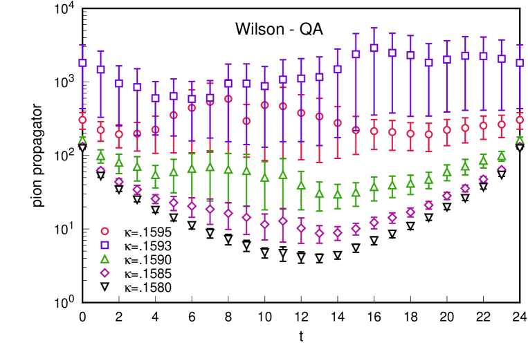
Figure 5: Pion propagators versus lattice time for Wilson action with naive quark propagators at $\kappa=.1580,.1585,.1590,.1593$ and $.1595$. $m_{q}=m_{\overline{q}}$.

The errors shown are highly correlated. For the larger values of the hopping parameter, corresponding to the lighter quark masses, the large fluctuations do not permit a sensible fit to a pion propagator. In Figure 6, we show the same plot where the quark propagators have been replaced by the MQA propagators.

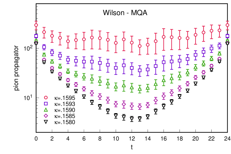
Figure 6: Pion propagators versus lattice time for Wilson action with MQA quark propagators at $\kappa=.1580,.1585,.1590,.1593$ and $.1595$. $m_{q}=m_{\overline{q}}$.

Of the 50 configurations, six were found to have visible poles with the pole positions as given in Table I. The MQA propagators were computed using the procedures of Section 3 with $\kappa_{c}=0.15972$. We find the fluctuations are greatly suppressed allowing a measurement of the pion mass even for the largest hopping parameter value. (This value of kappa corresponds to a light quark mass not much larger than the average physical up and down masses.) Even for heavier masses, the errors appear to be greatly reduced by using the MQA propagators.

The same analysis has been applied to the case of fermions defined through the improved Clover action. Again we find that there are large fluctuations for the hopping parameter values corresponding to the light quark limit. The pion propagators computed using the MQA quark propagators show greatly reduced fluctuations. In Table I, there are six configurations with visible poles for the Clover action although one configuration exhibits two visible poles. Only one gauge configuration has visible poles for both Wilson-Dirac and Clover actions. Again, the MQA analysis is seen to greatly reduce the fluctuations of the pion propagator. Here we have used $\kappa_{c}=0.13425$ for the critical hopping parameter. It is clear that clover improvement does not mitigate the problem of visible poles although the MQA analysis is equally effective for the Wilson-Dirac and Clover actions.

The pion propagators we have shown are computed with the limited statistics of 50 gauge configurations. For the lighter quark masses, it is clear that the normal analysis would not be limited by statistics but by the frequency of exceptional configurations associated with visible poles. However, we believe that the MQA analysis cures this problem and higher statistics would now greatly improve the accuracy of computations with light mass quarks. We can isolate the effect of the real pole by extracting its residue from a fit to a series of pion propagators in which only one quark mass is varied. The results of that procedure for a particular configuration (148000) with a pole in the visible region is shown in Figure 7.

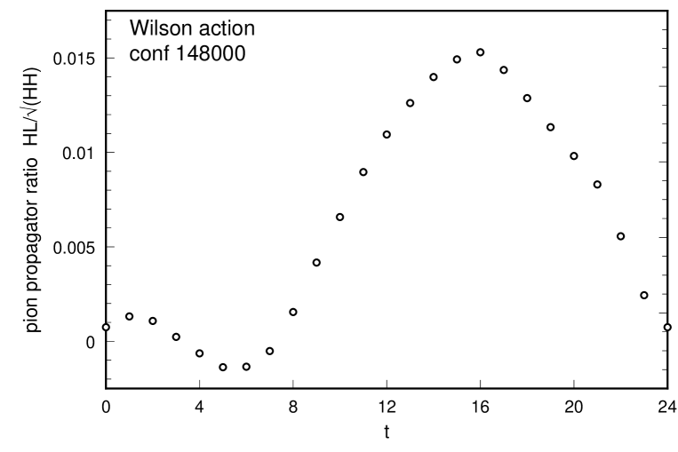
Figure 7: Real mode pole residue at $\kappa=.1593216$ for configuration 148000 with Wilson action. The residue is computed using the ratio of heavy-light pion propagator normalized by the square root of the heavy-heavy propagator. Here the heavy quark is $\kappa=.1570$ and the light quarks used have $\kappa=.1595{\rm-}.1590$.

Another way to see the effects of using the MQA analysis employs a bootstrap procedure. We create 200 bootstrap sets of 50 configurations each randomly selected from the full set of 50 gauge configurations. We simultaneously fit the three pion two-point correlators LS(local-smeared), SL(smeared-local) and SS(smeared-smeared) to a common pion mass. Each correlator has the form:

$$G_{\pi\pi}(t)=|A|^{2}2\cosh(m_{\pi}t)$$ (19)

We determine fits to the pion mass, $m_{\pi}$, and coupling amplitudes, $|A_{L}|$ and $|A_{S}|$, for each of the 200 bootstrap sets for particular values of the hopping parameter. In Figure 8, scatter plots compare the fluctuations and correlations for Wilson-Dirac fermions before and after using the MQA analysis.

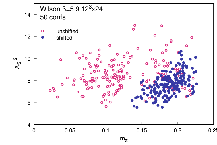
Figure 8: Pion mass, $m_{\pi}$, and coupling amplitude, $|A_{S}|$, extracted from the pseudoscalar-pseudoscalar correlator using smeared source and sink operators. The results for 200 bootstrap samples are displayed with naive (open circles) and MQA shifted (solid dots) Wilson action quark propagators.

It is clear that the MQA analysis greatly reduces the fluctuations and produces a more tightly correlated fit for the mass and decay constant. Again, we would expect even more dramatic improvement with a larger statistics sample of gauge configurations.

Using the full bootstrap set, we have made an uncorrelated fit for the pion mass and decay constants where the quark masses range over all eight values of the hopping parameter considered in this paper. We use data on correlation functions for smeared and local pseudoscalar sources and the local axial vector charge density for our analysis. In Figure 9, we plot the square of the measured values of the pion mass for Wilson-Dirac fermions against the average of the quark masses, $m_{l}\equiv(m_{q1}+m_{q2})/2=(0.5/k_{q1}+0.5/k_{q2}-1/\kappa_{c})/(2a)$, for the naive and MQA analysis, respectively.

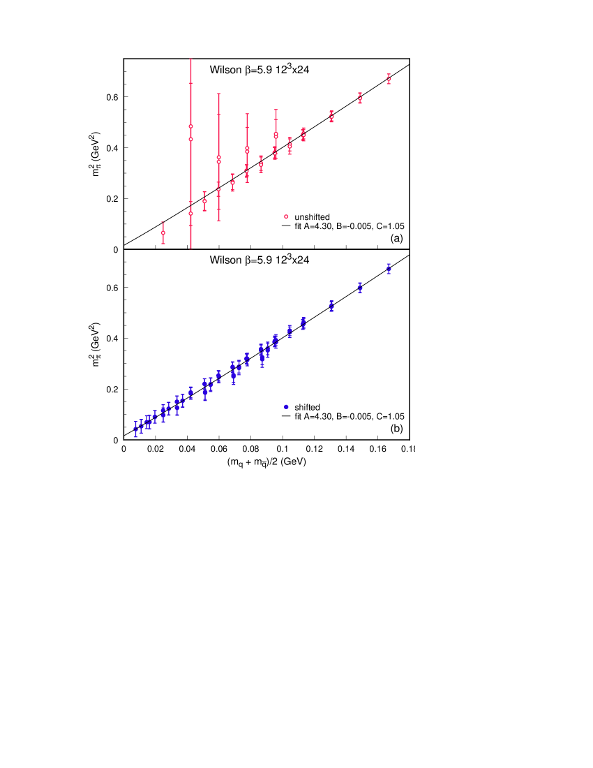
Figure 9: Pion mass plots for Wilson action with (a) naive quark propagators in the kappa range, kappa = 0.1550 to 0.1590 (open circles) and (b) MQA propagators in the full kappa range, kappa = 0.1550 to 0.1595 (dots). A power law fit (Eq. 20) to the MQA masses is also shown.

The large fluctuations in the naive analysis come when one or both of the quarks are light. We show a simple best fit for the pion mass squared as a function of the average bare quark masses, $m_{l}$, assuming the general power law form:

$$m_{\pi}^{2}=A(m_{l}-B)^{C}$$ (20)

The masses determined from the MQA analysis seem to give a good fit to a nearly linear behavior with little evidence for a modified power law (C=1.05). The slope determined by our fit is $m_{\pi}^{2}/m_{l}=4.30$ which is in good agreement with previous measurements [17]. The fit also yields a new critical value for the hopping parameter, $\kappa_{c}=0.159725$, which should be compared with the value of $\kappa_{c}=0.15972$ obtained from the standard analysis. The small shift in $\kappa_{c}$ reflects our use of a compensated shift for the visible poles and the linearity observed in our mass fits. If uncompensated shifts were used for the visible poles, or if the value of the critical hopping parameter were varied slightly, a modest renormalization of $\kappa_{c}$ would be expected for the MQA analysis compared to the normal procedure. In extreme cases, it may be necessary to iterate the shift process to determine a consistent value of $\kappa_{c}$.

We also show plots of the fits for the Clover action with and without MQA analysis in Figure 10.

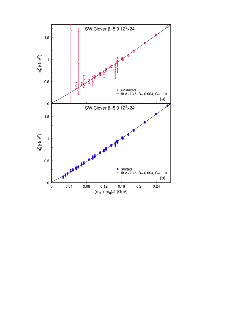
Figure 10: Pion mass plots for SW Clover action with (a) naive quark propagators in the kappa range, kappa = 0.1290 to 0.1335 (open circles) and (b) MQA propagators in the full kappa range, kappa = 0.1290 to 0.1337 (dots). A power law fit (Eq. 20) to the MQA masses is also shown.

Of course, the slope $m_{\pi}^{2}/m_{l}$ here will differ significantly from the previous case (using naive Wilson action at $\beta=5.9$). Using the clover coefficient $C_{SW}=1.91$, we find $m_{\pi}^{2}/m_{q}=7.45$. Otherwise, the general conclusions are the same in the Clover case as in the Wilson case.

Another quantity with considerable infrared sensitivity is the hairpin contribution to the singlet pseudoscalar mass term which is thought to be responsible for the large $\eta^{\prime}$ meson mass in quenched QCD. We follow the analysis of Kuramashi et al. [15] and use the all-source propagators discussed previously in computing the pseudoscalar densities. The hairpin contribution to the $\eta^{\prime}$ propagator can be isolated using appropriate color projections of the two point correlation function of the all-source propagators[16]. As in the case of the pion propagator, the large fluctations observed for lighter quark masses in the naive analysis are sharply reduced by the MQA analysis. A detailed study of the hairpin propagator with high statistics is underway and results will be presented elsewhere.

In this paper, with our low statistics, we restrict our attention to the pseudoscalar charge squared, $Q(\kappa)^{2}$. The weighted average of the square of this charge, $<(u^{*}Q(\kappa))^{2}>$, as $\kappa$ approaches $\kappa_{c}$ is the average of square of the winding number and therefore a measure of the topological susceptibility of QCD. In Figure 11, we show our results for the $<(u^{*}Q(\kappa))^{2}>$ as a function of kappa the MQA analysis as well as for the naive analysis (with and without exceptional configurations excluded).

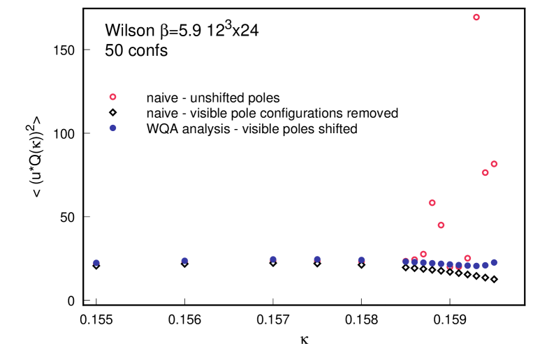
Figure 11: $<(u^{*}Q(\kappa)^{2}>$ as a function of kappa for Wilson action. Results are shown for the MQA analysis as well as the naive analysis (with and without exceptional configurations).

As shown in Figure 11, the results for naive quenched analysis including all configurations is not even smooth as $\kappa\rightarrow\kappa_{c}$. The full MQA analysis produces a smooth and nearly flat result. If we had simply excluded the expectional configurations the result is smooth but differs in detail from the MQA analysis. In particular, the value of $\kappa_{c}$ needed to obtain flat behaviour is shifted.

5 Discussion and Conclusions

We have seen that the Wilson-Dirac operator has exact real modes in its eigenvalue spectrum. In the quenched approximation, these real modes can generate unphysical poles in the valence quark propagators for physical values of the quark mass. These poles can produce large lattice artifacts and are the source of the exceptional configurations observed in attempts to directly study QCD in the light quark limit. Indeed, we have observed poles corresponding to quark masses as large as 20-30 MeV which is much larger that the physical light quark masses.

We have shown that a simple procedure can be devised to completely remove this artifact in realistic calculations. The Modified Quenched Approximation identifies and replaces the visible poles in the quark propagator by the proper zero mode contribution, compensated to preserve the proper ensemble averages at large mass. The MQA propagator can then be used to compute all physical quantities normally accessible in the quenched approximation. Since only a small number of configurations require modification (10% for our lattice at $\beta=5.9$), there is only a modest overhead cost required to apply the full MQA analysis. As presented here, the only potentially time-consuming part of using the MQA analysis is the initial identification of the configurations which have visible poles. In this paper, we used a scan involving the integrated pseudoscalar charge and 18 $\kappa$ values to determine the visible pole positions. Subsequently, we have also found that inverting only one color-spin component of the all source quark propagator and using 12 reasonably spaced $\kappa$ values near $\kappa_{c}$ works well and the computational cost is quite modest. For larger values of $\beta$, a smaller number of configurations should be affected at fixed physical volume.

The MQA analysis allows stable quenched calculations with very light quark masses and reduces the errors even in the case of heavier quark mass. In the normal analysis, the presence of exceptional configurations limits the usefulness of large statistical samples in many problems. The number of exceptional configurations simply grows with the statistical sample. With the MQA analysis the exceptional configurations are eliminated and the errors can be meaningfully reduced by using larger statistical samples.

We have examined both Wilson-Dirac and the improved Clover actions. The Clover action is designed to remove O(a) lattice artifacts in the Wilson action. However, we have found that this form of improvement does not remove the problem of visible poles and exceptional configurations. Indeed, we seem to find the same size spread of the real eigenvalues for both Wilson-Dirac and Clover actions. A similar conclusion concerning the frequency of exceptional configurations was reached in a different context by Lüscher [18].

In some applications, the use of improved actions has been combined with coarse lattices to avoid the large numerical overhead associated with very fine grained simulations. The MQA analysis may be an essential ingredient in realistic applications of these methods.

The complete unquenched theory does not suffer explicitly from singularities associated with the problem of shifted poles. The fermion determinant is formally the product of the eigenvalues of the Wilson-Dirac operator, $(\lambda_{i}+1/2\kappa)$. When multiplied by the fermion determinant, all of the poles in the sum of the valence fermion propagators and hairpin terms are canceled. There are now no singularities associated with the real eigenvalues and their shifts are simply averaged when summed over the ensemble of configurations. For this cancellation to occur, it is essential that the zeros of the fermion determinant match exactly the poles of the fermion propagators and hairpin contributions. Without this precise cancellation, the shifted real eigenvalues still introduce singular terms. For example, if the mass used in the fermion determinant is not exactly the same as the mass used in the propagators, the cancellation fails. Hence, it may still be necessary to use the MQA analysis in conjunction with an approximate evaluation of the fermion determinant in realistic unquenched simulations. In this case, the sensitive poles are shifted to a common mass value and the remaining averages involve insensitive contributions or terms which have been effectively moved to the numerator. Here it is essential to realize that the shifted real eigenvalues are artifacts of the specific lattice fermion action employed in the calculation and are not to be associated with real physical effects of the unquenched theory.

The complex eigenvalues of the Wilson-Dirac action are also affected by shifts in the real part of the eigenvalues as is clear from the way the doubler states are removed from the physical spectrum. Contributions associated with eigenvalues with small imaginary parts may also be sensitive to shifts in the real part. However, artifacts associated with these shifts may be suppressed by finite volume effects in realistic simulations where there are very few eigenvalues with small imaginary parts except for the purely real eigenvalues we have previously discussed. In the infinite volume limit, it may be necessary to re-examine the precise structure of all small eigenvalues of the Wilson-Dirac action. We suggest that the MQA method should suffice to remove the singular terms encountered in realistic calculations using Wilson-Dirac fermions or similar improved actions. We have not examined other formulations of lattice fermions, such as Kogut-Susskind fermions, which do not suffer directly from lattice artifacts associated with the real eigenvalue spectrum.

6 Acknowledgements

The computations were performed on the ACPMAPS at Fermilab. The work of W.B., E.E, and G.H. was performed at the Fermi National Accelerator Laboratory, which is operated by Universities Research Association, Inc., under contract DE-AC02-76CHO3000. The work of A.D. was supported in part by NSF grant 93-22114. The work of H.T. was supported in part by the Department of Energy under grant DE-AS05-89ER 40518.

References

- [1] K.-H. Mutter, Ph. De Forcrand, K. Schilling and R. Somer, in Brookhaven 1986, Proceedings, Lattice Gauge Theory, ’86, pg. 257.
- [2] B.-Sheikholeslami and R. Wohlert, Nucl. Phys. B259 (1985) 572; G. Heatlie, G. Martinelli, C. Pittori, G. C. Rossi and C. T. Sachrajda, Nucl. Phys. B352 (1992) 266.
- [3] T. Banks and A. Casher, Nucl. Phys. B171 (1980) 103.
- [4] G. ‘t Hooft, Phys.Rev.Lett.37, (1976)8.
- [5] M. Atiyah and I. Singer, Ann. of Math. 87 (1968) 485; M. Atiyah and G. Segal, Ann. of Math. 87 (1968) 531; M. Atiyah and I. Singer, Ann. of Math. 97 (1972) 119, 139.
- [6] H. Leutwyler and S. Smilga, Phys. Rev. D 46, (1992) 5607.
- [7] J. Smit and J. Vink, Nucl. Phys. B286 (1987)485.
- [8] J. Smit and J. Vink, Nucl. Phys. B284 (1987) 234; J. Vink, Nucl. Phys. B307 (1988) 549.
- [9] W. Bardeen, A. Duncan, E. Eichten and H. Thacker, Fermilab-PUB-97/119-T.
- [10] R. Setoodeh, C.T.H. Davies and L.M. Barbour, Phys. Lett. B213 (1988)195. L. M. Barbour et al., Phys. Rev. D 46 (1992) 3618.
- [11] J.J.M Verbaarschot, hep-lat/96-06009
- [12] Y. Iwasaki, Nucl. Phys. B (Proc. Suppl.) 9 (1989)254.
- [13] S. Itoh, Y. Iwasaki and T. Yoshie, Phys. Lett. B184 (1987)375; S. Itoh, Y. Iwasaki and T. Yoshie, Phys. Rev. D 36 (1987) 527.
- [14] Ph. De Forcrand, R. Gupta, S. Gusken, K.-H. Mutter, A. Patel, K. Schilling and R. Sommer, Phys. Lett. B200 (1988) 143.
- [15] Y. Kuramashi, M. Fukugita, H. Mino, M. Okawa and A. Ukawa, Phys. Rev. Lett. 72 (1994)3448.
- [16] A. Duncan, E. Eichten, S. Perrucci and H. Thacker, hep-lat/96-08110.
- [17] A. Duncan, E. Eichten, J. Flynn, B. Hill, G. Hockney and H. Thacker, Phys. Rev D 51 (1995) 5101.
- [18] M. Luscher, S. Sint, R. Sommer, P. Weisz and U. Wolff, hep-lat/96-09035.