Abstract

We examine the lattice boundary formulation of chiral fermions with either an explicit Majorana mass or a Higgs-Majorana coupling introduced on one of the boundaries. We demonstrate that the low-lying spectrum of the models with an explicit Majorana mass of the order of an inverse lattice spacing is chiral at tree level. Within a mean-field approximation we show that the systems with a strong Higgs-Majorana coupling have a symmetric phase, in which a Majorana mass of the order of an inverse lattice spacing is generated without spontaneous breaking of the gauge symmetry. We argue, however, that the models within such a phase have a chiral spectrum only in terms of the fermions that are singlets under the gauge group. The application of such systems to nonperturbative formulations of supersymmetric and chiral gauge theories is briefly discussed.

1 Introduction

On a lattice left-handed Weyl fermions $\psi$ are always accompanied by their right-handed counterparts $\chi$, unless certain mild conditions for the action are broken [1]. Such a doubling is present both in the Wilson [2] and in the domain wall formulations [3, 4] (for a review, see [5]), being the main obstacle to the non-perturbative definition of chiral gauge theories. So far all attempts to make the chiral counterpart $\chi$ sterile, in a way that does not use a hard breaking of gauge symmetry and leaves an interacting chiral theory, have failed (see, for example, reviews [8, 5, 9] and references therein).

Another conceivable way to define a theory with only fermion fields $\psi$ is to decouple $\chi$ by giving them Majorana masses of the order of the inverse lattice spacing. It can be done directly if the fermions belongs to real representation of the gauge group. If they belong to complex representation, a generalized Higgs mechanism is to be employed in order the Majorana mass not to break the gauge invariance. In this case model must have strong coupling paramagnetic (PMS) phase, where fermions acquire masses of the order of the inverse lattice spacing, while the gauge symmetry is not spontaneously broken, i.e. no chiral condensate or no vacuum expectation value of the Higgs fields arise (for a review and further references, see [10]).

In the Wilson formulation, the $\psi$ and $\chi$ are coupled through the Wilson term. Therefore the introduction of a Majorana mass for $\chi$ generates a Majorana coupling for $\psi$. So in the gauge theory fine tuning becomes necessary not only for Dirac mass but also for Majorana mass of $\psi$. Furthermore, in the case of complex representations, there arises a serious problem with the properties of the model within the PMS phase, where its spectrum either becomes vectorlike, or consists only of neutral, i.e. singlet under the gauge group, chiral fermions, whose gauge interactions very likely vanish in the continuum limit [11, 12, 13, 14]. In the domain wall formulation the chiral fermions $\psi$ and $\chi$ appear as collective states of coupled five-dimension fermions. These states are localized at two surfaces formed by mass defects in the five-dimensional system [3] or by free boundaries of the five-dimensional space [4]. These surfaces are separated in the fifth dimension and the overlap between these states is suppressed exponentially with this distance. This gives rise to a hope that the above problems can be avoided in such a formulation.

This, in fact, is underlying idea of the recent proposal [15] for lattice formulation of the Standard Model. In order to generate the Majorana mass for the collective state $\chi$, it has been suggested to introduce on the surface at which $\chi$ is localized certain gauge invariant four-fermion interactions motivated by the approach [16]. A similar idea is followed by the proposal [17] for lattice formulation of $N=1$ supersymmetric theories. In this case the Majorana mass is introduced on the same surface directly, for the fermions belong to real representation.

Thus, yet more questions, which should be answered first, arise in such an approach: ($i$) Whether the generation of the Majorana mass on one of the surfaces leads to the chiral spectrum of the model? This question is common to both proposals, [15] and [17], and requires special investigation, since the chiral states in the domain wall formulation do not present in the action explicitly. ($ii$) Whether the PMS phase exists in the systems employing the Higgs mechanism? Although some indirect arguments in favour of the presence of the PMS phase has already been given in [15], it seems interesting to look at the problem from a more general point of view. ($iii$) Does the model has chiral spectrum in the PMS phase, and if so, what fermions, charged or neutral, form it? This is a crucial question to all formulations of chiral gauge theories that employ the PMS phase.

The aim of this paper is to answer these questions. We consider the variant of the domain wall formulation with free lattice boundaries [4] and the Majorana mass or Higgs-Majorana coupling introduced on one of the boundaries. These models are introduced in Section 2. In Section 3 we analyze the fermion propagators in the model with the Majorana mass and gauge fields switched off, and show that the low-lying spectrum of such a model is chiral. In Section 4 using a mean-field technique we demonstrate the existence of the PMS phase in the systems with the Higgs-Majorana coupling. In Section 5 we consider such systems within the PMS phase and argue that they may have chiral spectrum only for the fermions that are singlets under the gauge group. Section 6 contains a summary and a discussion of possible applications of such models.

Our conventions are the following. We consider Euclidean hypercubic $5$-dimensional lattice with spacing $a$, which is set to one unless otherwise indicated, and volume $V=N^{4}\times N_{s}$ with $N$ even. The lattice sites numbered by $5$-dimensional vectors $(n,s)=(n_{0},n_{1},n_{2},n_{3},s)$, where $n_{\mu}=-N/2+1,...,N/2$, and $s=0,...,N_{s}$; $\hat{\mu}$ are unit vectors along positive directions in four-dimensional space. Fermion (boson) variables obey antiperiodic (periodic) boundary conditions for the first four directions and free boundary conditions in the fifth direction.

2 Model

We consider the variant of the lattice domain wall fermions proposed in [4]. The action of such a model can be written in the form:

$$A_{0}[U]=\sum_{m,n,s,t}[\overline{\psi}_{m,s}\delta_{st}D_{mn}\psi_{n,t}+\overline{\chi}_{m,s}\delta_{st}\overline{D}_{mn}\chi_{n,t}$$ (1)

$$\quad+\overline{\psi}_{m,s}(\delta_{s-1\,t}\delta_{mn}-\delta_{st}W_{mn})\chi_{n,t}+\overline{\chi}_{m,s}(\delta_{s+1\,t}\delta_{mn}-\delta_{st}W_{mn})\psi_{n,t}],$$ (2)

where $\psi_{n,s}$ and $\chi_{n,s}$ are two-component Weyl fermions in the five-dimensional space, transforming under the four-dimensional rotations as left- and right-handed spinors, respectively,

$$D=\nabla_{0}+i\sum_{i}\sigma_{i}\nabla_{i},\quad\overline{D}=\nabla_{0}-i\sum_{i}\sigma_{i}\nabla_{i},$$ (3)

$$\nabla_{\mu\;mn}=\frac{1}{2}(U_{m\>m+\hat{\mu}}\delta_{m+\hat{\mu}\>n}-U_{m\>m-\hat{\mu}}\delta_{m-\hat{\mu}\>n}),$$ (4)

$$W_{mn}=\delta_{mn}(1-M)-\frac{1}{2}\Delta_{mn},$$ (5)

$$\Delta_{mn}=\sum_{\mu}(U_{m\>m+\hat{\mu}}\delta_{m+\hat{\mu}\>n}+U_{m\>m-\hat{\mu}}\delta_{m-\hat{\mu}\>n}-2\delta_{mn}),$$ (6)

$\sigma_{i}$ are the Pauli matrices, $U_{m\>m\pm\hat{\mu}}$ are four-dimensional gauge variables, and $M\in(0,1)$ is intrinsic mass parameter of the formulation (‘domain wall’ mass). In (2) it is implied that $\psi_{n,N_{s}+1}=\chi_{n,-1}=0$. Both $\psi$ and $\chi$ belong to the same representation $g$ of the gauge group, so the action (2) is gauge invariant. Without loss of generality we consider unitary groups.

The chiral fermions in such a formulation arise as surface modes: the left- and right-handed fermions are low momentum states localized at the $s=0$ and $s=N_{s}$ boundaries, respectively. So these states are separated in the fifth dimension and overlap between them is suppressed exponentially with $N_{s}$.

The idea of refs. [15, 17] is to introduce on the surface $s=N_{s}$ certain gauge invariant terms which might generate Majorana masses $O(1/a)$ for right-handed fermions $\chi$. Such terms can always be represented in the form bilinear in the fermions, so we consider the following action

$$A[U,H]=A_{0}[U]+A_{m}[H],$$ (7)

$$A_{m}[H]=\sum_{n}(\chi_{n,N_{s}}^{T}H_{n}\chi_{n,N_{s}}+\overline{\chi}_{n,N_{s}}H^{\dagger}_{n}\overline{\chi}_{n,N_{s}}^{T}).$$ (8)

If representation $g$ is (pseudo)real, one can simply put

$$H_{n}=m\sigma_{2},$$ (9)

where $m$ is a certain constant symmetric matrix whose form depends on the group and ensures the gauge invariance of the mass term.

If $g$ belongs to complex representation, $H$ has the form

$$H_{n}=y\Phi_{n}\sigma_{2},$$ (10)

where $y$ is the Higgs-Majorana coupling, and $\Phi$ is the Higgs field transforming under the gauge group as $\Phi_{n}\rightarrow g^{*}_{n}\Phi_{n}g^{\dagger}_{n}$. So the action (8) is gauge invariant. In this case the Majorana mass $O(1/a)$ is to be generated without spontaneous breaking of the gauge symmetry. It is achieved in the PMS phase, provided the system has such a phase.

Let us examine first the case of the explicit mass (9).

3 Spectrum and propagators

Complete information about Euclidean system is contained in the correlators, or propagators, of the fields involving in the action. However, before we shall analyse them, it seems to be instructive to get a qualitative idea about its spectrum that can be easily obtained in a certain limiting case from the equations of motion.

For our system with the gauge interactions switched off ($U=1$) these equations can be written in the momentum space as $L(p)\Psi(p)=0$, where $L(p)$ is $4N_{s}\times 4N_{s}$ matrix, and $\Psi$ is the column constructed from the fields $\psi$, $\chi$, $\overline{\psi}^{T}$, and $\overline{\chi}^{T}$. The solutions to this equations are determined by zeros of det$L(p)$. Since the formulation is reflection positive, one can safely continue the equations to the Minkowski space, so that $-p^{2}\rightarrow p_{0}^{2}-p_{i}p_{i}$, where $p_{i}$ is three-vector. Then these zeros will determine the energy spectrum of the system after its quantization.

To make the analysis as simple as possible, consider four dimensional space continuous and take the limit $M\rightarrow 1$. Then $W=1-M\rightarrow 0$, and the above equation can be reduced to two independent sets of equations: $L_{\psi}\psi=0$, and $L_{\chi}\chi=0$, where $L_{\psi,\chi}$ are diagonal $N_{s}\times N_{s}$ matrices

$$L_{\psi}=\mbox{diag}(p_{0}^{2}-p_{i}p_{i},\,p_{0}^{2}-p_{i}p_{i}-1,\cdots p_{0}^{2}-p_{i}p_{i}-1,\,p_{0}^{2}-p_{i}p_{i}-1),\qquad\quad$$ (11)

$$L_{\chi}=\mbox{diag}(p_{0}^{2}-p_{i}p_{i}-1,\,p_{0}^{2}-p_{i}p_{i}-1,\cdots p_{0}^{2}-p_{i}p_{i}-1,\,p_{0}^{2}-p_{i}p_{i}-4m^{2}).$$ (12)

From these expressions we immediately can read off that in the $\psi$ sector there are one massless left-handed fermion ($E^{2}=p_{i}p_{i}$) localized on the surface $s=0$, and $N_{s}$ massive solutions with the unit masses ($E^{2}=p_{i}p_{i}+1$), that generally are not localized. In the $\chi$ sector there are no massless fermions. Instead, in addition to non-localized solutions with the unit masses, which form with their $\psi$ counterparts $N_{s}$ massive Dirac fermions, we have right-handed fermion with Majorana mass $2m$ localized on the surface $s=N_{s}$. In the limit $m\rightarrow 0$ it turns to the mirror massless mode of the domain wall formulation. Thus, we can conclude that such simplified system has desirable chiral spectrum.

Of course, one can easily find also the fermion propagators in this limiting case. Returning to the Euclidean space we get

$$\langle\psi_{s}\overline{\psi}_{t}\rangle=-\overline{D}\left[\delta_{st}\frac{1}{p^{2}+1}+\delta_{s0}\delta_{t0}\left(\frac{1}{p^{2}}-\frac{1}{p^{2}+1}\right)\right],$$ (13)

$$\langle\chi_{s}\overline{\chi}_{t}\rangle=-D\left[\delta_{st}\frac{1}{p^{2}+1}+\delta_{sN_{s}}\delta_{tN_{s}}\left(\frac{1}{p^{2}+4m^{2}}-\frac{1}{p^{2}+1}\right)\right],$$ (14)

$$\langle\psi_{s}\overline{\chi}_{t}\rangle=\delta_{s\,t+1}\frac{1}{p^{2}+1},\quad s\neq 0,\,t\neq N_{s},$$ (15)

$$\langle\psi_{0}\overline{\chi}_{t}\rangle=\langle\psi_{s}\overline{\chi}_{N_{s}}\rangle=0.$$ (16)

Let us now consider the fermion propagators of our lattice model. The most simple way to do that is to express them in terms of the propagators determined by the original action (2). We shall use for them notation $\langle\Psi_{A}\overline{\Psi}_{B}\rangle_{0}$ with $\Psi_{1}=\psi$ and $\Psi_{2}=\chi$. They have been calculated in [4, 18] and in the four-dimensional momentum space have the following form:

$$\langle\psi\overline{\psi}\rangle_{0}=-\overline{D}G_{L}\equiv-\overline{D}\frac{1}{\overline{p}^{2}+W^{-}W^{+}},\quad\langle\psi\overline{\chi}\rangle_{0}=G_{L}W^{-}=W^{-}G_{R},$$ (17)

$$\langle\chi\overline{\chi}\rangle_{0}=-DG_{R}\equiv-D\frac{1}{\overline{p}^{2}+W^{+}W^{-}},\quad\langle\chi\overline{\psi}\rangle_{0}=W^{+}G_{L}=G_{R}W^{+},$$ (18)

where $W^{\pm}_{s\,t}=\delta_{s\pm 1\,t}-\delta_{st}W$, $W=1-M-\Delta(p)/2$, and $\overline{p}_{\mu}$ and $\Delta(p)$ are Fourier transforms of the operators $-i\nabla_{\mu}$ and $\Delta$ in (6) at $U=1$: $\overline{p}_{\mu}=\sin p_{\mu}$, $\Delta(p)=2\sum_{\mu}(\cos p_{\mu}-1)$. In the approximation specified bellow one has

$$G_{L}(s,t)=A_{L}e^{-\alpha(s+t)}+A_{R}e^{\alpha(s+t-2N_{s})}+Be^{-\alpha|s-t|},$$ (19)

$$G_{R}(s,t)=A_{R}e^{-\alpha(s+t)}+A_{L}e^{\alpha(s+t-2N_{s})}+Be^{-\alpha|s-t|},$$ (20)

with $\alpha=|\mbox{arccosh}\displaystyle\frac{1}{2}(W+\frac{1+{\overline{p}}^{2}}{W})|$. Here $A_{L}$, $A_{R}$ and $B$ are functions of $p$, but only $A_{L}$ has a pole at $p^{2}=0$:

$$A_{L}\rightarrow\frac{Z}{\overline{p}^{2}}-2+M,\quad A_{R}\rightarrow-\frac{(1-M)^{2}}{Z},\quad B\rightarrow\frac{1}{Z},\quad p^{2}\rightarrow 0,$$ (21)

where $Z=M(2-M)$. Eqs. (20) and (21) are given in the approximation where all terms $O(e^{-\alpha N_{s}})$ are neglected. Since the $\alpha$ is positive definite, the larger $N_{s}$, the better such an approximation is justified. At $p^{2}\rightarrow 0$ one has $e^{-\alpha N_{s}}\rightarrow(1-M)^{N_{s}}$, so this quantity can be considered as the accuracy with which this formulation defines chiral fermions at finite $N_{s}$.

Now the propagators for the system (8) with the Majorana mass can be represented as

$$\langle\Psi_{A}\overline{\Psi}_{B}\rangle_{m}=\langle\Psi_{A}\exp\left(-A_{m}[\sigma_{2}m]\right)\overline{\Psi}_{B}\rangle_{0},$$ (22)

and similarly for $\langle\Psi_{A}\Psi_{B}\rangle_{m}$ and $\langle\overline{\Psi}_{A}\overline{\Psi}_{B}\rangle_{m}$. Thus after some algebra we arrive at the following expressions

$$\langle\Psi_{A}\overline{\Psi}_{B}\rangle_{m}=\langle\Psi_{A}\overline{\Psi}_{B}\rangle_{0}-4m^{2}\langle\Psi_{A}\overline{\chi}(N_{s})\rangle_{0}\frac{\overline{D}G_{R}(N_{s},N_{s})}{1+4m^{2}\overline{p}^{2}G_{R}^{2}(N_{s},N_{s})}\langle\chi(N_{s})\overline{\Psi}_{B}\rangle_{0},$$ (23)

$$\langle\Psi_{A}\Psi_{B}\rangle_{m}=-\langle\Psi_{A}\overline{\chi}(N_{s})\rangle_{0}\frac{2m\sigma_{2}}{1+4m^{2}\overline{p}^{2}G_{R}^{2}(N_{s},N_{s})}\langle\overline{\chi}(N_{s})\Psi_{B}\rangle_{0},$$ (24)

$$\langle\overline{\Psi}_{A}\overline{\Psi}_{B}\rangle_{m}=-\langle\overline{\Psi}_{A}\chi(N_{s})\rangle_{0}\frac{2m\sigma_{2}}{1+4m^{2}\overline{p}^{2}G_{R}^{2}(N_{s},N_{s})}\langle\chi(N_{s})\overline{\Psi}_{B}\rangle_{0}.$$ (25)

Consider now the low-momentum structure of the propagator $\langle\chi_{s}\overline{\chi}_{t}\rangle_{m}$. In the approximation specified above we have: $G_{R}(N_{s},N_{s})=(A_{L}+B)$, $G_{R}(s,N_{s})=e^{\alpha(s-N_{s})}(A_{L}+B)$, and $G_{R}(N_{s},t)=e^{\alpha(t-N_{s})}(A_{L}+B)$. Then, from (25) it follows that the introduction of the Majorana mass modifies only function $A_{L}$ [cf. (18), (20)]:

$$\langle\chi_{s}\overline{\chi}_{t}\rangle_{m}=-D[A_{R}e^{-\alpha(s+t)}+A^{m}_{L}e^{\alpha(s+t-2N_{s})}+Be^{-\alpha|s-t|}],$$ (26)

$$A^{m}_{L}=A_{L}-\frac{4m^{2}\overline{p}^{2}(A_{L}+B)^{3}}{1+4m^{2}\overline{p}^{2}(A_{L}+B)^{2}},$$ (27)

and this modification exactly cancels the pole in $A_{L}^{m}$:

$$A_{L}^{m}\rightarrow\frac{1}{4m^{2}Z}-\frac{1}{Z},\quad p^{2}\rightarrow 0.$$ (28)

Note that this result matches well with our analysis in the beginning of this section, for in the limit considered there $Z\rightarrow 1$.

On the other hand, in the same approximation the propagator $\langle\psi_{s}\overline{\psi}_{t}\rangle_{m}$ takes the form

$$\langle\psi_{s}\overline{\psi}_{t}\rangle_{m}=-\overline{D}[Be^{-\alpha|s-t|}+A_{L}e^{-\alpha(s+t)}+A^{m}_{R}e^{\alpha(s+t-2N_{s})}],$$ (29)

with

$$A^{m}_{R}=A_{R}+\frac{4m^{2}(e^{-\alpha}-W)^{2}(A_{L}+B)^{3}}{1+4m^{2}\overline{p}^{2}(A_{L}+B)^{2}}.$$ (30)

Since $\lim_{p^{2}\rightarrow 0}(e^{-\alpha}-W)=\displaystyle-p^{2}\frac{1-M}{Z}$, we get

$$A^{m}_{R}\rightarrow A_{R}+\frac{(1-M)^{2}}{Z}=0,\quad p^{2}\rightarrow 0.$$ (31)

therefore, the pole structure of the propagator of the field $\psi$ is not affected by the Majorana mass acquired by the field $\chi$.

Finally, in order to see the effect of the fermion number violation in the physical left-handed sector $\psi$, caused by the Majorana mass term for $\chi$, we consider the propagator $\langle\psi_{s}\psi_{t}\rangle_{m}$. In the above approximation we get

$$\langle\psi_{s}\psi_{t}\rangle_{m}=\frac{2m\sigma_{2}(e^{-\alpha}-W)^{2}(A_{L}+B)^{2}}{1+4m^{2}\overline{p}^{2}(A_{L}+B)^{2}}\,e^{\alpha(s+t-2N_{s})}$$ (32)

$$\quad\rightarrow\frac{\sigma_{2}p^{2}}{2mZ^{2}}(1-M)^{(2N_{s}+2-s-t)},\quad p^{2}\rightarrow 0.$$ (33)

Thus, for physical left-handed fermions the effect is suppressed exponentially with $N_{s}$.

We should note that the action of the original domain wall model [3] can be taken as the action $A_{0}$ in (2). The analysis of the spectrum and the propagators in this case, though is more complicated, leads essentially to the same conclusions.

4 Phase diagram

Let us now consider the question of the existence of the PMS phase in the systems with the Higgs-Majorana coupling.

Whether a system has the PMS phase can be examined within mean-field approximation. We consider the case of radially frozen Higgs field, $\Phi^{\dagger}_{n}\Phi_{n}=1$, using the technique developed in [19]. For that, it is sufficient to consider the gauge interactions turned off.

We write down the field $\Phi_{n}$ as $\Phi_{n}=\sum_{a}T^{a}\phi^{a}_{n}$, with $\sum_{a}(\phi^{a}_{n})^{2}=1$, and $T^{a}$ matrices determined by the group and its representation. Then the action for the $\Phi$ takes the form

$$A_{\Phi}=-2\kappa\sum_{m,\mu,a}\phi^{a}_{n}\phi^{a}_{n+\hat{\mu}},$$ (34)

where $\kappa$ is a hopping parameter. Not to break the reflection positivity of the model, we shall consider it at $\kappa>0$. The partition function of the system reads as

$$Z=\int\prod_{n}d\Phi_{n}\prod_{s}d\psi_{n,s}d\overline{\psi}_{n,s}d\chi_{n,s}d\overline{\chi}_{n,s}\exp(-A_{\Phi}-A[1,y\Phi\sigma_{2}])$$ (35)

$$\quad=\int\prod_{n}d\Phi_{n}\exp(-A_{\Phi}+\ln Z_{f}[y\Phi]),$$ (36)

where $d\Phi$ is the Haar measure on the group, and $Z_{f}[y\Phi]$ is the fermion partition function in the external field $\Phi$.

According to [19], the critical lines separating symmetric (paramagnetic) phases, where the vacuum expectation value of the Higgs field $\langle\Phi\rangle=0$, from the broken (ferromagnetic) phases, where $\langle\Phi\rangle\neq 0$, are determined by the expression

$$\left.\kappa_{cr}(y)=\frac{c_{1}}{8}-\frac{c_{2}}{4}\frac{\partial^{2}}{\partial h^{2}}\lim_{N\rightarrow\infty}\frac{1}{N^{4}}\langle\ln Z_{f}[y\Phi]\rangle_{h}\right|_{h=0},$$ (37)

where $h=[\sum_{a}(h^{a})^{2}]^{1/2}$ is the mean field,

$$\langle\ln Z_{f}[y\Phi]\rangle_{h}=\frac{\int\prod_{n}d\Phi_{n}\ln Z_{f}[y\Phi]\exp\sum_{n,a}h^{a}\phi^{a}_{n}}{\int\prod_{n}d\Phi_{n}\exp\sum_{n,a}h^{a}\phi^{a}_{n}},$$ (38)

and $c_{1}$ and $c_{2}$ are group dependent positive numbers. For instance, for U(1) one has $c_{1}=c_{2}=1$.

Integrating in (36) over $\psi$, and then over $\chi$ successively slice by slice in the fifth direction, we find

$$Z_{f}[y\Phi]=\mbox{Det}^{N_{s}+1}[D]\>\prod_{s=0}^{N_{s}-1}\mbox{Det}[B_{s}]\>\mbox{Det}^{1/2}[4y^{2}+\Phi^{\dagger}\sigma_{2}B_{N_{s}}^{T}\Phi\sigma_{2}B_{N_{s}}],$$ (39)

where Det means the determinant in the space of four-dimensional lattice and spinors indices, and the operators $B_{s}$ are determined by the recursive relations

$$B_{N_{s}}=\widetilde{D}+D^{-1}-\frac{C^{2}}{B_{N_{s}-1}},$$ (40)

$$B_{s}=\widetilde{D}-\frac{C^{2}}{B_{s-1}},\quad 0<s<N_{s},$$ (41)

$$B_{0}=\widetilde{D},$$ (42)

with $\widetilde{D}=\overline{D}-D^{-1}-W^{2}D^{-1}$, and $C=-WD^{-1}$.

Since one is interested in the paramagnetic phase at strong coupling $y$, it is sufficient to know expectation value (38) in the leading order in $y^{-2}$ and $h^{2}$. From (38), (39), and (42), using formulae of ref. [19], we get

$$\langle\ln Z_{f}[y\Phi]\rangle_{h}=-\frac{c_{3}}{32y^{2}}h^{2}\mbox{Tr}[\sigma_{2}B_{N_{s}}^{T}\sigma_{2}B_{N_{s}}]+O(h^{0})+O(\frac{1}{y^{4}},h^{3}),$$ (43)

where Tr means the trace over the spatial and spinor indices, and $c_{3}$ is group dependent positive number; in the case of U(1) it is equal to one, as well.

Finally, from (37), (42), and (43), we get:

$$\kappa_{cr}(y)=\frac{c_{1}}{8}-\frac{c_{2}c_{3}}{32y^{2}}I(N_{s},M),$$ (44)

$$I(N_{s},M)=\int_{{\cal B}}\frac{d^{4}p}{(2\pi)^{4}}\frac{1}{\overline{p}^{2}}E^{2}(p,N_{s}),$$ (45)

where

$$E(p,N_{s})=1+F_{0}(p)-\frac{W^{2}(p)}{F_{1}(p)-\frac{\textstyle W^{2}(p)}{\textstyle F_{2}(p)-\frac{\textstyle W^{2}(p)}{\frac{\vdots}{\textstyle F_{N_{s}-1}(p)-\frac{\textstyle W^{2}(p)}{\textstyle F_{N_{s}}(p)}}}}},$$ (46)

and $F_{s}(p)=-1-\overline{p}^{2}-W^{2}(p)$. We find $I(N_{s},M)$ numerically practically independent of $N_{s}$. For instance at $M=0.8$ we have: $I(1,0.8)=376.4\cdots$, $I(5,0.8)=375.6\cdots$, $I(20,0.8)=375.6\cdots$.

Thus, the system is in the PMS phase at $y>y_{I}=(c_{2}c_{3}I/c_{1})^{1/2}/2=O(10)$, and $\kappa<\kappa_{cr}(y)$. The corresponding phase diagram is shown in Fig. 1.

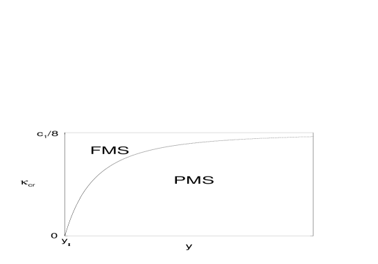
Figure 1: The generic phase diagram for the system (3) at strong Higgs-Majorana coupling; FMS and PMS are the strong coupling ferromagnetic (broken) and paramagnetic (symmetric) phases, respectively.

This confirms the indirect arguments of ref. [15].

Let us assume now that the system is within such a phase and consider what may happen to it there.

5 Within the PMS phase

Since the Higgs field fluctuates strongly in this phase, and $\langle\Phi\rangle=0$, standard methods of examination of such systems, working in the broken phases, is inapplicable here. We however still can get some idea of what may happen in this phase making use the method proposed in [20, 21].

Let us represent the Higgs field in (8) as

$$\Phi_{n}=\widetilde{\Phi}_{n}^{T}\widetilde{\Phi}_{n},$$ (47)

where the group valued field $\widetilde{\Phi}$, $\widetilde{\Phi}_{n}^{\dagger}\widetilde{\Phi}_{n}=1$, transforms under the gauge group as $\widetilde{\Phi}_{n}\rightarrow\widetilde{\Phi}_{n}g_{n}^{\dagger}$. Following the arguments of [20, 21], we assume that adequate nonzero parameter in the PMS phase is the link expectation value

$$z^{2}=\langle\widetilde{\Phi}^{\dagger}_{n}\widetilde{\Phi}_{n\pm\hat{\mu}}\rangle,\quad\langle\widetilde{\Phi}_{n}\rangle=\langle\widetilde{\Phi}^{\dagger}_{n}\rangle=0.$$ (48)

Further results will depend on the dynamical variables in terms of which the consideration is performed. Therefore we consider all the three possibilities.

1. Introduce the gauge group singlet fields

$$\widetilde{\chi}_{N_{s}}=z\widetilde{\Phi}\chi_{N_{s}},\quad\overline{\widetilde{\chi}}_{N_{s}}=z\overline{\chi}_{N_{s}}\widetilde{\Phi}^{\dagger}.$$ (49)

Then, with taking into account (48), the system (8) in the PMS phase at tree level can be described by the action

$$\widetilde{A}_{1}=\sum_{s,t\neq N_{s}}(\overline{\psi}_{s}\delta_{st}D\psi_{t}+\overline{\chi}_{s}\delta_{st}\overline{D}\chi_{t}+\overline{\psi}_{s}W^{-}_{st}\chi_{t}+\overline{\chi}_{s}W^{+}_{st}\psi_{t})$$ (50)

$$\qquad\qquad+\overline{\psi}_{N_{s}}D{\psi}_{N_{s}}+\overline{\psi}_{N_{s}}{\chi}_{N_{s}-1}+\overline{\chi}_{N_{s}-1}{\psi}_{N_{s}}$$ (51)

$$\qquad\qquad+\overline{\widetilde{\chi}}_{N_{s}}\overline{D}\widetilde{\chi}_{N_{s}}+\frac{y}{z^{2}}(\widetilde{\chi}_{N_{s}}^{T}\sigma_{2}\widetilde{\chi}_{N_{s}}+\overline{\widetilde{\chi}}_{N_{s}}\sigma_{2}\overline{\widetilde{\chi}}_{N_{s}}^{T}),$$ (52)

where we omit summation over four-dimensional indices. We see that in this case the massive neutral fermion $\widetilde{\chi}_{N_{s}}$ is decoupled, for the Wilson term at $s=N_{s}$ vanishes. This made $\widetilde{\chi}_{N_{s}}$ and $\psi_{N_{s}}$ naive, and although at the first glance this should not affect the chiral properties of the system, since both these fermions still have masses of the order of the cutoff, it turns out that it gives rise to species doubling of a massless mode. It is clearly seen from the structure of the fermion determinant, which in this case takes the form [cf. (39)]

$$Z_{1}=\mbox{Det}^{N_{s}+1}[D]\>\prod_{s=0}^{N_{s}-1}\mbox{Det}[B_{s}]\>\mbox{Det}^{1/2}[4\frac{y^{2}}{z^{4}}-D\overline{D}],$$ (53)

where the functions $B_{s}$ are determined in (42). Since $B_{s}\propto D^{-1}$, the determinant has zero at the corners of the Brillouine zone. So this scenario leads to the failure of the model.

2. Together with the neutral fields (49) one can also introduce the neutral fields

$$\widetilde{\psi}_{N_{s}}=z\widetilde{\Phi}\psi_{N_{s}},\quad\overline{\widetilde{\psi}}_{N_{s}}=z\overline{\psi}_{N_{s}}\widetilde{\Phi}^{\dagger}.$$ (54)

In terms of these variables the system in the PMS phase takes the form

$$\widetilde{A}_{2}=\sum_{s,t\neq N_{s}}(\overline{\psi}_{s}\delta_{st}D\psi_{t}+\overline{\chi}_{s}\delta_{st}\overline{D}\chi_{t}+\overline{\psi}_{s}W^{-}_{st}\chi_{t}+\overline{\chi}_{s}W^{+}_{st}\psi_{t})$$ (55)

$$\qquad\qquad+\overline{\widetilde{\psi}}_{N_{s}}D{\widetilde{\psi}}_{N_{s}}+\overline{\widetilde{\chi}}_{N_{s}}\overline{D}\widetilde{\chi}_{N_{s}}-\overline{\widetilde{\psi}}_{N_{s}}\widetilde{W}\widetilde{\chi}_{N_{s}}-\overline{\widetilde{\chi}}_{N_{s}}\widetilde{W}\widetilde{\psi}_{N_{s}}$$ (56)

$$\qquad\qquad+\frac{y}{z^{2}}(\widetilde{\chi}_{N_{s}}^{T}\sigma_{2}\widetilde{\chi}_{N_{s}}+\overline{\widetilde{\chi}}_{N_{s}}\sigma_{2}\overline{\widetilde{\chi}}_{N_{s}}^{T}),$$ (57)

where in the four-dimensional momentum space

$$\widetilde{W}=\frac{1}{z^{2}}(1-M)-\sum_{\mu}\left(\cos p_{\mu}-\frac{1}{z^{2}}\right).$$ (58)

In this case the slice $s=N_{s}$ decouples from the rest of the lattice, so that one has massive neutral fermions at $s=N_{s}$ and the original massless model on the rest of the lattice. The neutral fermions $\widetilde{\psi}_{N_{s}}$, $\widetilde{\chi}_{N_{s}}$ can still be made massless, by setting the domain wall mass to $M=5-4z^{2}$, but this does not rescue the situation with the rest of the lattice. So in this case the model fails, too.

3. Finally, in terms of the singlet fields like (49) and (54) introduced at all $s$, the action reads as

$$\widetilde{A}_{3}=\sum_{st}(\overline{\widetilde{\psi}}_{s}\delta_{st}D\widetilde{\psi}_{t}+\overline{\widetilde{\chi}}_{s}\delta_{st}\overline{D}\widetilde{\chi}_{t}+\overline{\widetilde{\psi}}_{s}\widetilde{W}^{-}_{st}\widetilde{\chi}_{t}+\overline{\widetilde{\chi}}_{s}\widetilde{W}^{+}_{st}\widetilde{\psi}_{t})$$ (59)

$$\qquad+\frac{y}{z^{2}}(\widetilde{\chi}_{N_{s}}^{T}\sigma_{2}\widetilde{\chi}_{N_{s}}+\overline{\widetilde{\chi}}_{N_{s}}\sigma_{2}\overline{\widetilde{\chi}}_{N_{s}}^{T}),$$ (60)

where

$$\widetilde{W}^{\pm}_{st}=\frac{1}{z^{2}}\delta_{s\pm 1\,t}-\delta_{st}\widetilde{W}.$$ (61)

We see that these system is equivalent to that considered in the previous section, only if $z=1$. However one can hardly expect that it is so on the ground of the estimations of $z^{2}$ in pure scalar models [12, 14]. For instance, in $O(2)$ and $O(4)$ models it has been found $z^{2}\simeq 0.19$. Therefore our previous analysis is not directly applicable to this system. However we can made some qualitative conclusions about the effects of such renormalization.

An analysis similar to that of the beginning of the previous section, shows that in the continuum case, when the Wilson term is equal to zero, $z$ simply renormalizes the masses of the massive excitations: now they become $1/z^{2}$, rather than 1. The situation on the lattice is more complicated. Indeed, making the small $p$ expansion in (61) one can see that the role of the factor $1-M$, which provides the localization of the massless states at the boundaries, now is played by $z$ dependent combination $5-4z^{2}-M$, that may considerably shift the range of admissible values of $M$. This requires a priori knowledge of the $z$, that complicates considerably the numerical study of such models. But the main problem in this variant is that all the fermions in the system now are neutral.

The question of which of these scenarios is realized actually in the system requires special investigation, and the answer may depend on the strength of the Wilson parameter $r$, set to 1 in this paper, as well as on the couplings $y$ and $\kappa$. However none of them leads to the chiral spectrum of charged, i.e. gauge non-singlet, fermions which one tends to describe. So we can conclude that in this respect the domain wall fermions have no appreciable advantages compared with the four dimensional Wilson fermions.

6 Summary and prospects

The lattice boundary formulation of chiral fermions with Majorana mass introduced for the field $\chi$ on the boundary $s=N_{s}$ indeed yields the low-lying chiral spectrum at the tree level: there exists only one massless left-handed fermion $\psi$ localized at the boundary $s=0$. Our results also show that effects caused by the introduction of such Majorana mass is strongly suppressed in physical sector. For instance, the fermion number violation for the $\psi$ is suppressed exponentially as the size of the fifth dimension $N_{s}$ increases.

Since the Majorana mass does not break the gauge invariance for real representations of the gauge group, the most immediate implementation of such systems is the lattice formulation of the $N=1$ supersymetric models [17]. Our results speaks in favour of this idea, since the exponential suppression of the undesirable effects in the physical sector is an indication that the problem of fine tuning can be avoided in such a formulation, at least in the perturbation theory. This however should be demonstrated explicitly, and this work now is in progress.

The prospect for chiral gauge theories is less certain, for they have to employ the generalized Higgs mechanism in the PMS phase. Although we have demonstrated that the PMS phase can exist in these models, their possible dynamics within such a phase does not give a ground for optimism. Indeed, we argued that the spectrum of charge fermions within the PMS phase is vectorlike, and that only spectrum of the neutral states, by a certain tuning of the domain wall mass, can be made chiral. Thus the crucial question is what is the gauge interactions of such neutral chiral states. Previous studies of similar states appearing in the models with the Wilson-Yukawa couplings give a strong evidence that such states in the continuum limit become non-interacting [11, 12, 13, 14]. It is this point that leads to very plausible failure of those models, as well as the models with multifermion couplings [22]. Such screening of the chiral charges appears to be an universal phenomenon pursuing any models within the PMS phase. Therefore we consider this point as the main problem on the way of implementation of the domain wall fermions to exactly gauge invariant nonperturbative formulation of chiral gauge theories.

Acknowledgements

S.V.Z. is grateful to the staff of the Center for Computational Physics, where this work has been done, and particularly to Y. Iwasaki and A. Ukawa, for their kind hospitality. S.A. was supported in part by the Grants-in-Aid of the Ministry of Education (No.08640350); S.V.Z. was supported by “COE Foreign Researcher Program” of the Ministry of Education of Japan and by the Russian Basic Research Fund under the grant 95-02-03868a.

References

• [1] H. B. Nielsen and M. Ninomiya, Nucl. Phys. B 185 (1981) 20; B 195 (1981) 541 (E); B 193 (1981) 173; Phys. Lett. 105B (1981) 219.
• [2] K. G. Wilson, in New phenomena in subnuclear physics, edited by A. Zichichi (Plenum Press, New York, 1996), p. 69.
• [3] D. B. Kaplan, Phys. Lett. B 288 (1992) 342; Nucl. Phys. B (Proc. Suppl.) 30 (1993) 597.
• [4] Y. Shamir, Nucl. Phys. B 406 (1993) 90.
• [5] K. Jansen, Phys. Rept. 273 (1996) 1.
• [6] R. Narayanan and H. Neuberger, Phys. Lett. B 302 (1993) 62;
S. A. Frolov and A. A. Slavnov, Nucl. Phys. B 411 (1994) 647.
• [7] R. Narayanan and H. Neuberger, Nucl. Phys. B 412 (1994) 574; B 443 (1995) 305.
• [8] D. N. Petcher, Nucl. Phys. B (Proc. Suppl.) 30 (1993) 50.
• [9] Y. Shamir, Nucl. Phys. B (Proc. Suppl.) 47 (1996) 212.
• [10] J. Shigemitsu, Nucl. Phys. B (Proc. Suppl.) 20 (1991) 515.
• [11] M. F. L. Golterman, D. N. Petcher, and J. Smit, Nucl. Phys B 370 (1992) 51.
• [12] W. Bock, A. K. De, and J. Smit, Nucl. Phys. B388 (1992) 243.
• [13] M. F. L. Golterman, D. N. Petcher, and E. Rivas, Nucl. Phys. B 377 (1992) 405.
• [14] S. Aoki, H. Hirose, and Y. Kikukawa, Int. J. Modern Phys. A9 (1994) 4129.
• [15] M. Creutz, M. Tytgat, C. Rebbi, and S-S. Xue, hep-lat/9612017.
• [16] E. Eichten and Preskill, Nucl. Phys. B 268 (1986) 179.
• [17] J. Nishimura, hep-lat/9701013.
• [18] S. Aoki and H. Hirose, Phys. Rev. D 49 (1994) 2604.
• [19] S. Tominaga and S. V. Zenkin, Phys. Rev. D 50 (1994) 3387;
S. V. Zenkin, Phys. Rev. D 53 (1996) 6674.
• [20] J. Smit, Nucl. Phys. B (Proc. Suppl.) 9 (1989) 579; 17 (1990) 3.
• [21] I-H. Lee, Nucl. Phys. B (Proc. Suppl.) 17 (1990) 457;
S. Aoki, I-H. Lee, and R.E. Shrock, Nucl. Phys. B355 (1991) 383.
• [22] M. F. L. Golterman, D. N. Petcher, and E. Rivas, Nucl. Phys. B 395 (1993) 596.