WUB 97-14
HLRZ 1997_16
Light Quark Masses with Dynamical Wilson Fermions

Abstract

We determine the masses of the light and the strange quarks in the $\overline{MS}$-scheme using our high-statistics lattice simulation of QCD with dynamical Wilson fermions. For the light quark mass we find $m^{\rm light}_{\overline{MS}}(2\,{\sf GeV})=2.7(2)\,{\sf MeV}$, which is lower than in quenched simulations. For the strange quark, in a sea of two dynamical light quarks, we obtain $m^{\rm strange}_{\overline{MS}}(2\,{\sf GeV})=140(20)\,{\sf MeV}$.

1 Introduction

The masses of $u$, $d$, and $s$ quarks constitute fundamental parameters of the Standard Model. Phenomenologically, however, they remain among the most poorly known quantities within its scenario.

While lowest order chiral perturbation theory offers a fairly easy access to the determination of ratios of quark masses from the empirical mesonic spectrum[1], one has to apply much more meticulous techniques, such as QCD sum rules[2] or lattice QCD[3, 4], in order to arrive at absolute values. At this stage, however, these two methods appear to lead to contradictory results.

In practice, both of these approaches carry their specific merits and shortcomings. While the sum rule results are sensitive to the choice of parametrizations, as elaborated in ref.[5], the lattice results have been established so far for pure gluon dynamics only[3, 4].

It is therefore of considerable interest to study the dynamical effects of vacuum fluctuations, originating from light quarks, onto light quark properties such as their masses. This holds in particular for Wilson-like discretizations of fermions which, unlike staggered fermions, are free of flavour symmetry violations on the lattice. Until recently, however, computing resources and techniques were too limited to allow for the generation of reliable samples of vacuum configurations with appropriate statistics. Nevertheless, a recent rough analysis of world data seems to suggest[4] that unquenching from $N_{f}=0$ to $N_{f}=2$ might have a sizeable impact on the value of the light and strange quark masses, lowering them by as much as 50 %.

In this letter, we present a lattice analysis for the light and strange quark masses based on our measurements of the pseudoscalar and vector mesons determined in a sea of two degenerate dynamical quarks. We have generated three sets of gauge configurations at three sea-quark masses but at the same coupling; each set comprises 200 independent gauge configurations. Good signals in the autocorrelation functions and the use of a blocking method give us confidence as to the reliability of the quoted errors.

The masses of the light and the strange quark are extracted from the meson data by fixing two mass ratios, ${M_{\pi}\over M\rho}$ for the light and one of ${M_{\phi}\over M\rho}$, ${M_{K}\over M\rho}$ or ${M_{K^{*}}\over M\rho}$ for the strange; the lattice spacing is obtained from $M_{\rho}$.

We identify the dynamical quarks with the degenerate doublet of isopsin symmetric quarks, $u$ and $d$, called light quark in the following. Thus, using our data for the pseudoscalar and the vector at the three sea-quarks, we can extract the mass of the light quark in a sea of light quarks.

To simulate the strange quark we need to introduce valence quarks that are unequal to the dynamical quarks: at each sea-quark we evaluate meson masses with strange valence quarks and perform an extrapolation of these masses to the physical sea of light quarks. This procedure allows us to calculate the masses of the $K$, $K^{*}$ and the $\phi$ with a dynamical light quark(for $K$ and $K^{*}$) and strange quarks in a sea of light quarks.

The definition of a strange quark mass in a sea of light quarks requires an analysis of lattice data in terms of sea and valence quark masses, for which we describe a suitable parametrization in section 3. As an aside, we also comment on a possible flaw in the extraction of quark masses from quenched data with Wilson-like fermions.

2 Simulation details

$\beta_{\rm dyn}=5.6$, $N_{f}=2$, $16^{3}\times 32$
$\kappa_{\rm sea}$	0.156	0.1570	0.1575
number of configurations	200	200	200
$\kappa_{\rm V}-\kappa_{\rm V}$ combinations	15	15	15
$\beta_{\rm quenched}=6.0$, $16^{3}\times 32$
number of configurations: 200
$\kappa_{\rm V}-\kappa_{\rm V}$ combinations: 15

Table 1: Simulation details.

In table 1 we show the parameters of our simulation. In addition to the dynamical simulation we performed a quenched study at the matching quenched coupling to enable a direct comparison of full and quenched QCD.

At each of our three sea-quark values, characterized by the hopping parameters $\kappa_{\rm sea}$, we have investigated zero-momentum two-point functions,

$$C_{AB}(t)=\sum_{\vec{x}}\langle 0|\chi_{A}^{\dagger}(0)\chi_{B}(x)|0\rangle\;,$$ (1)

for the pseudoscalar and vector particles, $\chi_{PS}(x)=\bar{q}^{\prime}(x)\gamma^{5}q(x)$ and $\chi^{\mu}_{V}(x)=\bar{q}^{\prime}(x)\gamma^{\mu}q(x)$. We combined light-quark propagators with hopping parameters equal and different to that of the corresponding sea-quark, allowing for fifteen mass estimates per sea-quark. We use the gauge-invariant Wuppertal-smearing procedure[6] to calculate smeared-local and smeared-smeared correlators (with smearing parameter $\alpha=4$ and with 50 iterations). Both types of smearing are used to obtain mass-estimates by performing a simultaneous single-exponential fit to the data on time-slices 10-15. Details will be given in [7].

In ref.[8] we will present a detailed auto-correlation analysis. We found integrated auto-correlation times, $\tau_{\rm int}$, for the masses to lie around 25 HMC time-units with a slight increase towards lighter sea-quarks. We have therefore chosen to calculate propagators on configurations separated by 25 HMC trajectories. To determine by how many units of $\tau_{\rm int}$ the measurements need to be separated to achieve complete decorrelation we performed a blocking analysis and plotted the error as a function of the blocking size. At block size 6 (for $\kappa_{\rm sea}=0.156$ and $0.157$) and 7 (at $\kappa_{\rm sea}=0.1575$) we find the jackknife errors of the error to run into plateaus. Consequently, these are the errors we will quote in the following. A similar analysis for our quenched data shows no increase in error with the blocksize (quenched configurations are generated with an overrelaxed Cabbibo-Marinari heatbath update and are separated by 250 sweeps).

Errors (on the blocked data) are obtained using the bootstrap procedure. They correspond to 68 % confidence limits of the distribution obtained from 250 bootstrap samples.

3 Results - light and strange quarks

The light quark mass is extracted by matching the ratio:

$${m_{\rm PS}\over m_{\rm V}}={M_{\pi}\over M_{\rho}}=0.1785\,,$$ (2)

using data with (degenerate) valence quarks equal to the sea-quarks. Generically, we call this data $m_{\sf ss}$. Owing to the fact that we have but three different sea-quarks,

$$m^{\rm sea}={1\over 2}\left({1\over\kappa_{\rm sea}}-{1\over\kappa_{\rm sea}^{c}}\right)\;,$$ (3)

we use linear extrapolations in the lattice quark mass:

$$m_{\rm PS,{\sf ss}}^{2} = c\left({1\over\kappa_{\rm sea}}-{1\over\kappa_{\rm sea}^{c}}\right)\;,$$ (4)

$$m_{\rm V,{\sf ss}} = m^{\rm crit}+bm_{\rm PS,{\sf ss}}^{2}\;.$$

Figure 1: $m_{\rm PS,{\sf ss}}^{2}$ (left) as a function of ${1\over\kappa_{\rm sea}}$ and $m_{\rm V,{\sf ss}}$ as a function of $m^{\rm sea}$ (in lattice units).

These fits, which we call “symmetric”, are shown in figure 1. We find the pseudoscalar mass to be extremely well matched by the linear ansatz ($\chi^{2}/{\sf d.o.f}=0.002$), whereas the vector masses may exhibit some downward curvature ($\chi^{2}/{\sf d.o.f}=1.1$). We find:

$$\kappa_{\rm sea}^{c}=0.15846(5)\;\;\;\;\kappa_{\rm sea}^{\rm light}=0.15841(5)\;,$$ (5)

$$m^{\rm light}={1\over 2}\left({1\over\kappa_{\rm sea}^{\rm light}}-{1\over\kappa_{\rm sea}^{c}}\right)=0.00088(6)\;.$$ (6)

The corresponding lattice spacings from the rho are:

$$a^{-1}_{\rho} = 2.35(6)\;{\sf GeV}\;\;\;\;{\rm at}\;\;\kappa_{\rm sea}^{c},$$ (7)

$$a^{-1}_{\rho} = 2.33(6)\;{\sf GeV}\;\;\;\;{\rm at}\;\;\kappa_{\rm sea}^{\rm light}.$$ (8)

We use the latter value to convert to physical units in the $\overline{MS}$-scheme according to:

$$m_{\overline{MS}}(\mu)=Z_{M}(\mu a)m^{\rm sea}a^{-1}_{\rho}\;,$$ (9)

with $Z_{M}(\mu a)$ calculated in boosted 1-loop perturbation theory [12, 13] and run the values to 2 ${\sf GeV}$. Throughout, we allow for a 3 % uncertainty in $Z_{M}$. As a result we find:

$$m^{\rm light}_{\overline{MS}}(2\,{\sf GeV}) = 2.7(2)\,{\sf MeV}\;.$$ (10)

As we have outlined in the introduction, the treatment of the strange quark within the context of an $N_{f}=2$ simulation requires the computation of mesons with valence quarks unequal to the dynamical light sea-quarks. In addition to $m_{\sf ss}$ we introduce the following generic notation:

• $m_{\sf sv}$ - one valence quark is identical to the sea-quark.

• $m_{\sf vv}$ - neither valence quark is identical to the sea-quark.

Furthermore, we define an effective $\kappa$ through ${1\over\kappa^{\rm eff}_{\rm v}}={1\over 2}\left({1\over\kappa^{1}_{\rm v}}+{1\over\kappa^{2}_{\rm v}}\right)$, where $\kappa^{1}_{\rm v}$ and $\kappa^{2}_{\rm v}$ refer to valence quarks in a meson.

In principle, we can fit $m_{\rm PS,{\sf vv}}^{2}$ and $m_{\rm PS,{\sf sv}}^{2}$ to independent linear functions in ${1\over\kappa_{\rm sea}}$ and ${1\over\kappa_{\rm V}}$,

$$m_{\rm PS,{\sf vv}}^{2} = c_{1}+c_{2}{1\over\kappa_{\rm V}}+c_{3}{1\over\kappa_{\rm sea}}+\cdots\;,$$ (11)

$$m_{\rm PS,{\sf sv}}^{2} = c_{1}^{\prime}+c_{2}^{\prime}{1\over\kappa_{\rm V}}+c_{3}^{\prime}{1\over\kappa_{\rm sea}}+\cdots\;.$$ (12)

However, from the requirement that all parametrizations must converge smoothly into each other on the symmetric line, $\kappa_{\rm sea}=\kappa_{\rm V}$, the number of independent parameters can be substantially reduced. For $m_{\rm PS,{\sf vv}}^{2}$, for example, one finds $c_{2}+c_{3}=c$ and $c_{1}=-{c\over\kappa_{\rm sea}^{c}}$. In particular, at the critical point $m_{\rm PS,{\sf ss}}^{2}=m_{\rm PS,{\sf sv}}^{2}=m_{\rm PS,{\sf vv}}^{2}=0$, valence and sea quark masses must be identical: $\kappa_{\rm V}^{c}(\kappa_{\rm sea}^{c})=\kappa_{\rm sea}^{c}$. This simplifies the mass equations to:

$$m_{\rm PS,{\sf vv}}^{2} = -c{1\over\kappa_{\rm sea}^{c}}+c_{3}{1\over\kappa_{\rm sea}}+{1\over\kappa_{\rm V}}\left(c-c_{3}\right)\;,$$ (13)

$$m_{\rm PS,{\sf sv}}^{2} = -c{1\over\kappa_{\rm sea}^{c}}+c_{3}^{\prime}{1\over\kappa_{\rm sea}}+{1\over\kappa_{\rm V}}\left(c-c_{3}^{\prime}\right)\;.$$ (14)

Defining a bare valence quark mass with respect to $\kappa_{\rm sea}^{c}$ as:

$$m^{\rm V}={1\over 2}\left({1\over\kappa_{\rm v}^{\rm eff}}-{1\over\kappa_{\rm sea}^{c}}\right)\;\;,$$ (15)

we can summarize the combined parametrization as follows[10]:

$$\left(\begin{array}[]{c}m_{\rm PS,{\sf ss}}^{2}\\ m_{\rm PS,{\sf sv}}^{2}\\ m_{\rm PS,{\sf vv}}^{2}\end{array}\right) = \left(\begin{array}[]{cc}2c&0\\ c+c_{13}&c-c_{13}\\ c_{34}&2c-c_{34}\end{array}\right)\left(\begin{array}[]{c}m^{\rm sea}\\ m^{\rm V}\end{array}\right)\;\;,$$ (24)

where the variables $c_{34}=2c_{3}$ and $c_{13}=2c_{3}^{\prime}-c$ have been introduced. Similarily, the vector-data can be parametrized as:

$$\left(\begin{array}[]{c}m_{\rm V,{\sf ss}}\\ m_{\rm V,{\sf sv}}\\ m_{\rm V,{\sf vv}}\end{array}\right) = m^{\rm crit}\,+\,b\left(\begin{array}[]{c}m_{\rm PS,{\sf ss}}^{2}\\ m_{\rm PS,{\sf sv}}^{2}\\ m_{\rm PS,{\sf vv}}^{2}\end{array}\right)\;\;.$$ (31)

Once the fit parameters $c$, $c_{13}$, $c_{34}$ and $\kappa_{\rm sea}^{c}$ for the pseudoscalar and additionally $m^{\rm crit}$ and $b$ for the vector particle have been determined, we can calculate all quark masses; no additonal fitting is needed.

Figure 2: Simultaneous fit of all pseudoscalar data to eq. 24. The vector data are fit to a semi-constrained form (see text). Symbols: $*=m_{\sf ss}\;-\!\!-$; $\Diamond=m_{\sf sv}\;-\cdot\;-$; $\Box=m_{\sf vv}\;-\,-$. All plots in lattice units.

Figure 2 (left plot) shows such a combined linear extrapolation of all the pseudoscalar data with the ansatz of eq. 24. The data are nicely fitted by this parametrization ($\chi^{2}/{\sf d.o.f}=4.4/23$). A constrained fit to the vector-data with eq. 31 turns out to be more difficult; we find a $\chi^{2}/{\sf d.o.f}=50/25$, fit-parameters are given in table 2. A much better $\chi^{2}/{\sf d.o.f}$ for the vector particle can be achieved by a semi-constrained fit in which only $\kappa_{\rm sea}^{c}$, as given in eq. 5, is held fixed, but the parameters $c$, $c_{13}$ and $c_{34}$ are allowed to vary. This is shown in figure 2 on the r.h.s.. The data for $m_{\sf sv}$ and $m_{\sf vv}$ are best fit for those data points of $m_{\sf ss}$ which match eq. 4 well.

Before we proceed to extract the strange quark mass, let us check for the consistency of the method by using the combined equation to determine the light quark mass and by comparing with our previous result, eq. 6.

$\kappa_{\rm sea}^{c}$	$\kappa_{\rm sea}^{\rm light}$	$c$	$c_{13}$	$c_{34}$	$b$	$m^{\rm crit}$	$\chi^{2}/{\sf d.o.f}$
symmetric fit to $m_{\rm PS,{\sf ss}}^{2}$ and $m_{\rm V,{\sf ss}}$
$0.15846\raisebox{0.80002pt}{\scriptsize{$\begin{array}[]{@{}l@{}}\makebox[15.0pt][c]{$+$}\makebox[3.85002pt][r]{5}\\[-0.35002pt] \makebox[15.0pt][c]{$-$}\makebox[3.85002pt][r]{5}\end{array}$}}$	$0.15841\raisebox{0.80002pt}{\scriptsize{$\begin{array}[]{@{}l@{}}\makebox[15.0pt][c]{$+$}\makebox[3.85002pt][r]{5}\\[-0.35002pt] \makebox[15.0pt][c]{$-$}\makebox[3.85002pt][r]{5}\end{array}$}}$	$1.99\raisebox{0.80002pt}{\scriptsize{$\begin{array}[]{@{}l@{}}\makebox[15.0pt][c]{$+$}\makebox[3.85002pt][r]{6}\\[-0.35002pt] \makebox[15.0pt][c]{$-$}\makebox[3.85002pt][r]{6}\end{array}$}}$	-	-	$1.02\raisebox{0.80002pt}{\scriptsize{$\begin{array}[]{@{}l@{}}\makebox[15.0pt][c]{$+$}\makebox[3.85002pt][r]{4}\\[-0.35002pt] \makebox[15.0pt][c]{$-$}\makebox[3.85002pt][r]{6}\end{array}$}}$	$0.328\raisebox{0.80002pt}{\scriptsize{$\begin{array}[]{@{}l@{}}\makebox[15.0pt][c]{$+$}\makebox[3.85002pt][r]{10}\\[-0.35002pt] \makebox[15.0pt][c]{$-$}\makebox[3.85002pt][r]{8}\end{array}$}}$	$0.0024$, $1.1$
constrained fit to eq. 24 and eq. 31
$0.15845\raisebox{0.80002pt}{\scriptsize{$\begin{array}[]{@{}l@{}}\makebox[15.0pt][c]{$+$}\makebox[3.85002pt][r]{5}\\[-0.35002pt] \makebox[15.0pt][c]{$-$}\makebox[3.85002pt][r]{5}\end{array}$}}$	$0.15841\raisebox{0.80002pt}{\scriptsize{$\begin{array}[]{@{}l@{}}\makebox[15.0pt][c]{$+$}\makebox[3.85002pt][r]{5}\\[-0.35002pt] \makebox[15.0pt][c]{$-$}\makebox[3.85002pt][r]{4}\end{array}$}}$	$1.98\raisebox{0.80002pt}{\scriptsize{$\begin{array}[]{@{}l@{}}\makebox[15.0pt][c]{$+$}\makebox[3.85002pt][r]{6}\\[-0.35002pt] \makebox[15.0pt][c]{$-$}\makebox[3.85002pt][r]{6}\end{array}$}}$	$0.88\raisebox{0.80002pt}{\scriptsize{$\begin{array}[]{@{}l@{}}\makebox[15.0pt][c]{$+$}\makebox[3.85002pt][r]{6}\\[-0.35002pt] \makebox[15.0pt][c]{$-$}\makebox[3.85002pt][r]{6}\end{array}$}}$	$1.7\raisebox{0.80002pt}{\scriptsize{$\begin{array}[]{@{}l@{}}\makebox[15.0pt][c]{$+$}\makebox[3.85002pt][r]{1}\\[-0.35002pt] \makebox[15.0pt][c]{$-$}\makebox[3.85002pt][r]{1}\end{array}$}}$	$1.02\raisebox{0.80002pt}{\scriptsize{$\begin{array}[]{@{}l@{}}\makebox[15.0pt][c]{$+$}\makebox[3.85002pt][r]{3}\\[-0.35002pt] \makebox[15.0pt][c]{$-$}\makebox[3.85002pt][r]{5}\end{array}$}}$	$0.329\raisebox{0.80002pt}{\scriptsize{$\begin{array}[]{@{}l@{}}\makebox[15.0pt][c]{$+$}\makebox[3.85002pt][r]{8}\\[-0.35002pt] \makebox[15.0pt][c]{$-$}\makebox[3.85002pt][r]{6}\end{array}$}}$	$4.4/23$, $50/25$
semi-constrained fit to eq. 31
$\kappa_{\rm sea}^{c}$	$\kappa_{\rm sea}^{\rm light}$	$c^{\sf rho}$	$c_{13}^{\sf rho}$	$c_{34}^{\sf rho}$	$b$	$m^{\rm crit}$	$\chi^{2}/{\sf d.o.f}$
$0.15845\raisebox{0.80002pt}{\scriptsize{$\begin{array}[]{@{}l@{}}\makebox[15.0pt][c]{$+$}\makebox[3.85002pt][r]{5}\\[-0.35002pt] \makebox[15.0pt][c]{$-$}\makebox[3.85002pt][r]{5}\end{array}$}}$	$0.15841\raisebox{0.80002pt}{\scriptsize{$\begin{array}[]{@{}l@{}}\makebox[15.0pt][c]{$+$}\makebox[3.85002pt][r]{5}\\[-0.35002pt] \makebox[15.0pt][c]{$-$}\makebox[3.85002pt][r]{5}\end{array}$}}$	$2.08\raisebox{0.80002pt}{\scriptsize{$\begin{array}[]{@{}l@{}}\makebox[15.0pt][c]{$+$}\makebox[3.85002pt][r]{10}\\[-0.35002pt] \makebox[15.0pt][c]{$-$}\makebox[3.85002pt][r]{12}\end{array}$}}$	$1.06\raisebox{0.80002pt}{\scriptsize{$\begin{array}[]{@{}l@{}}\makebox[15.0pt][c]{$+$}\makebox[3.85002pt][r]{9}\\[-0.35002pt] \makebox[15.0pt][c]{$-$}\makebox[3.85002pt][r]{12}\end{array}$}}$	$2.1\raisebox{0.80002pt}{\scriptsize{$\begin{array}[]{@{}l@{}}\makebox[15.0pt][c]{$+$}\makebox[3.85002pt][r]{2}\\[-0.35002pt] \makebox[15.0pt][c]{$-$}\makebox[3.85002pt][r]{2}\end{array}$}}$	-	$0.326\raisebox{0.80002pt}{\scriptsize{$\begin{array}[]{@{}l@{}}\makebox[15.0pt][c]{$+$}\makebox[3.85002pt][r]{9}\\[-0.35002pt] \makebox[15.0pt][c]{$-$}\makebox[3.85002pt][r]{7}\end{array}$}}$	$4.4/23$, $6.3/23$

Table 2: Fit results from constrained (equations 24 and 31) as well as from symmetric fits to the pseudoscalar and vector and the values of $\kappa_{\rm sea}^{c}$ and $\kappa_{\rm sea}^{\rm light}$.

Table 2 shows that all three fits lead to stable values of $m^{\rm crit}$ as well as $\kappa_{\rm sea}^{c}$ and $\kappa_{\rm sea}^{\rm light}$. This gives us confidence in our method of choice: we employ a semi-constrained fit to extract the strange quark mass.

The data $m_{\sf sv}$ and $m_{\sf vv}$ are used as follows:

• Determine $\kappa^{\rm strange}$ from $m_{\sf sv}$ by matching

  $${m_{\rm V,{\sf sv}}(\kappa_{\rm sea}^{\rm light},\kappa^{\rm strange})\over m_{\rm V,{\sf ss}}(\kappa_{\rm sea}^{\rm light})}={M_{K^{*}}\over M_{\rho}}=1.16\;,$$ (32)

  where $\kappa_{\rm sea}^{\rm light}$ is given by eq. 5. Alternatively, the $K$ can be used.

• Determine $\kappa^{\rm strange}$ from $m_{\sf sv}$ by matching

  $${m_{V_{1},{\rm vv}}(\kappa_{\rm sea}^{\rm light},\kappa^{\rm strange})\over m_{V_{2},{\rm ss}}(\kappa_{\rm sea}^{\rm light})}={M_{\phi}\over M_{\rho}}=1.326\;.$$ (33)

Table 3 shows the results for all three particles employed. Good agreement is found between the $\phi$ and the $K^{*}$, whereas the $K$ favours a slightly larger $\kappa^{\rm strange}$. This is illustrated in figure 3, where ${1\over\kappa^{\rm strange}}$ is plotted as a funtion of ${1\over\kappa_{\rm sea}}$.

To check for a systematic error we have also tried constrained fits to the vector particle. Encouragingly, we find only negligible change (see table 3).

Our final value is:

$$\kappa^{\rm strange}=0.15615(20)^{\sf stat}(20)^{\sf syst}\;,$$ (34)

where the systematic error covers the spread for all three particles. The conversion yields:

$$m^{\rm strange}_{\overline{MS}}(2\,{\sf GeV})=140(20)\,{\sf MeV}\;.$$ (35)

Figure 3: Chiral behaviour of ${1\over\kappa^{\rm strange}}$, as determined from $K^{*}$($\Box$), $\phi$($\bigcirc$) and the $K$($\Diamond$). The strange quark mass is calculated with the light quark mass fixed to its physical value. At the very left we plot the value for a strange quark in a strange sea. Lines are calculated from eq. 24 and eq. 31.

Before we turn to a discussion of our results, we comment on a method which has been proposed for the extraction of $\kappa^{\rm strange}$ with 2 dynamical quarks (see [4], for example). It circumvents the introduction of valence quarks unequal to the dynamical quarks and determines $\kappa^{\rm strange}$ by matching the ratio ${M_{\phi}\over M_{\rho}}$ using the symmetric fit only. Adopting this procedure, one finds $\kappa^{\rm strange}=0.15709\raisebox{0.80002pt}{\scriptsize{$\begin{array}[]{@{}l@{}}\makebox[15.0pt][c]{$+$}\makebox[3.85002pt][r]{8}\\[-0.35002pt] \makebox[15.0pt][c]{$-$}\makebox[3.85002pt][r]{12}\end{array}$}}$ and $m^{\rm strange}_{\overline{MS}}(2\,{\sf GeV})=80(8)\,{\sf MeV}$; this point is shown on the very left in figure 3. However, this method implies that the $\phi$ mass is measured with strange valence quarks in a sea of strange quarks. One would prefer the mass to be determined in a sea of light quarks, at which, naively, one expects the effects of dynamical sea-quarks to be more pronounced. It is interesting to see that the effect of light sea-quarks is fairly significant: the $\phi$, when measured in a sea of strange quarks, yields the largest of all estimates for $\kappa^{\rm strange}$.

particle	$\kappa^{\rm strange}$ constrained	$\kappa^{\rm strange}$ semi-constrained
$K$	$0.1564\raisebox{0.80002pt}{\scriptsize{$\begin{array}[]{@{}l@{}}\makebox[15.0pt][c]{$+$}\makebox[3.85002pt][r]{2}\\[-0.35002pt] \makebox[15.0pt][c]{$-$}\makebox[3.85002pt][r]{1}\end{array}$}}$	$0.1565\raisebox{0.80002pt}{\scriptsize{$\begin{array}[]{@{}l@{}}\makebox[15.0pt][c]{$+$}\makebox[3.85002pt][r]{2}\\[-0.35002pt] \makebox[15.0pt][c]{$-$}\makebox[3.85002pt][r]{2}\end{array}$}}$
$K^{*}$	$0.1561\raisebox{0.80002pt}{\scriptsize{$\begin{array}[]{@{}l@{}}\makebox[15.0pt][c]{$+$}\makebox[3.85002pt][r]{1}\\[-0.35002pt] \makebox[15.0pt][c]{$-$}\makebox[3.85002pt][r]{2}\end{array}$}}$	$0.1559\raisebox{0.80002pt}{\scriptsize{$\begin{array}[]{@{}l@{}}\makebox[15.0pt][c]{$+$}\makebox[3.85002pt][r]{1}\\[-0.35002pt] \makebox[15.0pt][c]{$-$}\makebox[3.85002pt][r]{2}\end{array}$}}$
$\phi$	$0.1561\raisebox{0.80002pt}{\scriptsize{$\begin{array}[]{@{}l@{}}\makebox[15.0pt][c]{$+$}\makebox[3.85002pt][r]{1}\\[-0.35002pt] \makebox[15.0pt][c]{$-$}\makebox[3.85002pt][r]{2}\end{array}$}}$	$0.1559\raisebox{0.80002pt}{\scriptsize{$\begin{array}[]{@{}l@{}}\makebox[15.0pt][c]{$+$}\makebox[3.85002pt][r]{1}\\[-0.35002pt] \makebox[15.0pt][c]{$-$}\makebox[3.85002pt][r]{1}\end{array}$}}$

Table 3: Collection of results for $\kappa^{\rm strange}$.

4 Discussion

Our results

$$\left.\begin{array}[]{c}m^{\rm light}_{\overline{MS}}(2\,{\sf GeV})=2.7(2)\,{\sf MeV}\\ m^{\rm strange}_{\overline{MS}}(2\,{\sf GeV})=140(20)\,{\sf MeV}\end{array}\right\} \;\;\;\;\mbox{{\rm 2 dynamical light quarks}}\;,$$ (38)

are to be compared to the analogous quenched values at corresponding $\beta_{\rm quenched}=6.0$:

$$\left.\begin{array}[]{c}m^{\rm light}_{\overline{MS}}(2\,{\sf GeV})=5.5(5)\,{\sf MeV}\\ m^{\rm strange}_{\overline{MS}}(2\,{\sf GeV})=166(15)\,{\sf MeV}\end{array}\right\} \;\;\;\;\mbox{{\rm quenched}}\;.$$ (41)

Errors due to the finite lattice spacing and the finite volume are not included in (38) and (41).

Compared to the quenched result, which is in good agreement with previous lattice calculations[4], we observe a much smaller dynamical light quark mass, whereas the strange masses are compatible within errors. Our dynamical result for the quark mass ratio, $m^{\rm strange}/m^{\rm light}\approx 52$, differs significantly from chiral perturbation theory estimates[1] or sum rule results[2]. This may be due to the fact that the effects of strange sea quarks can only be partially accounted for in an $N_{f}=2$ simulation.

We note that an extrapolation of quenched quark masses to $a=0$ yields much smaller values than eq. 41, $m^{\rm light}=3.4(5)$ and $m^{\rm strange}=100(23)$[4]. Nevertheless, the ratio $m^{\rm strange}/m^{\rm light}$ from quenched simulations is fairly independent of the lattice spacing $a$. This may be different in full QCD, as cutoff effects could show up differently in sea and valence quarks. Dynamical results at other couplings are needed before one can compare results in the $a=0$ limit.

To understand the drop in the mass of the light quark from $N_{f}=0$ to $N_{f}=2$ at fixed coupling we have analysed our dynamical data in a manner suggested by quenched lattice simulations. To this end, we have defined a quark mass at fixed sea-quark through:

$$m^{\rm V}={1\over 2}({1\over\kappa_{\rm v}^{\rm eff}}-{1\over\kappa_{\rm V}^{c}})\;.$$ (42)

Setting $m_{\rm PS,{\sf vv}}^{2}(\kappa_{\rm V}^{c})=0$ at $\kappa_{\rm V}^{c}\neq\kappa_{\rm sea}^{c}$ effectively forces an unphysical pion to become massless. Using eq. 24 we can calculate the quenched critical kappa at fixed sea-quark as:

$${1\over\kappa^{c}_{\rm v}(\kappa_{\rm sea})}=-{c_{1}+{c_{3}\over\kappa_{\rm sea}}\over c_{2}}\;,$$ (43)

to be compared to the true critical kappa ${1\over\kappa_{\rm sea}^{c}}=-{c_{1}\over c_{2}+c_{3}}$. By construction (eq. 24), the values of ${1\over\kappa^{c}_{\rm v}(\kappa_{\rm sea})}$ will lie on a straight line hitting ${1\over\kappa_{\rm sea}^{c}}$ on the symmetric line. The condition ${1\over\kappa_{\rm V}^{c}}={1\over\kappa_{\rm sea}^{c}}$ has two solutions, $c_{3}=0$ and $c_{3}+c_{2}=-c_{1}\kappa_{\rm sea}$. The latter case is identical to the true critical kappa. The trivial condition $c_{3}=0$ corresponds to vanishing sea-quark dependence.

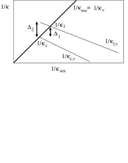
Figure 4: The values of ${1\over\kappa_{\rm V}^{c}}$ and ${1\over\kappa_{\rm V}^{\rm light}}$ are plotted versus ${1\over\kappa_{\rm sea}}$. The situation is displayed schematically around the region of the symmetric line $\kappa_{\rm sea}=\kappa_{\rm V}$.

Proceeding as in quenched simulations and measuring a bare light quark mass at each of the three sea-quark values we find light quark masses very similar to that of the quenched simulation ($5.7(4)$, $5.6(3)$, $5.4(3)$ MeV) with only a slight downward trend. An extrapolation of these quark masses in the sea-quark to the critical point would yield the value $\Delta_{2}$ in figure 4, while the true value is $\Delta_{1}$; the latter represents the value of quark masses for a physical pion in a physical sea-quark, whereas $\Delta_{2}$ is given in a sea of massless quarks. However, if we try to repair $\Delta_{2}$ by extrapolating to the light sea-quarks we have to give up working at the physical pion mass since then the critical kappa ${1\over\kappa_{\rm V}^{c}}$ is too low. This means that the light quark mass, which we wish to obtain from the physical pion mass and in a sea of physical up and down quarks, cannot be obtained by extrapolating values obtained at fixed sea-quark to either the critical or the light sea-quark mass. Figure 4 also illustrates that quenched Wilson-like light quark masses away from ${1\over\kappa_{\rm sea}^{c}}$ should be treated with caution since they lead to negative quark masses when measured with respect to the physical point ${1\over\kappa_{\rm sea}^{c}}$, $({1\over\kappa_{\rm V}^{c}}-{1\over\kappa_{\rm sea}^{c}})<0$.

Finally, we note that a study of finite size effects is under way[11]. We shall include an additional sea-quark value which will allow us to study the effects of higher order terms in chiral perturbation theory. For the simulation presented here, we postpone such a discussion to [7]. An analysis of the bottomonium spectrum, currently in progress, will allow us to use a lattice spacing obtained from the $1S-1P$ splitting, which should be less sensitive to lattice artefacts. Much more study is needed, of course, to gain control over these.
Acknowledgements
We wish to thank M. Lüscher for an interesting discussion.

References

• [1] H. Leutwyler, Phys. Lett.  B 378, 313-318 (1996); also: hep-ph/9609467, Bern preprint, September 1996.
• [2] For a recent analysis and early references, see J. Bijnens, J. Prades, and E. de Rafael, Phys. Lett. B348 (1994), 226.
• [3] B. J. Gough et al., Fermilab-Pub-96-283, hep-ph/9610223; see also the review of P.B. Mackenzie, Nucl. Phys. Proc. Suppl.53 (1997), 23.
• [4] R. Gupta and T. Bhattacharya, hep-lat/9605039, Phys. Rev.  D, to appear.
• [5] T. Bhattacharya, R. Gupta and K. Maltman, LANL preprint LA-UR-96-2698, hep-ph/9703455.
• [6] S. Güsken et al., Nucl. Phys. Proc. Suppl.17 (1990), 361.
• [7] SESAM–Collaboration, Spectrum and Decay Constants in Full QCD; in preparation.
• [8] SESAM–Collaboration, Performance of the Hybrid Monte Carlo for QCD with Wilson fermions; in preparation.
• [9] R.M. Barnett et al., Physical Review D54 (Paticle Data Booklet), 1 (1996). We use the following masses: $M_{\pi}={1\over 2}(M_{\pi^{\pm}}+M_{\pi^{0}})=137.3\;{\sf MeV}$; $M_{\rho}=769\;{\sf MeV}$; $M_{\phi}=1.019.4\;{\sf GeV}$; $M_{K}={1\over 2}(M_{K^{\pm}}+M_{K^{0}})=495.68\;{\sf MeV}$; $M_{K^{*}}=892\;{\sf MeV}$.
• [10] M. Lüscher, private communication, 24.2.97.
• [11] T$\chi$L - Collaboration, L. Conti, N. Eicker, L. Giusti, U. Glässner, S. Güsken, H. Hoeber, P. Lacock, Th. Lippert, G. Martinelli, F. Rapuano, G. Ritzenhöfer, K. Schilling, G. Siegert A. Spitz, J. Viehoff; Nucl. Phys. B 53, Proc. Suppl. (1997) 222-224 and in preparation.
• [12] G.  Martinelli and Y.  Zhang, Phys.  Lett.  B 123 (1983) 433.
• [13] G.P. Lepage and P.B.  Mackenzie, Phys.  Rev.  D48 (1993) 2250.