Scaling and confinement aspects of tadpole improved SU(2) lattice gauge theory and its abelian projection

Abstract

Using a tadpole improved SU(2) gluodynamics action, the nonabelian potential and the abelian potential after the abelian projection are computed. Rotational invariance is found restored at coarse lattices both in the nonabelian theory and in the effective abelian theory resulting from maximal abelian projection. Asymptotic scaling is tested for the SU(2) string tension. Deviation of the order of $6\%$ is found, for lattice spacings between 0.27 and 0.06 fm. Evidence for asymptotic scaling and scaling of the monopole density in maximal abelian projection is also seen, but not at coarse lattices. The scaling behavior is compared with analyses of Wilson action results, using bare and renormalized coupling schemes. Using extended monopoles, evidence is found that the gauge dependence of the abelian projection reflects short distance fluctuations, and may thus disappear at large scales.

I Introduction

Considerable progress has been achieved recently in lattice QCD as a result of combining two relatively old ideas: (I) improving the continuum limit behavior of the lattice action by adding terms that cancel the leading finite lattice spacing corrections (“Symanzik improvement” [1]) and (II) identifying a renormalized coupling which connects lattice perturbation theory and MC simulations [2, 3]. The key observation is that the disagreement between MC results and lattice perturbation theory can, to a large extent, be attributed to scale-independent (tadpole) renormalizations of the bare coupling. By converting lattice perturbation expansions in the bare coupling to ones using a renormalized coupling that effectively takes these tadpole corrections into account, lattice perturbation theory with the Wilson plaquette action can be reconciled with results from simulations in the scaling region [3]. Moreover, tests of asymptotic scaling of physical quantities are much more successful when the perturbative beta function is computed using such a renormalized coupling [4, 5, 6, 3]. At the same time, the above observation suggests a mean-field type modification of the relation between lattice links and continuum gauge fields [2, 3], which implies that the leading order coefficients of the correction terms to effect Symanzik improvement have been significantly underestimated, the more so, the coarser the lattice[7]. Thus, besides improving lattice perturbation theory, the effectiveness of lattice gluodynamics simulations per se can be dramatically enhanced by working at coarse lattices and using a tadpole improved version (henceforth referred to as “Cornell” action [7]) of the continuum limit improved action of Lüscher and Weisz [8]. The effectiveness of the method can be demonstrated, e.g., by computing the off-axis interquark potential at small $(6^{4})$, coarse lattices (lattice spacing $a\simeq 0.4$ fm) in SU(3) pure gauge theory. The violation of rotational symmetry inherent in the Wilson action, manifest in the ${\cal O}(\leq 40\%)$ deviation of the off-axis potential from a linear-plus-Coulomb fit to the on-axis values, is reduced to ${\cal O}(\leq 15\%$) using the continuum limit improved Lüscher-Weisz action, and is essentially eliminated (of order a few %) by using the continuum limit plus tadpole improved action [7].

In the present work we apply these ideas in SU(2) pure gauge theory, focusing on confinement related aspects in the framework of abelian projection (AP) picture [9, 10]. After partial gauge fixing the original SU(N) gauge symmetry is reduced to the U(1)^N-1 largest abelian (Cartan) subgroup. Under this residual group, diagonal gluon components transform as abelian “photons”, off-diagonal gluons and quarks as doubly- and singly-charged matter fields, respectively. The effective abelian theory (APQCD) that results from the integration over the off-diagonal gluons contains a complicated assortment of abelian Wilson loop operators of various sizes and charges, which describe the dynamics of the abelian photons [11, 12], and, furthermore, mass terms for monopoles of different sizes and shapes  [13]. These monopoles are identified as singularities in the gauge-fixing condition. The conjecture is then that condensation of these abelian monopoles leads to confinement, in the spirit of the dual superconductor confinement mechanism in compact QED [14, 15].

One question that we wish to address in this work is whether the improvement of the non-abelian action leads as well to improved continuum limit behavior of the effective abelian theory resulting from the projection. We do this by computing the on- and off-axis potential from abelian Wilson loops in APQCD and comparing the violation of rotational symmetry between the APQCD resulting from using the Wilson action (APQCD-W) and APQCD resulting from using the tadpole improved action (APQCD-I). We find that the off-axis abelian potential shows restoration of rotational invariance as well, allowing (at least in principle) to study the abelian projection in small, coarse lattices.

The abelian projection is gauge-dependent. Early studies [10] using local projections, e.g. diagonalizing an adjoint operator, did not seem to support ’t Hooft’s conjecture. One evidently successful projection is the maximal abelian (MA) [16, 17], corresponding in the continuum to $D_{\mu}^{n}A_{\mu}^{ch}\equiv\partial^{\mu}A^{ch}_{\mu}-ig_{0}[A^{n}_{\mu},A^{ch}_{\mu}]$ = 0, where gauge field $A$ is decomposed in neutral($n$) and charged($ch$) components, $A_{\mu}$ = $A_{\mu}^{n}$ + $A_{\mu}^{ch}$. One nice property of MA projection is that the abelian monopole density is consistent with asymptotic scaling behavior in both three [18, 19] and four [20, 21, 22] dimensional SU(2), which suggests it may be a physical quantity. However, the evidence in four dimensions is not indisputable, essentially because of the lack of a dimensionful parameter in pure gauge QCD₄. Scaling behavior has not been observed in other projections.

Thus, the second issue that we wish to address is whether renormalized perturbation theory and tadpole improvement allow to make more conclusive tests of asymptotic scaling of the monopole density. We first use renormalized perturbation theory to reanalyze the results which have been obtained with the Wilson action. In agreement with SU(3) results [3] and also with earlier SU(2) analyses [5, 6] using the “energy” scheme coupling, the asymptotic scaling behavior of the string tension shows remarkable improvement when using the “potential” scheme renormalized coupling [3]. In the case of the monopole density, however, although we do find that the degree of scaling violation is reduced when the renormalized coupling is used, asymptotic scaling is clearly violated for lattice spacings $a>0.1$ fm, independently of the coupling (bare or renormalized) used. We also find evidence for (non asymptotic) scaling of the monopole density against the string tension, which clearly breaks down for $a>0.1$ fm, as well.

We then study the string tension of the improved theory (QCD-I) and the monopole density in its abelian projection (APQCD-I). We find deviations from scaling to be typically of the same order of magnitude as with the Wilson action. Monopole properties are also similar with those in the projected Wilson theory. In particular, we see a small scaling window for the monopole density in MA gauge setting in at $\beta=3.3$ where the lattice spacing is quite small $a\simeq 0.1$ fm, and that only for relatively large lattices ($L\geq 12$). We also find good evidence for (non-asymptotic) scaling of the monopole density, although not at coarse lattices. Thus, the improvement programme reveals that the monopole definition is plagued by certain lattice artifacts that do not allow to work at coarse lattices.

A final objective of this work is to shed some light on the issue of gauge dependence of the abelian projection, along the spirit of previous work [19] in three dimensions. There, it was shown that the difference between MA and local projections can be attributed to highly-correlated short distance fluctuations. Confinement, being a large-scale phenomenon, should be oblivious to such fluctuations. It was shown that by considering monopoles defined non-locally on the lattice (extended monopoles) such fluctuations are averaged over, resulting in a converging behavior between MA and local gauges. In the last part of this work, we apply similar considerations in the four dimensional theory, using the tadpole improved action. We find a similar converging behavior of the density of extended monopoles between MA and F12 gauge as a function of the lattice size $m$ of the extended cube used to define the extended monopoles. The weakening of gauge-dependence at large physical scales is also demonstrated by showing that the density of extended monopoles in physical units forms a universal (independent of the lattice size of the extended monopole and the projection) trajectory as a function of their size in physical units. These results allow some optimism that the large-scale dynamics of the abelian projection may after all be independent of the specific gauge used to implement it.

The structure of this article is as follows: in Sec. II the action and the observables considered in this work are described. Results are presented in Sec. III and our conclusions appear in Sec. IV.

II Method

The action used in this work is a tadpole improved version of the tree-level continuum limit improved SU(2) action of Lüscher and Weisz. We begin by briefly summarizing the action improvement program. The Wilson action for SU(N) Yang Mills reads $S[U]=\beta\sum_{pl}S_{pl}$, where

$$S_{pl}\ \equiv\ {1\over N}{\rm Re{\;}Tr}(1-U_{pl})\ =\ {g_{0}^{2}\over 2N}a^{4}{\rm Tr}(F_{12}^{2})\ +\ {\cal O}(a^{6})\ .$$ (1)

Here $g_{0}^{2}=4\pi\alpha_{0}$ is the bare lattice coupling constant, $a$ the lattice spacing, and we have taken for simplicity the plaquette $U_{pl}$ to be in the (1,2) plane. The continuum action is recovered by identifying $\beta=2N/g_{0}^{2}$. To improve the continuum limit behavior of the theory (“Symanzik-improvement” [1]) one adds operators that correct for the ${\cal O}(a^{6})$ terms. Among other possible choices [23] one can use $1\times 2$ rectangular Wilson loop (labeled “$rt$”) and $1\times 1\times 1$ parallelogram Wilson loop (labeled “$pg$”) terms [8]

$$S[U]\ =\ \beta\ c_{pl}\sum_{pl}S_{pl}\ +\ \beta\ c_{rt}\sum_{rt}S_{rt}\ +\ \beta\ c_{pg}\sum_{pg}S_{pg}\ ,$$ (2)

where the sums extend over all lattice points and relevant orientations of the operators. To first nontrivial order in perturbation theory, $c_{i}=c_{i}^{0}+4\pi\alpha{}_{0}\Delta_{i}$, the action in Eq. (2) reproduces the continuum action up to and including ${\cal O}(a^{6})$ terms, provided $c_{pl}^{0}=5/3$, $c_{rt}^{0}=-1/12$, $c_{pg}^{0}=0$ (at tree level the coefficients are independent of the specific gauge group and the space-time dimensionality [24]). One loop corrections $\Delta_{i}$ have been computed by Lüscher and Weisz for both SU(2) and SU(3) (Table 1 in Ref [8]).

Following the convention of Ref. [7] we set $c_{i}\beta\rightarrow\beta_{i}$ and redefine $\beta\equiv\beta_{pl}$, which makes the tree-level coefficient of the $1\times 2$ term $-1/20$ [25]. Given $\beta$ (which implicitly determines the strong coupling) the other two couplings are perturbatively renormalized

$$\beta_{rt} = -{\beta\over 20}\biggl{[}1-\Bigl{(}{3\over 5}\Delta_{pl}+12\Delta_{rt}\Bigr{)}4\pi\alpha_{0}\biggl{]}$$ (3)

$$\beta_{pg} = {3\over 5}\beta\Delta_{pg}4\pi\alpha_{0}\ .$$ (4)

As described in Ref. [7], the continuum limit behavior of the Lüscher and Weisz action can be further improved by making the lattice links more “continuum like”. At the mean field level this entails setting $U_{\mu}\rightarrow u_{0}^{-1}U_{\mu}$, where one possible choice for the mean field factor $u_{0}$ is using the expectation value of the average plaquette

$$u_{0}=\langle{1\over N}{\rm Re{\;}Tr}U_{pl}\rangle^{1/4}\ .$$ (5)

The average plaquette with Wilson action has been calculated in lattice perturbation theory to ${\cal O}(\alpha^{2})$ [26] and recently to ${\cal O}(\alpha^{3})$ [27]. It has also been calculated using the Lüscher and Weisz action, Eq. (2), by Weisz and Wohlert [24]. However, in the latter case the result in numerically known to first order only:

$$-\log\langle{1\over N}\rm{Re{\;}Tr}U_{pl}\rangle = \xi_{N}\;\alpha{}_{s}\ ,$$ (6)

$$\xi_{N}=0.366262\;\pi{N^{2}\!-\!1\over N} = \left\{\begin{array}[]{ll}1.72597,&\mbox{for N=2}\vskip 3.0pt plus 1.0pt minus 1.0pt\\ 3.06839,&\mbox{for N=3}\end{array}\right.\ .$$ (9)

The Lüscher and Weisz action can now be tadpole improved by explicitly pulling a $u_{0}^{-1}$ factor out of each link and replacing $\alpha_{0}$ with a nonperturbatively renormalized coupling $\alpha_{s}$ defined through Eq. (6). Since $U_{pl}$ involves 4 links and $U_{rt}$, $U_{pg}$ 6 links, one further redefines $\beta\rightarrow\beta u_{0}^{-4}$, and to recover the correct continuum limit, the relative weight of the correction terms is readjusted by $u_{0}^{2}=[1-\xi_{N}\alpha{}_{s}/2]$, using Eq. (6):

$$\beta_{rt} = -{\beta\over 20u_{0}^{2}}\left[1-\left({3\over 5}\Delta_{pl}+12\Delta_{rt}+{\xi_{N}\over 8\pi}\right)4\pi\alpha_{s}\right]$$ (10)

$$\beta_{pg} = {3\over 5u_{0}^{2}}\beta\Delta_{pg}4\pi\alpha_{s}\ .$$ (11)

Using Table 1 of Ref. [8] we recover for SU(3) the improved action of Ref. [7], while for SU(2) we find

$$S=\beta\sum_{pl}S_{pl}-{\beta\over 20u_{0}^{2}}\left[1+0.2227\alpha_{s}\right]\sum_{rt}S_{rt}-0.02224{\beta\over u_{0}^{2}}\alpha_{s}\sum_{pg}S_{pg}\ .$$ (12)

The success of tadpole improvement can be seen in the value of the one-loop correction to the coefficient of the rectangular term, which for SU(2) becomes $(1.08573-0.86298)$ $\rightarrow$ $0.2227$, a quarter of the original value. This is similar to what happens in SU(3), where it was shown that the difference between results obtained using the one-loop corrected and tree-level tadpole improved actions is insignificant [7]. The results reported here are in fact obtained from simulations using tree-level improvement only, i.e.,

$$S=\beta\sum_{pl}S_{pl}-{\beta\over 20u_{0}^{2}}\sum_{rt}S_{rt}\ .$$ (13)

For recovering the correct continuum limit it is important to realize that, in the convention of Ref. [7] that we follow here, the relationship between the bare coupling $\alpha_{0}$ and the simulation parameter $\beta$ in Eq. (13) must be modified to take into account the absorption of $c^{0}_{pl}$ in $\beta$ [25]

$$\alpha_{0}={5\over 3}\ {N\over 2\pi\beta}\ ,$$ (14)

while an additional factor $(1+1.01938\ \alpha_{0})$ is needed in the case of the one-loop corrected action of Eq. (12) to account for the one-loop corrected $c_{pl}$ [23]. Arguably, the RHS of Eq. (14) should be furthermore divided by $u_{0}^{4}$. Following Ref. [23], this is not done here; instead, we will denote the coupling resulting from such a division as a “tadpole-improved” or “boosted” coupling, $\alpha_{\rm TI}=\alpha_{0}u_{0}^{-4}$, as in the case of the Wilson action.

To simulate Eq. (13) we thermalize using the heatbath algorithm, beginning with a few steps where $u_{0}$ is kept fixed to $1$. After obtaining a first estimate of the average plaquette (and therefore for $u_{0}$, cf. Eq. (5)), we thermalize a few thousand times with $u_{0}$ computed every $2-4$ updates and then fed into the action, until $u_{0}$ stabilizes within a few parts in $10^{-5}$. For extracting the on- and off-axis SU(2) potential, we compute temporal $T\times{\cal C}$ Wilson loops. Here ${\cal C}$ are spatial paths of three types: (a) straight-line spatial paths of up to 6 links, from which we extract the $R=1,2\dots 6$ on-axis potential, (b) planar spatial paths ${\cal C}=1\times 2$, $1\times 3$, from which the off-axis potential at $R=\sqrt{5},\sqrt{10}$ is extracted, and (c) cubic spatial paths ${\cal C}=1\times 1\times 1$ from which the $R=\sqrt{3}$ potential is obtained. In the case of non-straight line spatial paths we sum over the possible combinations allowed given the edges of the spatial path so as to obtain the lowest energy ($J=0$) state. Retaining only those paths minimally deviating from the diagonal, there are 2 such paths for (b) and 6 for (c). Measurements are separated by 20-100 heatbath updates.

We then perform the abelian projection to our nonabelian configurations (we henceforth restrict our attention to SU(2)). A lattice implementation of abelian projection was formulated in Refs. [10, 16], in which several gauge-fixing conditions were also developed (following ’t Hooft [9]). Local (generally nonrenormalizable) projections can be defined by the diagonalization of an adjoint operator [10]. Examples are diagonalization of a plaquette or a Polyakov line [10]. The maximal abelian (MA) projection [16] corresponds in the continuum limit to the renormalizable differential gauge $D^{3}_{\mu}A_{\mu}^{\pm}=0$, where $A^{\pm}_{\mu}\equiv(A^{1}_{\mu}\pm iA^{2}_{\mu})/\sqrt{2}$. Parametrizing the SU(2) links in the form [28, 12]

$$U_{x,\hat{\mu}}=\left(\matrix{\cos\phi_{x,\hat{\mu}}\;e^{i\theta_{x,\hat{\mu}}}&\sin\phi_{x,\hat{\mu}}\;e^{i\chi_{x,\hat{\mu}}}\cr-\sin\phi_{x,\hat{\mu}}\;e^{-i\chi_{x,\hat{\mu}}}&\cos\phi_{x,\hat{\mu}}\;e^{-i\theta_{x,\hat{\mu}}}\cr}\right)\ ,$$ (15)

with $\phi\in[0,\pi/2]$ and $\chi$, $\theta$ $\in[-\pi,\pi]$, MA projection amounts to making the transformed links $U^{\prime}_{x,\hat{\mu}}$ as close to the identity as possible

$${\rm max}\sum_{x,\mu}\cos(2\phi^{\prime}_{x,\hat{\mu}})\ .$$ (16)

Under diagonal SU(2) transformations the phases $\theta$ and $\gamma\equiv\chi+\theta$ transform like abelian gauge field and charge-two matter field (in the continuum), respectively, while $\phi$ remains invariant [12]. Eq. (16) is enforced iteratively; to speed convergence (typically by a factor of 3) we use the overrelaxation algorithm of Ref. [29] with parameter $\omega=1.7$. The iteration is repeated until the gauge transformation $G_{x}$ becomes sufficiently close to the identity at all sites

$${\rm max}\{1-{\frac{1}{2}}{\rm Tr}\,G_{x}\}\leq\delta\ll 1,$$ (17)

with $\delta={\cal O}(10^{-7})$ used as a stopping criterion.

The abelian potential after the projection is obtained from singly charged abelian Wilson loops constructed from the phases $\theta$

$$W_{T\times{\cal C}}^{abel}=\mbox{Re}\left\{\prod_{i\in{T\times{\cal C}}}e^{i\theta_{i}}\right\}=\cos\Bigl{(}\sum_{i\in{T\times{\cal C}}}\theta_{i}\Bigr{)}\equiv\cos\theta_{T\times{\cal C}}\ ,$$ (18)

with the same choice of spatial paths ${\cal C}$ as for the SU(2) Wilson loops discussed above.

Monopoles are identified in the abelian configurations using the algorithm of DeGrand and Toussaint [15]. Firstly, reduced abelian plaquette angles $\widetilde{\theta}_{pl}$ are defined

$$\widetilde{\theta}_{pl}\equiv\theta_{pl}-2\pi N_{pl},\quad\widetilde{\theta}_{pl}\in(-\pi,+\pi],$$ (19)

where $N_{pl}$ is identified with the number of Dirac strings passing through the plaquette ($N_{pl}\in\{0,\pm 1,\pm 2\}$). The net flux of monopole current out of the “elementary” (that is, of size $1^{3}$) cube $C(n,\mu)$, labeled by the dual lattice link $(n,\mu)$, is equal to the sum of Dirac strings $N_{pl}$ passing through the oriented $1\times 1$ plaquettes on the surfaces of the cube [10]

$$N_{m=1}(n,\mu)=-\sum_{pl}N_{pl}\ .$$ (20)

We also consider type-II [30] extended monopoles $N_{m}$ constructed as the number of elementary ($m=1$) monopoles minus antimonopoles in a spatial cube of size $m^{3}$. For the lattice density of monopoles we have adopted the definition of Ref. [21]

$$\rho^{[m]}_{lat}={1\over L_{t}L_{s}^{3}}\sum_{n}|N_{m}(n,4)|\ ,$$ (21)

i.e., the three-dimensional density of the time ($\mu=4$) components of the monopole currents, averaged over all time slices $L_{t}$.

III results

A The abelian potential

We first discuss the continuum limit behavior of the effective abelian theory after the projection. In Fig. 1 we show the on- and off-axis QCD potential with Wilson action (QCD-W) and the abelian potential resulting from its maximal abelian projection (MAQCD-W). The results have been obtained from 3100 configurations on a $6^{4}$ lattice at $\beta=1.7$, with measurements separated by 40-100 updates. A problem common to both Wilson and improved actions when working at coarse ($a\simeq 0.4$ fm) lattices is the difficulty in establishing plateaus in the time direction for the correlators, since after $T=2$ time slices (corresponding to 0.8 fm) the S/N ratio has dropped dramatically. In this work we follow Ref. [31] and evaluate the potential at $T=2$ [32]. The on-axis potential is fitted to an ansatz $V(r)=\sigma r-\pi/12r+c$ (dotted line). To set the scale we adopt the familiar practice [33, 6] of using the physical string tension, $a\sqrt{\sigma_{N_{c}=2,N_{f}=0}}$ = $\sqrt{\sigma_{\rm phys}}$ $\simeq 0.44$ GeV, which suggests a lattice spacing $a\simeq 0.39$ fm, corresponding to the fit value $\sigma=0.75$. The large deviation of the off-axis points from the on-axis fit shows clearly the violation of rotational symmetry plaguing both the Wilson theory and its abelian projection at coarse lattices. Results for the tadpole improved action (QCD-I) and its maximal abelian projection (MAQCD-I) are shown in Fig. 2. They come from 3200 measurements on a $6^{4}$ lattice at $\beta=2.4$. A similar fit to the potential at $T$=2 suggests $a\simeq 0.39$ fm. A more careful estimation of the string tension using APE smearing [34] shows that the lattice spacing has been overestimated by $\simeq 5\%$, and is rather close to 0.37 fm, which is, nevertheless, sufficiently coarse for our purposes. The QCD results are in agreement with recent calculations in both SU(3) [7] and SU(2) [35], and show that the continuum limit behavior of the Cornell action is clearly improved, even with tree-level tadpole improvement only.

The new feature emerging from these results is that not only QCD, but the abelian projected theory as well, shows improved continuum limit behavior and restoration of rotational invariance, at least in MA projection. In a generic (other than MA) projection, APQCD contains abelian Wilson loop operators of various sizes and charges. In order to Symanzik improve such an action, the coefficients of these terms should be carefully rearranged and, possibly, new terms should be added. It is not obvious whether the addition of the rectangular term in the QCD action with the appropriate coefficient so as to effect tree-level Symanzik improvement will, after the partial gauge fixing, automatically fine-tune the coefficients of the APQCD action in such a way as to eliminate ${\cal O}(a^{6})$ corrections in both QCD and APQCD. In the case of MAQCD-W the effective abelian action is dominated by an abelian plaquette term [11, 12, 36] and using the approximations in Ref. [36] one may argue that the observed restoration of rotational invariance is due to a corresponding improved abelian action dominating MAQCD-I. In that respect, it would be interesting to test the behavior of the off-axis abelian potential in a local projection (e.g., field-strength gauge, F12) . Although we have seen some evidence that rotational invariance is restored in F12 gauge as well, the F12 abelian Wilson loops are much more noisy and do not allow definitive conclusions to be drawn. Using anisotropic lattices may allow to clarify this point, as well as the issue of abelian dominance at small and coarse lattices, which we have not addressed here.

B scaling studies

In this section we discuss the scaling behavior of the SU(2) string tension and the abelian monopole density. The string tension has dimension [length]^-2, while (from the physical interpretation of the monopole density as defined in Eq. (21)) the monopole density has dimension [length]^-3. Thus, the monopole density in physical units reads $\rho^{[m]}$ = $\rho^{[m]}_{lat}a^{-3}$ = ${\rho^{[m]}_{lat}\over(\Lambda a)^{3}}\Lambda^{3}$, while the string tension $\sigma$ = $\sigma_{lat}a^{-2}$ = ${\sigma_{lat}\over(\Lambda a)^{2}}\Lambda^{2}$. For these quantities to be physical, the coefficient of $\Lambda^{3}$ in the monopole density that of $\Lambda^{2}$ in the string tension have to become constant (independent of $a(\beta$)) as the continuum limit is approached ($\beta\rightarrow\infty$). In previous scaling studies (with the Wilson action) the bare coupling was employed to extract a scale $\Lambda$ using the two-loop perturbative beta function

$$a(\beta)\Lambda=\left(12\pi\over 11N\alpha\right)^{51\over 121}\exp\left(-{6\pi\over 11N\alpha}\right)\ .$$ (22)

Before discussing the scaling behavior with the improved action, however, it may be instructive to revisit the scaling behavior of the Wilson action results, this time using both bare (BPT) and renormalized (RPT) perturbation theory.

1 Wilson action

In BPT, the bare coupling $\alpha_{0}$ = $(\pi\beta)^{-1}$ is used to extract the scale from Eq. (22), while, in RPT, a renormalized coupling is employed, e.g., the “energy” coupling $\alpha_{\rm E}={2N\over\pi(N^{2}\!-\!1)}(1-\langle\Box\rangle)$ [2, 4], or the “tadpole improved” coupling $\alpha_{\rm TI}=\alpha{}_{0}u_{0}^{-4}$ [3], or, more effectively, the “potential” scheme coupling $\alpha{}_{\rm V}$, defined from the nonperturbatively computed heavy-quark potential [3]. In the latter case, instead of measuring the potential, one invokes the lattice perturbation theory expansion of the heavy-quark potential [37]

$$V(q) = -{N^{2}\!-\!1\over 2N}{4\pi\alpha_{0}\over q^{2}}\left(1+\alpha_{0}\left[{N\over 3}{11\over 2\pi}\log\left(\pi\over aq\right)-{NJ\over 4\pi}\right]\right)+{\cal O}(\alpha_{0}^{3})$$ (23)

$$\equiv -{N^{2}\!-\!1\over 2N}{4\pi\alpha_{\rm V}\over q^{2}}\ ,$$ (24)

where $J=-19.695$ and $-16.954$, for $N=3$ and $N=2$, respectively, together with the analogous expansion of some other short-distance quantity, e.g., the average plaquette [26, 27],

$$1-\langle{1\over N}{\rm Re{\;}Tr}U_{pl}\rangle = c1\;\alpha_{0}+c2\;\alpha_{0}^{2}+{\cal O}(\alpha_{0}^{3})$$ (25)

$$c1={N^{2}\!-\!1\over 2N}\pi, c2=(N^{2}\!-\!1)\left({4\pi\over 2N}\right)^{2}\left(0.0203\;N^{2}-{1\over 32}\right)\ ,$$ (26)

in order to extract $\alpha{}_{\rm V}$ from the measured value of this quantity:

$$-\log\langle{1\over N}{\rm Re{\;}Tr}U_{pl}\rangle={N^{2}\!-\!1\over 2N}\pi\;\alpha_{\rm V}({q^{*}\over a})\left(1+\delta_{N}\;\alpha{}_{\rm V}\right)\ ,$$ (28)

where

$$\delta_{N}={11N\over 6\pi}\log({q^{*}\over\pi})+{NJ\over 4\pi}+{c2\over c1}+{c1\over 2}\ .$$ (29)

At $q^{*}=\pi$ one has $\delta_{N}$ = $-1.3386$ and $-0.8925$, for $N=3$ and $N=2$, respectively. According to the procedure proposed by Lepage and Mackenzie for fixing the scale, $q^{*}=3.41$ [3]. Another nonperturbative coupling may by obtained by solving Eq. (28) to first order (i.e., ignoring $\delta_{N}$) and will be denoted by $\alpha_{s}$, so as to facilitate comparisons with the improved action [cf. Eq. (6)].

Consider first the density of elementary monopoles, whose asymptotic scaling behavior has been tested, using BPT, in Refs. [20, 21]). The open circles in the inner graph of Fig. 3. correspond to the $12^{4}$ data in Fig. 1 of Ref. [20]. Although the results are not incompatible with scaling, more solid evidence is required. The recently computed three-loop beta function for Wilson action [38] modifies Eq. (22) by a factor $(1+0.08324\;4\pi\alpha_{0})$, which, however, does not improve the evidence for asymptotic scaling, since the $\beta=2.5$ and $\beta=2.6$ values come closer by less than 1%. Asymptotic scaling in MAQCD-W using the same data but renormalized perturbation theory is tested in the main graph in Fig. 3, with $a\Lambda$ extracted from the $\alpha{}_{\rm V}$ coupling and $q^{*}=3.41$. Only results with the two-loop beta function are shown, since the (scheme dependent) three-loop correction is negligible in renormalized coupling schemes [38]. The values still do not lie on a plateau, however, the $\beta$ dependence is significantly reduced: between $\beta$ = 2.5 ($a\simeq$ 0.085 fm) and 2.6 ($a\simeq$ 0.061 fm) the density drops by 23% using the bare coupling, but by much less (9%) using the potential coupling. Between $\beta$ = 2.5 and 2.7 ($a\simeq 0.045$ fm) the corresponding numbers are 37% and 13% with $\alpha_{0}$ and $\alpha_{\rm V}$, respectively. Reduced scaling violation is observed with other renormalized couplings as well, however, it is less effective compared to the potential scheme: between $\beta=2.5$ and $\beta=2.7$ we find 27% scaling violation with $a_{\rm TI}$ and 17% with $\alpha_{\rm s}$ (the “first-order potential” coupling). Results from larger lattices show smaller scaling violation: by reanalyzing the $16^{4}$ data points in Table 2 of Ref. [21] we find 9.3%, 4.5% and 4.2% scaling violation with $\alpha_{0}$, $a_{\rm TI}$ and $\alpha_{\rm s}$, respectively, between $\beta=2.5$ and $\beta=2.6$.

The information Fig. 3 reveals regarding the status of the MA monopole density as a possibly physical quantity should be properly assessed against similar tests for bona fide physical quantities, such as the string tension. Asymptotic scaling for the SU(2) string tension has been tested in bare PT [33], as well as in renormalized PT, using the energy scheme coupling [5, 6]. In Fig. 4 we reproduce the BPT test (inner graph) and also show results for RPT in the $\alpha_{\rm V}$ scheme (main graph) [39]. As has been observed in Ref. [33], asymptotic scaling is not satisfied in bare PT, although the $\beta>2.7$ data from more recent calculations [5, 6] approach a plateau. Scaling violation is substantially reduced when renormalized PT is used, in agreement with Refs. [5, 6] where the $\alpha_{\rm E}$ coupling was employed. Specifically, from Table I follows that between $a\simeq 0.17$ and $\simeq 0.4$ fm the violation of asymptotic scaling is $\simeq 27\%$ when the bare coupling is used, 16% with the tadpole improved coupling, 8% with either the energy coupling, $\alpha_{\rm E}$, or $\alpha_{\rm s}$, the coupling obtained from Eq. (28) to first order, and is reduced to 6% with the $\alpha_{\rm V}$ coupling, obtained by solving Eq. (28) to second order, with $q^{*}=3.41$.

Moreover, combining all these calculations we find behavior compatible with (non asymptotic) scaling of the monopole density against the string tension, as is seen in Fig. 5 (see also [40]). However, this scaling clearly breaks down at lattice spacings larger than some critical value somewhere between 0.12 and 0.09 fm.

2 Improved action

When testing asymptotic scaling with the improved action of Eq. (13), we again extract the scale $\Lambda$ from Eq. (22). Given the value of $\beta$ used in the simulation, several choices of associated strong couplings $\alpha$ to be used with Eq. (22) are available, as with the Wilson action, e.g., the bare coupling, Eq. (14), or the “tadpole-improved” coupling $\alpha_{\rm TI}=\alpha_{0}u_{0}^{-4}$. The situation is somehow different with respect to the potential scheme coupling, $\alpha_{\rm V}$, since, as remarked in Sec. II, the expansion leading to Eq. (6) has been (numerically) carried out to first order only. Thus, we do not have the analog of Eq. (28) whose solution (to second order) would give the corresponding $\alpha_{\rm V}$ coupling for the improved action. A solution to first order (in which case it does not matter which scale $q^{*}$ is the coupling extracted at) is available, of course, and corresponds to the nonperturbative coupling $\alpha_{\rm s}$ of Eq. (6).

Let us now discuss the results obtained with the improved action. Starting with the density of elementary $(m=1)$ monopoles in APQCD-I, results from $8^{4}$, $12^{4}$ and $16^{4}$ lattices, for $\beta$ values between 2.7 and 3.7, are shown in Fig. 6 (see also Table II). The behavior of the monopole density is very similar to what has been observed in earlier studies using the Wilson action [20, 21]. In particular, the raw density of F12 monopoles appears to be independent of $\beta$ (and therefore of the lattice spacing), implying that in physical units it diverges like $a^{-3}$. On the other hand, the MA monopoles do seem to develop an exponential falloff which is a necessary condition for scaling behavior. One also notices the considerable volume dependence of the MA monopole density results, which should be expected if monopoles play some role in the confinement mechanism: the lattice spacing is $a\simeq 0.087$ fm at $\beta=3.4$ (Table III) and the underestimation of the density on the $8^{4}$ lattices compared with the $12^{4}$ results reflects the inadequacy of the smaller lattice to provide for the typically 1 fm confinement scale (similarly at $\beta=3.5$, where $a\simeq 0.075$, between the $12^{4}$ and $16^{4}$ results). This underestimation is also in agreement with the expectation that it is the large monopole loops that are strongly correlated with confinement [41, 42].

Asymptotic scaling for the monopole density in MAQCD-I is tested in Fig. 7, using the bare coupling of Eq. (14), the boosted or tadpole-improved coupling $\alpha_{\rm TI}$, and the “first-order potential”, nonperturbative coupling $\alpha_{\rm s}$. The results are, in every case, not incompatible with scaling, at level similar to that of the Wilson action results: between $\beta$ = 3.4 and 3.6 ($a\simeq 0.087$ and 0.063 fm, respectively, corresponding roughly to the $\beta\in[2.5,2.6]$ interval for the Wilson action discussed above) the scaling violation of the $16^{4}$ data is 8.6%, 6.1% and 3.4% using $\alpha_{0}$, $\alpha_{\rm TI}$ and $\alpha_{\rm s}$, respectively. At even smaller lattice spacings, for fixed lattice size, the lattice volume becomes too small and this results in the expected “enveloping” curve [20].

Turning to the string tension, this is extract from linear + Coulomb chi-squared fits (without fixing the Coulomb coefficient to the Lüscher value) to the time-dependent potential $V(R,T)$ = $\log\left(W[R,T\!-\!1]/W[R,T]\right)$, using jackknife errors for $V(R,T)$. It is known that the correction terms in the action spoil the hermiticity of the transfer matrix [43]. As a result, correlators show damped oscillatory behavior in $T$ [32]. Using APE smearing [34], we have nevertheless established plateaus in $T$ in our fits of the string tension (Table III); results from the $16^{4}$ lattices are shown in in Table IV. Above $\beta=3.4$ the string tension from $12^{4}$ lattices (not shown in Table IV) is underestimated (commensurate with the deviation of the monopole density results between $12^{4}$ and $16^{4}$ lattices discussed above), since the lattice size is below 1 fm in this case. This can be seen in Fig. 8, where we test asymptotic scaling for the string tension using the improved action, and with the same choice of couplings as for the monopole density. Since the three-loop correction to the beta function is not universal, the Wilson action computation in Ref. [38] in not applicable in this case. The results appear compatible with asymptotic scaling, especially when the boosted coupling, $\alpha_{\rm TI}$, is used. Specifically, from Table V is seen that the violation of asymptotic scaling between $\beta=2.7$ ($a\simeq 0.26$ fm) and $\beta=3.6$ ($a\simeq 0.06$ fm) is $\simeq 6\%$ with $\alpha_{\rm TI}$, but more pronounced, $\simeq$ 12.5%, using either one of $\alpha_{\rm 0}$, $\alpha_{\rm s}$ and $\alpha_{\rm E}=(1-\langle\Box\rangle)/1.7259$ (not shown). Apparently (and unlike the monopole density results discussed above) the nonperturbative coupling $\alpha_{\rm s}$ is not so successful here, compared to $\alpha_{\rm TI}$. However, this depends strongly on the value of the string tension at the coarser lattice considered, $\beta=2.7$: the scaling violation between $\beta=2.9$ ($a\simeq 0.2$ fm) and $\beta=3.6$ is 6% and 4% with $\alpha_{\rm TI}$ and $\alpha_{\rm s}$, respectively. In general, asymptotic scaling tests using these two couplings give rather similar results, since the ratio $\alpha_{\rm s}/\alpha_{\rm TI}$ slowly varies around 0.930 with either Wilson or improved action, as seen from Tables I and V. Notice, though, that the ratio does not monotonically decrease with $\beta$, as does, e.g., for the ratio $\alpha_{\rm s}/\alpha_{0}$ in the case of the improved action [cf. Table V], or, in the case of the Wilson action, when one instead of using $\alpha_{\rm s}$ solves Eq. (28) to second order to obtain $\alpha_{\rm V}$ (last column in Table I). It is conceivable that knowledge of the second order terms in Eq. (6) and the improved action lattice perturbation expansion of the potential (the analog of Eq. (23)), which would allow to extract the $\alpha_{\rm V}$ coupling with the improved action, might lead to even smaller asymptotic scaling violation.

As with the Wilson action, we can now combine the results to test (non asymptotic) scaling. Reading off $\sqrt{\sigma}\simeq 3.8\Lambda_{\rm TI}$ from Fig. 8(b) and estimating the scaling value for the monopole density at $\rho^{[1]}\simeq$ 54$\Lambda_{\rm TI}^{3}$ from Fig. 7(b) suggests that the dimensionless combination $\rho^{[1]}\sigma^{-3/2}$ should saturate to $54\times 3.8^{-3}\simeq 1$. This is indeed verified in Fig. 9. By combining the $12^{4}$ and $16^{4}$ results for the two quantities, their individual volume dependence cancels, to a large extent, in the dimensionless ratio. Thus, the evidence for scaling from this graph is more compelling than the evidence for asymptotic scaling in Fig. 7. It appears, therefore, that the elementary monopole density in maximal abelian gauge is indeed a physical quantity. Using $\sqrt{\sigma}=0.44$ GeV with $\rho^{[1]}\simeq\sigma^{3/2}$ implies a density of approximately 11 elementary monopoles per fm³, in good agreement with estimates using the Wilson action [21]. However, although scaling is observed, its onset is at relatively small lattice spacings $a\simeq$ 0.1 fm, and therefore the situation for the monopole density is quite similar to what we found with the Wilson action (Fig. 5).

3 Comparison of Wilson and improved action

A comparison of the scaling results discussed above with the two actions suggests the following:

1. In both cases, renormalized couplings lead to improved asymptotic scaling behavior compared to the bare coupling; among renormalized couplings, the nonperturbative ones ($\alpha_{\rm s}$ or $\alpha_{\rm V}$, when available) are typically more successful than the tadpole-improved coupling $\alpha_{\rm TI}$.

2. The string tension using the Wilson action shows more pronounced scaling violation compared to using the improved action, but only when analyzed with the bare coupling. When renormalized couplings are used, the results are rather similar for the two actions, for both observables tested here (string tension and monopole density), i.e., renormalized PT with the improved action does not improve renormalized PT analyses of Wilson action results significantly. Thus, the results using the improved action lead to the same interpretation as the one drawn from using a renormalized coupling with the Wilson action:

   • the string tension calculation suggests that the improvement program does allow confinement to be studied at relatively coarse lattices.

   • evidently a physical quantity, the monopole density in maximal abelian projection is, nevertheless, sensitive to small distance ($a=0.1$ fm) physics. This sensitivity persists even when a continuum limit improved action is used.

   In that respect, the merit of the tadpole-improvement program (in the form of, first, renormalized perturbation theory, and second, tadpole-improving the action itself), insofar as abelian monopoles are concerned, has been to point out that the asymptotic scaling behavior of the string tension can be extended to coarser lattices, while that of the monopole density can not, something that — due to the lack of asymptotic scaling with Wilson action and with the bare coupling — could not have been previously realized. To further clarify some of the above points, more accurate determinations of the string tension with the improved action using anisotropic lattices (following Ref. [32]) and, possibly, a continuum limit improved version of Creutz ratios, should be performed [44].

C Gauge dependence and extended monopoles

It has been pointed out by several authors [19, 20, 21, 22, 28] that the large number of monopoles and the associated scaling violation observed in local, unitary gauges (such as F12 or Polyakov gauge) can, to some degree, be attributed to strong short distance fluctuations. Defining monopoles nonlocally (e.g., extended monopoles, introduced first by Ivanenko et al. [30]), may help average –at least partially– over such fluctuations and therefore reduce the gauge-dependence of the abelian projection. The main results of an analysis along these lines in the $d=3$ theory with Wilson action by Trottier, Woloshyn and this author were the following [19]:

1. monopoles in MA projection form a dilute plasma in $d=3$. The monopole distribution is basically random and characterized by the average minimum monopole-antimonopole separation $\langle r_{\rm min}\rangle$ which in physical units scales. The density of extended monopoles $\rho^{[m]}_{lat}$ remains roughly the same for “sizes” $ma<\langle r_{\rm min}\rangle$ (in physical units).

2. In local gauges $\rho^{[1]}_{lat}$ does not scale. The distribution is significantly narrower than what expected from a random distribution, indicating strong short-distance correlations. However, unlike MA monopoles, $\rho^{[m]}_{lat}$ drops rapidly with $m$, suggesting that by considering extended monopoles such correlations (which are absent in MA projection but create “spurious” monopoles in, e.g., F12) are being “washed out”. Accordingly, the ratio of extended monopoles between F12 and MA projections is found to decrease as $m$ increases.

3. For extended monopoles with fixed (physical) size, $\rho^{[m]}$ (in physical units) scales for MA gauge but not for local ones. However, the degree of scaling violation is found to decrease substantially as the extended monopole size increases.

To what extent do such considerations apply to the four-dimensional theory? The situation appears quite similar on a first inspection: $\rho^{[m]}_{lat}$ drops faster in the local projections than in MA, as can be seen by plotting the ratio $R^{[m]}\equiv$ $\rho^{[m]}_{F12}/\rho^{[m]}_{MA}$ as a function of $m$ (Fig. 10). Empirically, we find that the extended monopole density in local gauges (which is, in $d=4$, practically independent of the lattice spacing for all $m$) behaves like

$$\rho^{[m]}_{lat}(\beta)={C\over m^{\gamma}}\ ,$$ (30)

with $C=0.31(1)$ and $\gamma=1.64(1)$, over a range of $\beta$ values where the lattice spacing drops by a factor of 3 (Fig. 11); $C$ and $\gamma$ depend very mildly on the particular local gauge fixing, suggesting a purely geometrical origin of $\gamma$, which, however, we have not identified. The MA density can also be parametrized in the form of Eq. (30), although the fits are not equally good. In this case the the coefficients decrease with $\beta$, mildly for $\gamma_{\rm MA}$ (Fig. 11) and exponentially for $C_{\rm MA}$ (not shown). Since $\gamma_{\rm MA}<\gamma_{\rm F12}$, the convergence between $\rho^{[m]}_{\rm MA}$ and $\rho^{[m]}_{\rm F12}$ for fixed $\beta$ seen in Fig. 10 readily follows from this parametrization. The more rapid convergence for the higher $\beta$ values observed in Fig. 10 is accounted for by $\gamma_{\rm F12}$ and $\gamma_{\rm MA}$ being independent of $\beta$ and decreasing with $\beta$, respectively.

Moreover, one may show that, although, as in $d=3$, $\rho^{[m]}=Cm^{-\gamma}a^{-3}$ (the density in physical units) does not scale, the degree of scaling violation decreases as a function of the monopole size $ma$ in physical units. Unlike $d=3$, where $\beta$ is dimensionful and therefore this can be tested directly by comparing densities with $m/\beta$ = fixed, in $d=4$ can only be implicitly deduced, from Eq. (30); indeed, a measure of scaling violation, as the continuum limit $a\rightarrow 0$ is approached, is given by $\partial\rho^{[m]}/\partial a^{\epsilon}$, with $\epsilon<0$. From the above parametrization

$$\left.{\partial\rho^{[m]}\over\partial a^{\epsilon}}\right|\begin{array}[]{ll}\\ {}_{{ma}={\rm fixed}}\end{array}=C(ma)^{-\gamma}\ ,\epsilon=\gamma-3<0\ \ .$$ (31)

Since $0<\gamma<3$, the degree of scaling violation for the extended monopole density in unitary gauges will decrease as a function of the extended monopole size (in physical units), like in QCD₃ [19].

These results suggest that there is more contamination from short-distance physics in the local projection, as expected from the non-locality of the gauge condition in maximal abelian projection. In attempting to draw parallelisms with the $d=3$ case, one should bear in mind that monopole d.o.f. are pointlike in $d=3$ but form closed loops in $d=4$. Thus, although a concept of minimum separation can still be devised at $d=4$, it is probably not the correct way to describe the monopole distribution. Indeed, although we find that $\langle r_{\rm min}\rangle$ is larger in MA than in F12 projection (by a factor ranging from 1.2 to 2 for the $\beta$ values we have considered), when converted to physical units neither scales. That may explain why $\rho^{[m]}_{lat}$ in MA projection does not remain constant over some range in Fig 10, as in $d=3$, but instead starts to drop immediately with increasing $m$. The appropriate way to describe the monopole distribution is probably by categorizing the loops according to their length [42]; although not discussed here, the analog of the $d=3$ case may be to examine how close to random the MA monopole loop length distribution found in Ref. [42] is.

In order to test the behavior of monopoles at large scales we plot in Fig. 12 a family of $m={\rm fixed}$ trajectories for $\rho^{[m]}_{\rm F12}$ and $\rho^{[m]}_{\rm MA}$ as functions of the extended monopole size $ma$ in physical units, using the scale extracted from the $\alpha_{\rm TI}$ coupling. The linear behavior of the F12 data points, with the $m$-independent, equal to $-3$, slope and the increasing like $\log m$ ordinates for a given abscissa, follows directly from the $\beta$-independence of the coefficients in Eq. (30) with $\gamma<3$:

$$\log\left(\rho^{[m]}_{lat}a^{-3}\right)=\log C+(3-\gamma)\log m-3\log\left(ma\right)\ .$$ (32)

For each individual $m=\rm{fixed}$ trajectory, Fig. 12 essentially tests asymptotic scaling for $\rho^{[m]}$. The most interesting feature is the formation of a universal, i.e., $m$-independent, trajectory for MA extended monopoles of large size in physical units. Unlike the F12 case, the dependence of $C_{\rm MA}$, $\gamma_{\rm MA}$ on $\beta$ (and therefore, implicitly, on $a$) does not allow a simple explanation of this feature. The deviation of the individual $m={\rm fixed}$ curves from this universal trajectory occurs at $ma_{c}\Lambda_{\rm TI}\simeq$ 0.32 , 0.22, 0.16, 0.11, for $m=$ 6, 4, 3, 2, respectively. Thus, the crossover points involve a common critical lattice spacing $a_{c}\Lambda_{\rm TI}\simeq 0.055$, which, from the scaling value $\sqrt{\sigma}$ = 3.8$\Lambda_{\rm TI}$ = 0.44 GeV implies $a_{c}\simeq 0.094$ fm. Given that these results are from $12^{4}$ lattices, and since for fixed $m$ the continuum limit is to the left on the horizontal axis in Fig. 12, it appears that this deviation from the universal trajectory is merely another manifestation of the finite physical volume effect occurring when the lattice size $La$ is less than 1 fm, as described in [20] and also observed in Sec. III. It is quite conceivable that towards the infinite volume limit this universal trajectory will extend to arbitrarily small physical sizes. We also notice that the difference between MA and F12 results decreases rapidly with increasing monopole size and at large physical sizes a projection-independent trajectory seems to form, indicating that also in $d=4$ the abelian projection shows evidence of gauge independence when large scales in physical units are probed.

IV summary

In this work the ideas of renormalized perturbation theory and tadpole improvement have been used to study confinement related aspects of lattice SU(2) gluodynamics. Observables have been studied that are either directly related to confinement, e.g., interquark potential/string tension, or conjectured to be in the context of a dual superconductor picture, e.g., monopoles and abelian potential after the abelian projection. Two types of studies have been undertaken. Firstly, tests of the improvement program in QCD and its abelian projection, APQCD, specifically (a) whether asymptotic scaling and scaling is observed, and (b) what is the continuum limit behavior of APQCD at small, coarse lattices. Secondly, studies of extended monopoles, using the tadpole improved action as a new, better tool, with the objective of shedding some light onto the issue of the apparent, albeit bothersome, gauge dependence of the abelian projection. The results can be summarized as follows:

• At small, coarse lattices the degree of violation of rotational invariance is similar in Wilson QCD and its abelian projection. With the improved action, though, rotational invariance is restored in both QCD and the corresponding abelian theory, at least in MA projection.

• Deviation from asymptotic scaling for the SU(2) string tension is observed at the 6% level between $a=0.06$ and 0.26 fm. This order of scaling violation is quite similar with renormalized coupling analyses of Wilson action results, although considerably improved in comparison to the corresponding bare coupling analysis, even when the three-loop beta function is used. The quality of our calculation does not allow statements to be made about scaling at the 1% level. Using anisotropic lattices, will allow more accurate determination of the string tension for lattice spacings $a>0.2$ fm. However, it does not seem very likely that, even with this technique, asymptotic scaling will be verified at the 1% level for coarse and small lattices. The fact that continuum limit improvement is not very evident in the string tension calculation, is, however, not surprising, since the string tension is obtained from the standard on-axis potential.

• Good evidence for scaling of the density of maximal abelian monopoles (using the SU(2) string tension to set the scale) is found. Some evidence for asymptotic scaling is seen as well, although hampered by finite volume effects. It is, nevertheless, clear, that neither scaling nor asymptotic scaling hold for the MA monopole density at as coarse lattices as 10% asymptotic scaling for the string tension does.

• The gauge dependence of the density of abelian monopoles is significantly reduced when considering extended monopoles of large sizes in physical units.

The scaling studies of the monopole density suggest that the monopole density in MA projection is a physical quantity, and thus seem to settle a hitherto not entirely clarified issue. Together with the reduced scaling violation in local projections at large scales, this may be considered as supporting evidence for the abelian projection picture of confinement. However, despite the encouraging results from the off-axis abelian potential, scaling of the monopole density breaks down at coarse lattices. It is conceivable that this necessitates improvement of the monopole identification algorithm besides improving the action [45].

TABLE I.: Asymptotic scaling test for SU(2) string tension with Wilson action. Different coupling schemes are used to get $a(\beta)\Lambda$ from Eq. (22). The bare coupling $\alpha_{0}=(\pi\beta)^{-1}$, the tadpole improved coupling $\alpha_{\rm TI}=\alpha_{0}\langle\Box\rangle^{-1}$, the energy coupling $\alpha_{\rm E}={4\over 3\pi}(1-\langle\Box\rangle)$, and the potential coupling obtained from Eq. (28) with $q^{*}=3.41$, to first order, $\alpha_{s}=-{4\over 3\pi}\log\langle\Box\rangle$, and to second order, $\alpha_{\rm V}$. Data from [5, 6] and references therein.

$\beta$	$<\Box>$	$\sqrt{\sigma}$	$\sqrt{\sigma}\over\Lambda_{0}$	$\sqrt{\sigma}\over\Lambda_{\rm TI}$	$\sqrt{\sigma}\over\Lambda_{\rm E}$	$\sqrt{\sigma}\over\Lambda_{s}$	$\sqrt{\sigma}\over\Lambda_{\rm V}$	$\alpha_{s}\over\alpha_{\rm TI}$	$\alpha_{\rm V}\over\alpha_{\rm TI}$
2.3	0.6024	0.3690(30)	62.4( 5)	6.59( 5)	22.29(18)	2.49(2)	1.12(1)	0.936	1.199
2.4	0.6300	0.2660(20)	57.8( 4)	6.44( 5)	22.75(17)	2.55(2)	1.16(1)	0.931	1.155
2.5	0.6522	0.1870(10)	52.3( 3)	6.03( 3)	22.07(12)	2.47(1)	1.14(1)	0.929	1.127
2.5115	0.6544	0.1836(13)	52.9( 4)	6.11( 4)	22.41(16)	2.51(2)	1.15(1)	0.929	1.124
2.6	0.6701	0.1360(40)	49.0(14)	5.76(17)	21.52(63)	2.41(7)	1.11(3)	0.930	1.109
2.635	0.6757	0.1208( 1)	47.5( 1)	5.62( 1)	21.08( 2)	2.36(1)	1.09(1)	0.931	1.104
2.7	0.6856	0.1015(10)	47.1( 5)	5.62( 6)	21.28(21)	2.38(2)	1.11(1)	0.932	1.096
2.74	0.6913	0.0911( 2)	46.8( 1)	5.61( 1)	21.32( 5)	2.38(1)	1.11(1)	0.932	1.092

TABLE II.: Runs for monopole density determination. After $N_{\rm therm}$ thermalization steps, $N_{\rm measur}$ measurements are taken, separated by $N_{\rm separ}$ updates.

$\beta$	lattice	$N_{\rm therm}$	$N_{\rm measur}$	$N_{\rm separ}$	$<\Box>$	$\rho^{[1]}_{\rm MA}$
2.7	$12^{4}$	$-$	100	100	0.5771(2)	0.09157(27)
2.9	$12^{4}$	2500	500	60	0.6216(1)	0.05295(10)
3.1	$12^{4}$	2500	500	60	0.6581(1)	0.02548( 9)
3.2	$12^{4}$	$-$	30	20	$-$	0.01641(36)
	$16^{4}$	2500	30	50	0.6730(1)	0.01706(13)
3.3	$12^{4}$	2500	500	60	0.6862(1)	0.01106( 7)
	$16^{4}$	3000	30	50	0.6864(1)	0.01068(17)
3.4	$12^{4}$	3000	30	70	0.6980(2)	0.00662(29)
	$16^{4}$	2500	30	60	0.6979(1)	0.00724(13)
3.5	$12^{4}$	2500	50	100	0.7086(2)	0.00364(22)
	$16^{4}$	2500	100	50	0.7086(1)	0.00450( 8)
3.6	$12^{4}$	3000	30	70	0.7182(2)	0.00164(14)
	$16^{4}$	$-$	26	$-$	$-$	0.00271(21)

TABLE III.: String tension $\sigma_{T}$ and the corresponding lattice spacing, as extracted from linear-plus-Coulomb fits to $V(R,T={\rm fixed})$.

$\beta$	$T$	$\sigma_{T}$	$\sigma_{T+1}$	a (fm)
3.1	3	0.0985( 8)	0.0965(13)	0.141( 6)
3.3	4	0.0483(11)	0.0476(16)	0.098(11)
3.4	5	0.0378( 9)	0.0377( 7)	0.087(11)
3.5	5	0.0278( 6)	0.0277( 7)	0.075( 8)

TABLE IV.: Runs for string tension determination. $N_{\rm iter}$ iterations of APE smearing with parameter $c_{0}$ are used.

$\beta$	lattice	$N_{\rm therm}$	$N_{\rm measur}$	$N_{\rm separ}$	$c_{0}$	$N_{\rm iter}$	$<\Box>$	$\sigma$
3.1	$16^{4}$	2500	200	40	8	20	0.6581(1)	0.0985(20)
3.2	$16^{4}$	2500	200	40	6	20	0.6732(1)	0.0702(20)
3.3	$16^{4}$	2500	200	20	6	20	0.6862(1)	0.0483(19)
3.4	$16^{4}$	2500	200	20	5	20	0.6980(1)	0.0378( 5)
3.5	$16^{4}$	2000	200	20	5	20	0.7086(1)	0.0278( 7)
3.6	$16^{4}$	$-$	200	20	5	20	0.7184(1)	0.0195(10)

TABLE V.: Asymptotic scaling for SU(2) string tension with improved action. Different coupling schemes are used to get $a(\beta)\Lambda$ from Eq. (22): $\alpha_{0}={5\over 3}(\pi\beta)^{-1}$, $\alpha_{\rm TI}=\alpha_{0}\langle\Box\rangle^{-1}$, and $\alpha_{s}=-{\log\langle\Box\rangle\over 1.726}$, from Eq. (6).

$\beta$	lattice	$\sqrt{\sigma}\over\Lambda_{0}$	$\sqrt{\sigma}\over\Lambda_{\rm TI}$	$\sqrt{\sigma}\over\Lambda_{\rm s}$	$\alpha_{s}\over\alpha_{0}$	$\alpha_{s}\over\alpha_{\rm TI}$
2.7	$12^{4}$	18.86(52)	3.76(10)	4.35(12)	1.732	0.935
2.9	$12^{4}$	18.84(47)	3.91(10)	4.64(12)	1.609	0.936
3.1	$16^{4}$	17.75(18)	3.82( 4)	4.72( 5)	1.519	0.932
3.2	$16^{4}$	17.38(25)	3.79( 5)	4.76( 7)	1.486	0.931
3.3	$16^{4}$	16.73(33)	3.68( 7)	4.68( 9)	1.457	0.931
3.4	$16^{4}$	17.17(11)	3.81( 3)	4.89( 3)	1.433	0.932
3.5	$16^{4}$	17.10(22)	3.81( 5)	4.93( 6)	1.411	0.933
3.6	$16^{4}$	16.63(43)	3.72(10)	4.85(12)	1.392	0.934

FIG. 1.: The on-($\Box$) and off-axis ( ) nonabelian (a) and abelian (b) potential, from $6^{4}$ lattices at $\beta=1.7$, using the Wilson action.

FIG. 2.: As in Fig. 1 but using the improved action, at $\beta=2.4$, where the lattice spacing is approximately the same.

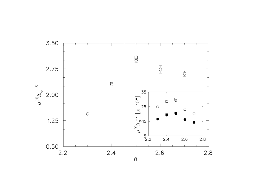
FIG. 3.: Asymptotic scaling test for the density of elementary monopoles in MA projection using the Wilson action (MAQCD-W). Data from Ref. [20] (circles) and Ref. [21] (squares). Open symbols: 2-loop evolution with the $\alpha_{\rm V}$ coupling [Eq. (28)] for the main graph, and the bare coupling $\alpha_{0}$ = $(\pi\beta)^{-1}$ for the inner graph. Solid symbols: 3-loop evolution (bare coupling only). The dashed line corresponds to the scaling curve, $\rho=[66\Lambda]^{3}$, quoted from Ref. [20].

FIG. 4.: Asymptotic scaling test for the Wilson action SU(2) string tension. The scale $a\Lambda$ is extracted as in Fig. 3. Data from Refs. [5, 6, 33].

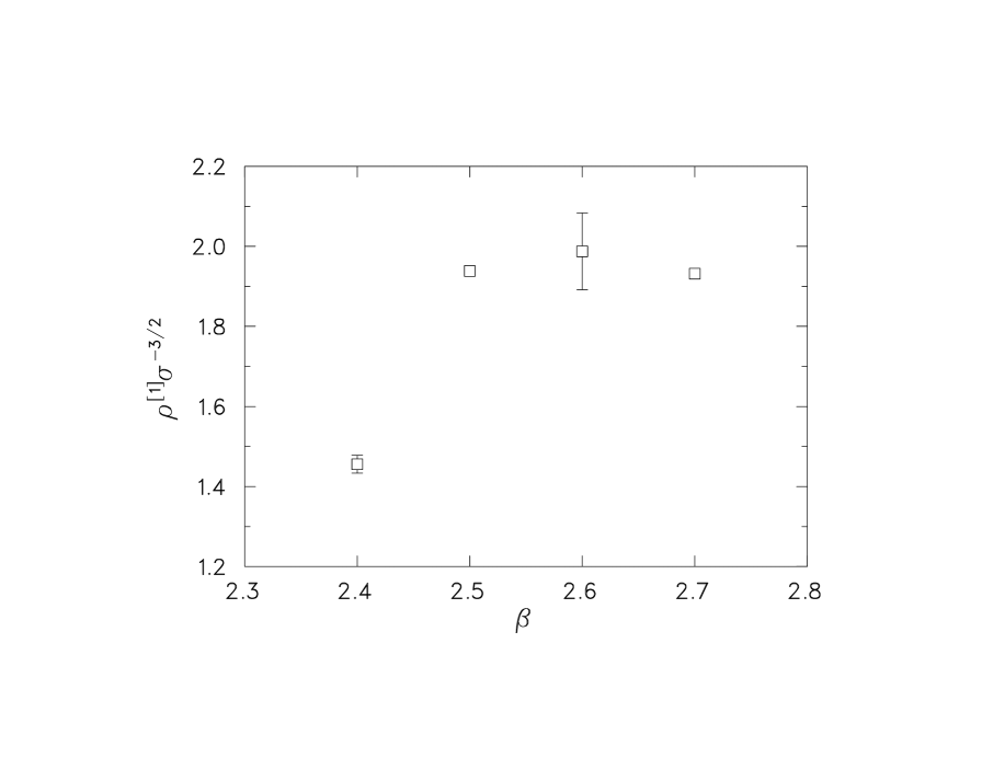
FIG. 5.: Scaling test for the density of elementary monopoles against the nonabelian string tension, using the Wilson action. Data from Refs. [5, 20, 33].

FIG. 6.: The density of elementary monopoles (in lattice units) in the abelian-projected improved theory (APQCD-I). Results shown for F12 projection on $8^{4}$ lattices ($\Diamond$), and MA projection on $8^{4}$ ($\triangle$), $12^{4}$ (o) and $16^{4}$ ($\Box$) lattices.

FIG. 7.: Asymptotic scaling test for the density of elementary monopoles in maximal abelian projected SU(2) using the improved action (MAQCD-I). The scale $a\Lambda$ is extracted (a) from the bare coupling $\alpha_{0}$ [Eq. (14)], (b) from the boosted coupling $\alpha_{\rm TI}=\alpha_{0}u_{0}^{-4}$, and (c) the nonperturbative coupling $\alpha_{\rm s}$ [Eq. (6)]. Results shown for $12^{4}$ (o) and $16^{4}$ ($\Box$) lattices.

FIG. 8.: Asymptotic scaling test for the nonabelian string tension with improved action (QCD-I). The scale is extracted as in Fig. 7. Results are shown for $12^{4}$ (o) and $16^{4}$ ($\Box$) lattices. The dashed line in (b) corresponds to $3.8\Lambda_{\rm TI}$.

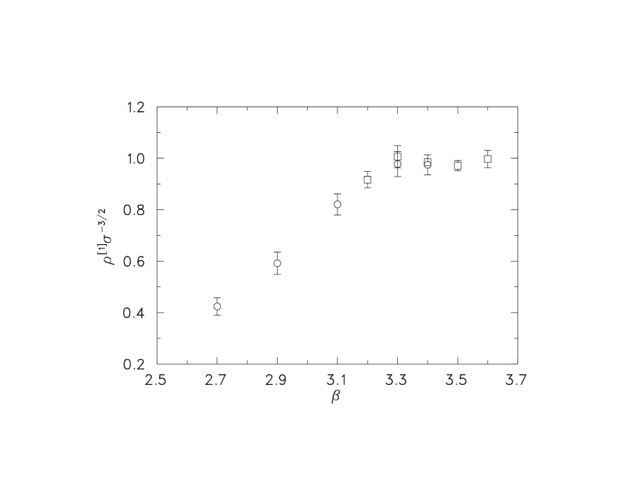
FIG. 9.: Scaling test for the density of elementary monopoles against the nonabelian string tension, using the tadpole improved action. Results are shown for $12^{4}$ (o) and $16^{4}$ ($\Box$) lattices.

FIG. 10.: The ratio of densities of extended monopoles between F12 and MA projections using the improved action, as function of the size $m$ of the lattice cube defining the type-II extended monopole. Results from $12^{4}$ lattices at $\beta$ = 2.7 ($\Box$), $\beta$ = 3.1 ($\Diamond$), $\beta$ = 3.3 (o), $\beta$ = 3.5 ($\triangle$),

FIG. 11.: Fitting the lattice density of type-II extended monopoles according to Eq. (30): $C_{\rm F12}$ (o), $\gamma_{\rm F12}$ ($\Box$), $\gamma_{\rm MA}$ ( ). Dashed line corresponds to $C$=0.31 and dotted line to $\gamma$=1.64 (see text).

FIG. 12.: The density of extended monopoles as a function of their size for F12 and MA projections.