Complete ${\mathcal{O}}(v^{2})$ corrections to the static interquark potential from SU(3) gauge theory

Abstract

For the first time, we determine the complete spin- and momentum-dependent order $v^{2}$ corrections to the static interquark potential from simulations of QCD in the valence quark approximation at inverse lattice spacings of 2–3 GeV. A new flavor dependent correction to the central potential is found. We report a $r^{-2}$ contribution to the long range spin-orbit potential $V_{1}^{\prime}$. The other spin-dependent potentials turn out to be short ranged and can be well understood by means of perturbation theory. The momentum-dependent potentials qualitatively agree with minimal area law expectations. In view of spectrum calculations, we discuss the matching of the effective nonrelativistic theory to QCD as well as renormalization of lattice results. In a first survey of the resulting bottomonia and charmonia spectra we reproduce the experimental levels within average errors of $12.5$ MeV and $22$ MeV, respectively.

I Introduction

Quarkonia spectroscopy provides a wealth of information and thus constitutes an important observational window to the phenomenology of confining quark interactions. It has been known for a long time that purely phenomenological or QCD inspired potential models offer a suitable heuristic framework to understand the empirical charmonium ($J/\psi$) and bottomonium ($\Upsilon$) spectra [1, 2, 3, 4].

On a more fundamental level, one would prefer to start out from the basic QCD Lagrangian to solve the heavy quarkonia bound state problem. NRQCD [5] offers a systematic way to solve this problem by direct extraction of bound state masses from effective nonrelativistic lattice Lagrangians, which approximate the QCD Lagrangian to a given order in the quark velocity, $v$. Considerable success has been achieved recently in determining quarkonia spectra within this approximation to QCD [6].

Here, we follow a complementary strategy: instead of separately computing the spectral properties of individual mesonic states, we integrate out the gauge background and directly determine the underlying quantum mechanical two-particle Hamiltonian. Once QCD binding problems are recast into this form, spectra, wave functions and decay constants for arbitrary (sufficiently large) quark masses and quantum numbers can easily be obtained. Results can either be confronted with experiment or compared to predictions from lattice NRQCD.

In the limit of infinite quark mass, the Born-Oppenheimer approximation is applicable and, after integrating out the gauge degrees of freedom, QCD binding problems become nonrelativistic. The static interaction potential can be computed directly from the QCD Lagrangian on the lattice. Within the present study, we find the average velocity between the sources to be $\langle v^{2}\rangle\approx 0.27$ and $\langle v^{2}\rangle\approx 0.08$ for the charmonium and bottomonium ground-states, respectively. This leads us to expect that the phenomenological potentials within those models, which have been optimized to reproduce empirical spectra, should deviate by substantial ${\mathcal{O}}(v^{2})$ corrections from the static potential as predicted by QCD; at realistic quark masses such corrections, that are also required to obtain hyperfine splittings, cannot be neglected. Therefore, we have to take corrections to the static limit into account.

The Hamiltonian that we derive is equivalent to the QCD Lagrangian up to ${\mathcal{O}}(v^{2})$. It includes the spin-dependent (SD) terms derived by Eichten, Feinberg and Gromes [7, 8], the momentum-dependent (MD) corrections derived by Barchielli, Brambilla, Montaldi and Prosperi (BBMP) [9] and one-loop radiative corrections from matching the effective theory to the full theory at a scale $\mu$ that, in general, differs from the heavy quark mass, $m$ [10]. It can be parametrized in terms of seven independent scalar functions of the quark separation (the potentials). These will be computed nonperturbatively on the lattice.

The static potential has been determined with high accuracy in the valence quark (quenched) approximation to QCD [11, 12, 13] and, more recently, in full QCD with two dynamical flavors of light Wilson sea quarks [14]. First attempts to compute relativistic corrections have been made in the mid eighties for SU(2) and SU(3) gauge theory [15, 16, 17, 18] and have been extended to QCD with sea quarks in Refs. [19, 20].

In view of the general interest in the Hamiltonian formulation of the meson binding problem, renewed effort should be made to unravel the structure of the SD potentials and other ${\mathcal{O}}(v^{2})$ corrections. Recently, we presented improved techniques for computation of SD corrections and tested them successfully on SU(2) gauge theory [21]. Here, we shall apply these methods to the physically relevant SU(3) gauge theory. We will extend the SU(2) investigation by inclusion of MD potentials and relativistic corrections to the central potential, and subsequently determine quarkonia levels.

We wish to emphasize that the method presented does not rely on any other approximations than truncating the QCD Lagrangian at second order in the quark velocity (apart from the valence quark approximation). However, the Schrödinger-Pauli approach to heavy quark binding problems suffers from the same difficulties as NRQCD, namely (a) the error involved in truncating the expansion at a finite order in $v$, (b) uncertainties in the matching of the effective Hamiltonian to QCD and (c) renormalization of lattice results. While we manage to solve the latter problem in a satisfactory way, we have to rely on one-loop perturbation theory for the matching of the nonrelativistic Hamiltonian to QCD. Systematic errors from the ${\mathcal{O}}(v^{2})$ approximation as well as from the uncertainty in the matching constants (that can be reduced order by order in perturbation theory) are estimated.

Since NRQCD to order $v^{2}$ (or $v^{4}$, depending on the labeling conventions used) is based on the same Lagrangian, it is worthwhile to compare the two approaches. While NRQCD can in principle be generalized to any order in $v$, the Schrödinger-Pauli approach is only valid up to order $v^{2}$. Also, we cannot treat heavy-light systems. In NRQCD the zero point energy can be fixed by measuring the dispersion relation while in our approach only properties of particles at rest can be studied. The clear advantage of the method presented here is that with one simulation only, we easily obtain all spectral properties (including arbitrary excitations) for any (sufficiently heavy) quark mass. From a two-body Hamiltonian formulation of the problem, the effect of individual terms on the spectrum becomes immediately apparent, and a transparent understanding of the anatomy of the underlying interaction mechanism is obtained. The potentials are protected by the global $Z_{3}$ symmetry [22] from finite size effects, contrary to NRQCD wave functions and masses, such that we can determine the potentials for the $r$-range required, even for broad excited state wave functions, on relatively small spatial lattice volumes.

The article is organized as follows: in Sec. II, we introduce the Hamiltonian and present definitions of the potentials that are suitable for lattice evaluation. Moreover, we include theoretical expectations on the form of the potentials. Sec. III contains simulation details and lattice specific techniques wherever they differ from our SU(2) investigation [21]. The renormalization of lattice operators and the matching procedure between the effective nonrelativistic theory and QCD are discussed in Sec. IV. The resulting SU(3) potentials are presented in Sec. V. Promising results on charmonium and bottomonium spectra are obtained and discussed in Sec. VI, before we conclude.

II The heavy quark potential

A Hamiltonian formulation of the meson binding problem

In Ref. [21], we restricted ourselves to an evaluation of SD corrections to the static potential. Since we are going to include the complete ${\mathcal{O}}(v^{2})$ corrections into the present study and aim to predict quarkonia properties, we find it worthwhile to briefly sketch some details of the derivation of the Hamiltonian. The SD and MD parts as well as relativistic corrections to the central potential have been derived during the eighties [7, 8, 9]. The matching problem between QCD and the effective Hamiltonian has been sorted out to one-loop order for the SD terms recently [10] and we extend this to the remaining corrections.

It is instructive to start at ${\mathcal{O}}(v^{0})$, before proceeding to the ${\mathcal{O}}(v^{2})$ Hamiltonian. To this order, the heavy quark propagator $S(x,y)=Q(x)Q^{*}(y)$ of a quark with mass $m$ obeys the evolution equation in an external gauge field $A_{\mu}$,

$$-\partial_{4}S(x,y)=\left(igA_{4}+m-\frac{{\mathbf{D}}^{2}}{2m}\right)S(x,y),$$ (1)

where $D_{\mu}$ denotes the covariant derivative. To ${\mathcal{O}}(v^{0})$, the solution to the initial value problem,

$$S(x,y)|_{x_{4}=y_{4}}=\delta^{3}({\mathbf{x}}-{\mathbf{y}}),$$ (2)

is given by,

$$S(x,y)=U({\mathbf{x}};x_{4},y_{4})\,{\mathcal{T}}\exp\left[-\int_{x_{4}}^{y_{4}}\!dt\,\left(m+\frac{{\mathbf{p}}^{2}(t)}{2m}\right)\right]\delta^{3}({\mathbf{x}}-{\mathbf{y}}),$$ (3)

where ${\mathcal{T}}$ denotes the time ordering operator. $U({\mathbf{x}};x_{4},y_{4})$ is the static propagator of a quark, traveling from the point $({\mathbf{x}},x_{4})$ to $({\mathbf{x}},y_{4})$, and consists of the corresponding temporal Schwinger line times the factor $\exp\left(-E_{0}\tau\right)$, with $\tau=y_{4}-x_{4}$. $E_{0}(\mu)$ represents the static quark self-energy that diverges like $\mu/\ln\mu$ with the cut-off scale $\mu$.

By combining two static propagators into a Wilson loop, one can determine the potential $V_{0}(r)$ between two static sources, separated by a distance $r$, in the limit of large Euclidian times,

$$\langle W(r,\tau)\rangle\propto\exp\left(-V_{0}(r)\tau\right),\quad\left(\tau\rightarrow\infty\right).$$ (4)

Note that the potential contains the static quark self-energies. In order to obtain the spectrum of mesonic heavy quark bound states, the Schrödinger equation (in the c.m. frame),

$$H\psi_{nlm}({\mathbf{r}})=E_{nl}\psi_{nlm}({\mathbf{r}}),$$ (5)

can be solved, where the Hamiltonian,

$$H=2m+\frac{p^{2}}{m}+V_{0}(r),$$ (6)

is determined from combining two heavy quark propagators with each other.

We wish to study relativistic corrections to the $v=0$ limit; after a Foldy-Wouthuysen-Tani transformation, the Feynman propagator is expanded in terms of the heavy quark velocity, $v$, around the static solution, in order to determine the propagator $K(x,y)=q(x)q^{\dagger}(y)$. To ${\mathcal{O}}(v^{2})$ the propagator is given by,

$$-\partial_{4}K(x,y)=\left(igA_{4}+m-\delta m(\mu,m)+O(x)\right)K(x,y),$$ (7)

with the well known terms,

$$O = -\frac{{\mathbf{D}}^{2}}{2m}+\sum_{i=1}^{4}c_{i}(\mu,m)O_{i}(\mu;m),$$ (8)

$$O_{1}(\mu;m) = \frac{({\mathbf{D}}^{2})^{2}}{8m^{3}},$$ (9)

$$O_{2}(\mu;m) = \frac{g_{s}(\mu)}{2m}{\mathbf{\sigma}\cdot B},$$ (10)

$$O_{3}(\mu;m) = -i\frac{g_{s}(\mu)}{8m^{2}}({\mathbf{D}}\cdot{\mathbf{E}}-{\mathbf{E}}\cdot{\mathbf{D}}),$$ (11)

$$O_{4}(\mu;m) = \frac{g_{s}(\mu)}{8m^{2}}{\mathbf{\sigma}}\cdot({\mathbf{D}}\times{\mathbf{E}}-{\mathbf{E}}\times{\mathbf{D}}).$$ (12)

$E_{i}$ and $B_{i}$ are color-electric and -magnetic field components. The heavy quark two-spinor $q(x)$ consists of the large components of the original Dirac four-spinor after the Foldy-Wouthuysen-Tani rotation.

Since we have truncated the expansion at a fixed power of $v$, we have lost renormalizability and the ultraviolet behavior is changed with respect to QCD. The theory is only effective and valid in the range of small gluon momenta $q\leq\mu$. Whenever the $O_{i}$ are determined at a scale $\mu$ that differs from $m$, the couplings $c_{i}(\mu,m)$ (that are unity at tree-level) have to be adjusted by matching the effective theory to QCD at this scale; this guarantees the condition $c_{i}(m,m)=1$ to hold. The zero point energy is shifted by $\delta m(\mu,m)=E_{0}(\mu)-E_{0}(m)$, with respect to QCD, where the static quark self-energy $E_{0}(\mu)$ can be estimated from perturbation theory [26, 27, 28]. Due to this self-energy, the pole mass is shifted in respect to $m-\delta m$ within the propagator: $m^{\mbox{pole}}=m-\delta m+E_{0}(\mu)=m+E_{0}(m)$.

Note that the Hamiltonian which corresponds to $K$ is identical to that of NRQCD to order $v^{2}$ (up to irrelevant terms that are introduced to remove doublers and stabilize the evolution of the propagator on a discrete lattice with spacing $a$). In the case of NRQCD, the effective lattice theory is matched to continuum QCD in one step, such that the coefficients $c_{i}$ do not only depend on $m/\mu$ (or $ma$) but also on the lattice coupling $g(a)$. We start from an effective theory, formulated in the continuum, such that the matching procedures (QCD-effective theory and continuum-lattice) will be treated in two separate steps.

In addition, the operator, acting on $K$ in Eq. (7), has the same structure to order $1/m^{2}$ as the Lagrangian of heavy quark effective theory (HQET). Therefore, the matching coefficients can be taken from Refs. [29, 30, 31],

$$c_{2}(\mu,m) = \left(\frac{\alpha_{s}(\mu)}{\alpha_{s}(m)}\right)^{-\frac{9}{25}},$$ (13)

$$c_{3}(\mu,m) = 6\left(\frac{\alpha_{s}(\mu)}{\alpha_{s}(m)}\right)^{-\frac{8}{25}}-5,$$ (14)

$$c_{4}(\mu,m) = 2c_{2}(\mu,m)-1.$$ (15)

In order to evaluate masses of heavy quarkonia, we have to combine a propagator of a quark $q_{1}$ of mass $m_{1}$ with one of an antiquark $q_{2}$ of mass $m_{2}$. In following the steps of Refs. [9, 10], one can obtain the nonrelativistic Schrödinger-Pauli Hamiltonian (in the c.m. system, i.e. ${\mathbf{p}}={\mathbf{p}_{1}}=-{\mathbf{p}_{2}}$ and ${\mathbf{L}}={\mathbf{L}_{1}}={\mathbf{L}_{2}}$),

$$H=\sum_{i=1}^{2}\left(m_{i}-\delta m_{i}+\frac{p^{2}}{2m_{i}}-c_{1}(m_{i})\frac{p^{4}}{8m_{i}^{3}}\right)+V(r,{\mathbf{p}},{\mathbf{L}},{\mathbf{S}_{1}},{\mathbf{S}_{2}}),$$ (16)

where the potential,

$$V(r,{\mathbf{p}},{\mathbf{L}},{\mathbf{S}_{1}},{\mathbf{S}_{2}})=\overline{V}(r)+V_{\mbox{sd}}(r,{\mathbf{L}},{\mathbf{S}_{1}},{\mathbf{S}_{2}})+V_{\mbox{md}}(r,{\mathbf{p}}),$$ (17)

consists of a central part, SD and MD corrections.

Note that under renormalization group transformations the spin-spin interaction term of the effective two-particle Lagrangian [$\int\!d^{4}x\,(q_{1}^{\dagger}\sigma\cdot{\mathbf{B}}q_{1})(q_{2}^{\dagger}\sigma\cdot{\mathbf{B}}q_{2})$] undergoes mixing with two local dimension six color singlet two-fermion terms that have to be included at order $1/m^{2}$ into the effective heavy quark Lagrangian. This very fact gives rise to the radiative correction term [10],

$$\delta V_{\mbox{sd}}=-\frac{1}{3m_{1}m_{2}}{\mathbf{S}_{1}\mathbf{S}_{2}}\frac{3}{4}c_{2}(m_{2},m_{1})\left(1-c_{2}^{2}(\mu,m_{2})\right)V_{4}(r),$$ (18)

within the SD potential below.

The complete result on the potential to order $v^{2}$ with one-loop matching coefficients turns out to be,

$$\overline{V}(r) = V_{0}(r)+\sum_{i=1}^{2}\frac{1}{8m_{i}^{2}}c_{3}(m_{i})\left(\nabla^{2}V_{0}(r)+\nabla^{2}V_{a}^{E}(r)\right)$$ (19)

$$- \sum_{i=1}^{2}\frac{1}{8m_{i}^{2}}c_{2}^{2}(m_{i})\nabla^{2}V_{a}^{B}(r),$$ (20)

$$V_{\mbox{sd}}(r,{\mathbf{L}},{\mathbf{S}_{1}},{\mathbf{S}_{2}}) = \left(\frac{{\mathbf{S}_{1}}}{m_{1}^{2}}+\frac{{\mathbf{S}_{2}}}{m_{2}^{2}}\right){\mathbf{L}}\frac{(2c_{+}-1)V_{0}^{\prime}(r)+2c_{+}V_{1}^{\prime}(r)}{2r}$$ (21)

$$+ \frac{{\mathbf{S}_{1}}+{\mathbf{S}_{2}}}{m_{1}m_{2}}{\mathbf{L}}\frac{c_{+}V_{2}^{\prime}(r)}{r}$$ (22)

$$+ \frac{S_{1}^{i}S_{2}^{j}}{m_{1}m_{2}}c_{2}(m_{1})c_{2}(m_{2})R_{ij}V_{3}(r)$$ (23)

$$+ \frac{\mathbf{S}_{1}S_{2}}{3m_{1}m_{2}}\left(c_{2}(m_{1})c_{2}(m_{2})-\frac{3}{4}c_{2}(m_{2},m_{1})\left[1-c_{2}^{2}(m_{2})\right]\right)V_{4}(r)$$ (24)

$$+ \left(\frac{{\mathbf{S}_{1}}}{m_{1}^{2}}-\frac{{\mathbf{S}_{2}}}{m_{2}^{2}}\right){\mathbf{L}}\frac{c_{-}[V_{0}^{\prime}(r)+V_{1}^{\prime}(r)]}{r}$$ (25)

$$+ \frac{{\mathbf{S}_{1}}-{\mathbf{S}_{2}}}{m_{1}m_{2}}{\mathbf{L}}\frac{c_{-}V_{2}^{\prime}(r)}{r}$$ (26)

and

$$V_{\mbox{md}}(r,{\mathbf{p}}) = -\frac{1}{m_{1}m_{2}}\left\{p_{i},p_{j},[\delta_{ij}V_{b}(r)-R_{ij}V_{c}(r)]\right\}_{\mbox{Weyl}}$$ (27)

$$+ \sum_{k=1}^{2}\frac{1}{m_{k}^{2}}\left\{p_{i},p_{j},[\delta_{ij}V_{d}(r)-R_{ij}V_{e}(r)]\right\}_{\mbox{Weyl}}$$ (28)

with

$$R_{ij}=\frac{r_{i}r_{j}}{r^{2}}-\frac{\delta_{ij}}{3},$$ (29)

$$c_{\pm}=c_{\pm}(\mu,m_{1},m_{2})=\frac{1}{2}\left[c_{2}(\mu,m_{1})\pm c_{2}(\mu,m_{2})\right],\quad m_{1}\geq m_{2},$$ (30)

$$c_{i}(m)=c_{i}(\mu,m).$$ (31)

The symbol $\{a,b,c\}_{\mbox{Weyl}}=\frac{1}{4}\{a,\{b,c\}\}$ denotes Weyl ordering of the three arguments. $V_{1}^{\prime},\ldots,V_{4}$ are related to spin-orbit and spin-spin interactions. The MD potential gives rise to correction terms of the form $\frac{1}{r}L^{2}$, $\frac{1}{r^{3}}L^{2}$, $\frac{1}{r}p^{2}$, $\frac{1}{r}$ and $\delta^{3}(r)$. The correction to the static potential includes, besides $\nabla^{2}V_{a}^{E}$ and $\nabla^{2}V_{a}^{B}$, the expected Darwin term $\nabla^{2}V_{0}$. Note that $V_{1}^{\prime},\ldots,V_{4}$ as well as $\nabla^{2}V_{a}^{E}$ and $\nabla^{2}V_{a}^{B}$ depend on the matching scale $\mu$ while $V_{0}$ as well as $V_{b},\ldots,V_{e}$ are scale independent. In what follows, we will refer to the functions $V_{1}^{\prime},\ldots,V_{4}$ as SD potentials, $V_{b},\ldots,V_{e}$ as MD potentials, and $\nabla^{2}V_{a}^{E}$ and $\nabla^{2}V_{a}^{B}$ as corrections to the central potential.

In order to derive the Hamiltonian from one-particle propagators, one has to assume that interactions between the two quarks are functions of a single global time coordinate (instantaneous approximation). Unlike NRQCD, the above Hamiltonian cannot be generalized to higher orders in $v$ since this would involve higher than first order temporal derivatives of the quark momenta, which, on the quantum level, cannot be reexpressed in terms of the canonical coordinates.

$V_{0}$, $\nabla^{2}V_{a}^{E}$, $\nabla^{2}V_{a}^{B}$, $V_{1}^{\prime},\ldots,V_{4}$ and $V_{b},\ldots,V_{e}$ can be computed from lattice correlation functions (in Euclidean time) of Wilson loop like operators. Due to Lorentz invariance, certain pairs of potentials are related to the static potential by the Gromes [33] and BBMP [9] relations,

$$V_{2}^{\prime}(\mu;r)-V_{1}^{\prime}(\mu;r) = V_{0}^{\prime}(r),$$ (32)

$$V_{b}(r)+2V_{d}(r) = \frac{r}{6}V_{0}^{\prime}(r)-\frac{1}{2}V_{0}(r),$$ (33)

$$V_{c}(r)+2V_{e}(r) = -\frac{r}{2}V_{0}^{\prime}(r),$$ (34)

such that three potentials, e.g. $V_{1}^{\prime}$, $V_{d}$ and $V_{e}$ can be eliminated from the Hamiltonian. From arguments, similar to those of Ref. [9], it is evident that the combination $V_{4}(\mu;r)+2\nabla^{2}V_{a}^{B}(\mu;r)$ is a function of the static potential and thus scale independent. Given this observation, the structure of the Hamiltonian [Eqs. (16)–(23)] and the Gromes relation [Eq. (32)], we can deduce the following one-loop relations between potentials, evaluated at cut-off scales $\mu_{1}$ and $\mu_{2}$,

$$\nabla^{2}V_{a}^{E}(\mu_{2};r) = c_{3}(\mu_{1},\mu_{2})\nabla^{2}V_{a}^{E}(\mu_{1};r)+\left[c_{3}(\mu_{1},\mu_{2})-1\right]\nabla^{2}V_{0}(r)$$ (35)

$$+ \left[1-c_{2}^{2}(\mu_{1},\mu_{2})\right]\left[\nabla^{2}V_{a}^{B}(\mu_{1};r)+\frac{7}{8}V_{4}(\mu_{1};r)\right],$$ (36)

$$\nabla^{2}V_{a}^{B}(\mu_{2};r) = \nabla^{2}V_{a}^{B}(\mu_{1};r)+\frac{7}{8}\left[1-c_{2}^{2}(\mu_{1},\mu_{2})\right]V_{4}(\mu_{1};r),$$ (37)

$$V_{1}^{\prime}(\mu_{2};r) = V_{1}^{\prime}(\mu_{1};r)-\left[1-c_{2}(\mu_{1},\mu_{2})\right]V_{2}^{\prime}(\mu_{1};r),$$ (38)

$$V_{2}^{\prime}(\mu_{2};r) = c_{2}(\mu_{1},\mu_{2})V_{2}^{\prime}(\mu_{1};r),$$ (39)

$$V_{3}(\mu_{2};r) = c_{2}^{2}(\mu_{1},\mu_{2})V_{3}(\mu_{1};r),$$ (40)

$$V_{4}(\mu_{2};r) = \frac{1}{4}\left[7c_{2}^{2}(\mu_{1},\mu_{2})-3\right]V_{4}(\mu_{1};r).$$ (41)

B How to compute the potentials

In the Schrödinger-Pauli approach, introduced above, the quarks interact through a potential that only depends on the distance, spins, and momenta of the sources, Eqs. (17) – (27). The time dependence has been separated and is implicitly included into coefficient functions of various interaction terms, the central, SD and MD potentials. These can be computed by a nonperturbative integration over gluonic interactions. Therefore, the potentials incorporate a summation over all possible interaction times, $t$. One obtains the following expressions in terms of expectation values in presence of a gauge field background for the corrections to the static potential [9],

$$\nabla^{2}\hat{V}_{a}^{E}({\mathbf{R}}) = 2\lim\limits_{\tau\to\infty}\int_{0}^{\tau}\!dt\,\langle\langle{\mathbf{\hat{}}{E}}({\mathbf{0}},0){\mathbf{\hat{}}{E}}({\mathbf{0}},t)\rangle\rangle_{W}^{c},$$ (42)

$$\nabla^{2}\hat{V}_{a}^{B}({\mathbf{R}}) = 2\lim\limits_{\tau\to\infty}\int_{0}^{\tau}\!dt\,\langle\langle{\mathbf{\hat{}}{B}}({\mathbf{0}},0){\mathbf{\hat{}}{B}}({\mathbf{0}},t)\rangle\rangle_{W},$$ (43)

where the superscript “$c$” denotes the connected part,

$$\langle\langle\hat{E}_{i}({\mathbf{n}}_{1},0)\hat{E}_{j}({\mathbf{n}}_{2},t)\rangle\rangle_{W}^{c} = \langle\langle\hat{E}_{i}({\mathbf{n}}_{1},0)\hat{E}_{j}({\mathbf{n}}_{2},t)\rangle\rangle_{W}$$ (44)

$$- \lim\limits_{t^{\prime}\to\infty}\langle\langle\hat{E}_{i}({\mathbf{n}}_{1},0)\hat{E}_{j}({\mathbf{n}}_{2},t^{\prime})\rangle\rangle_{W}.$$ (45)

For the SD potentials one finds [7, 8],

$$\frac{R_{k}}{R}\tilde{V}_{1}^{\prime}({\mathbf{R}}) = 2\epsilon_{ijk}\!\lim\limits_{\tau\to\infty}\!\int_{0}^{\tau}\!\!dt\,t\langle\langle\hat{B}_{i}({\mathbf{0}},0)\hat{E}_{j}({\mathbf{0}},t)\rangle\rangle_{W},$$ (46)

$$\frac{R_{k}}{R}\tilde{V}_{2}^{\prime}({\mathbf{R}}) = \epsilon_{ijk}\!\lim\limits_{\tau\to\infty}\!\int_{0}^{\tau}\!dt\,t\langle\langle\hat{B}_{i}({\mathbf{0}},0)\hat{E}_{j}({\mathbf{R}},t)\rangle\rangle_{W},$$ (47)

$$R_{ij}\tilde{V}_{3}({\mathbf{R}}) = 2\lim\limits_{\tau\to\infty}\int_{0}^{\tau}\!dt\,\left[\langle\langle\hat{B}_{i}({\mathbf{0}},0)\hat{B}_{j}({\mathbf{R}},t)\rangle\rangle_{W}\right.$$ (48)

$$- \frac{\delta_{ij}}{3}\left.\langle\langle{\mathbf{\hat{}}{B}}({\mathbf{0}},0){\mathbf{\hat{}}{B}}({\mathbf{R}},t)\rangle\rangle_{W}\right],$$ (49)

$$\tilde{V}_{4}({\mathbf{R}}) = 2\lim\limits_{\tau\to\infty}\int_{0}^{\tau}\!dt\,\langle\langle{\mathbf{\hat{}}{B}}({\mathbf{0}},0){\mathbf{\hat{}}{B}}({\mathbf{R}},t)\rangle\rangle_{W}.$$ (50)

Finally, the MD potentials are [9],

$$\hat{V}_{b}({\mathbf{R}}) = -\frac{1}{3}\lim\limits_{\tau\to\infty}\int_{0}^{\tau}\!dt\,t^{2}\langle\langle{\mathbf{\hat{}}{E}}({\mathbf{0}},0){\mathbf{\hat{}}{E}}({\mathbf{R}},t)\rangle\rangle_{W}^{c},$$ (51)

$$R_{ij}\hat{V}_{c}({\mathbf{R}}) = \lim\limits_{\tau\to\infty}\int_{0}^{\tau}\!dt\,t^{2}\left[\langle\langle\hat{E}_{i}({\mathbf{0}},0)\hat{E}_{j}({\mathbf{R}},t)\rangle\rangle_{W}^{c}\right.$$ (52)

$$- \frac{\delta_{ij}}{3}\left.\langle\langle{\mathbf{\hat{}}{E}}({\mathbf{0}},0){\mathbf{\hat{}}{E}}({\mathbf{R}},t)\rangle\rangle_{W}^{c}\right],$$ (53)

$$\hat{V}_{d}({\mathbf{R}}) = \frac{1}{6}\lim\limits_{\tau\to\infty}\int_{0}^{\tau}\!dt\,t^{2}\langle\langle{\mathbf{\hat{}}{E}}({\mathbf{0}},0){\mathbf{\hat{}}{E}}({\mathbf{0}},t)\rangle\rangle_{W}^{c},$$ (54)

$$R_{ij}\hat{V}_{e}({\mathbf{R}}) = -\frac{1}{2}\lim\limits_{\tau\to\infty}\int_{0}^{\tau}\!dt\,t^{2}\left[\langle\langle\hat{E}_{i}({\mathbf{0}},0)\hat{E}_{j}({\mathbf{0}},t)\rangle\rangle_{W}^{c}\right.$$ (55)

$$- \frac{\delta_{ij}}{3}\left.\langle\langle{\mathbf{\hat{}}{E}}({\mathbf{0}},0){\mathbf{\hat{}}{E}}({\mathbf{0}},t)\rangle\rangle_{W}^{c}\right].$$ (56)

${\mathbf{R}}$ denotes a lattice vector of length $R=ra^{-1}$. At small lattice spacing $a$, the above potentials should approach their continuum counterparts and rotational invariance is expected to be restored, $\hat{V}_{0}({\mathbf{R}})=aV_{0}(r)$, $\tilde{V}_{1,2}^{\prime}({\mathbf{R}})=a^{2}V_{1,2}^{\prime}(\mu;r)$, $\tilde{V}_{3,4}({\mathbf{R}})=a^{3}V_{3,4}(\mu;r)$, $\nabla^{2}\hat{V}_{a}^{E,B}({\mathbf{R}})=a^{3}\nabla^{2}V_{a}^{E,B}(\mu;r)$, $\hat{V}_{b,c,d,e}({\mathbf{R}})=aV_{b,c,d,e}(r)$, where $\mu=\pi/a$.

Throughout the previous equations, the expectation value $\langle\langle F_{1}F_{2}\rangle\rangle_{W}$ is defined as,

$$\left\langle\langle F_{1}F_{2}\rangle\right\rangle_{W}=\frac{\langle\mbox{Tr}\,{\mathcal{P}}\left[\exp\left(ig\int_{\partial W}dx_{\mu}\,A_{\mu}\right)F_{1}F_{2}\right]\rangle}{\langle\mbox{Tr}\,{\mathcal{P}}\left[\exp\left(ig\int_{\partial W}dx_{\mu}\,A_{\mu}\right)\right]\rangle},$$ (57)

where $\partial W$ represents a closed path [the contour of a Wilson loop $W({\mathbf{R}},T)$] and ${\mathcal{P}}$ denotes path ordering of the arguments. Although we have chosen a lattice inspired notation for the potentials [Eqs. (42)–(55)], so far everything is generally applicable to lattice as well as continuum formulations of QCD. In following Huntley and Michael (HM) [18], we implement the discretized version of Eq. (57),

$$\langle\langle\hat{F}_{1}\hat{F}_{2}\rangle\rangle_{W}=-\frac{\left\langle{\mathcal{P}}\left[W\,(\Pi_{1}-\Pi^{\dagger}_{1})_{\mbox{tl}}(\Pi_{2}-\Pi^{\dagger}_{2})_{\mbox{tl}}\right]\right\rangle\left\langle\left.W\right.\right\rangle}{\left\langle{\mathcal{P}}\left[W(\Pi_{1}+\Pi^{\dagger}_{1})\right]\right\rangle\left\langle{\mathcal{P}}\left[W(\Pi_{2}+\Pi^{\dagger}_{2})\right]\right\rangle},$$ (58)

where the subscript $i=1,2$ represents the multi-index $(n_{i},\mu_{i},\nu_{i})$ and $n_{i}$ are integer valued four-vectors. The subscript “tl” indicates that only the traceless part is to be taken: $(A)_{\mbox{tl}}=A-\frac{1}{3}\mbox{Tr}A$. $\hat{F}_{i}$ are related to the electric and magnetic fields in the following way,

$$\hat{F}_{\mu\nu}=ga^{2}F_{\mu\nu},\quad\hat{E}_{i}=\hat{F}_{i4},\quad\hat{B}_{i}=\frac{1}{2}\epsilon_{ijk}\hat{F}_{jk}.$$ (59)

These conventions eliminate imaginary phases and factors $g^{2}a^{4}$ from Eqs. (42)–(55).

We have taken $\Pi_{\mu\nu}(n)$ to be the spatial average of the four (two) plaquettes, enclosing the lattice point $n$ for magnetic (electric) fields,

$$\Pi_{ij}(n)=\frac{1}{4}\left[P_{i,j}(n)+P_{i,-j}(n)+P_{-i,-j}(n)+P_{-i,j}(n)\right]$$ (60)

and

$$\Pi_{i4}\left(n+\frac{1}{2}\hat{4}\right)=\frac{1}{2}\left[P_{i,4}(n)+P_{-i,4}(n)\right]$$ (61)

with

$$P_{\mu,\nu}(n)=U_{\mu}(n)U_{\nu}(n+\hat{\mu})U^{\dagger}_{\mu}(n+\hat{\nu})U^{\dagger}_{\nu}(n),\quad U_{-\mu}(n)=U^{\dagger}_{\mu}(n-\hat{\mu}).$$ (62)

With this choice of $\Pi$, Eq. (58) is correct up to ${\mathcal{O}}(a^{2})$, the discretization error of the Wilson action, used for generating the gauge field background. Note that the electric fields are living at half-integer time coordinates, in between two adjacent spatial lattice hyperplanes. $U_{\mu}(n)$ is the $SU(3)$ link variable, related to the field $A_{\mu}(x)$ at $x=(n+\frac{1}{2}\hat{\mu})a$: $U_{\mu}(n)={\mathcal{P}}\exp\left[iga\int_{n}^{n+\hat{\mu}}dn^{\prime}_{\nu}A_{\nu}(n^{\prime}a)\right]$.

In practical computation, the temporal extent $T$ of the Wilson loop $W$ [within Eqs. (42)–(55)] is adapted according to the formula $T=t+\Delta t_{1}+\Delta t_{2}$. $\Delta t_{i}$, the separations of the “ears” $F_{1}$ and $F_{2}$ from the corresponding spatial closures of the Wilson loop, are kept fixed throughout the simulation while the interaction time $t$, is varied. The discretized version of the nominator of the correlation function Eq. (57) is visualized for the case of an electric and a magnetic ear in Fig. 1. Strictly speaking, Eqs. (42)–(55) apply in the limits $\Delta t_{i}\rightarrow\infty$ only. $\Delta t_{1}$ ($\Delta t_{2}$) represents the time the gluon field has to decay into the ground-state, after (before) creation (annihilation) of the $qq^{\dagger}$ state and is a control parameter of the simulation.

C Theoretical expectations

1 General considerations

In addition to the exact Gromes and BBMP constraints, Eqs. (32)–(34), some approximate relations between the SD potentials are anticipated from exchange symmetry arguments. We start from the standard assumption that the origin of the static potential is due to vector- and scalar-like gluon exchange contributions. Given that a vector-like exchange can grow at most logarithmically with $r$ [34], the nature of the linear part of the confining potential can only be scalar. As we will see, $V_{2}^{\prime}(r)$ is short ranged, such that the confining part only contributes to $V_{1}^{\prime}(r)$. This leads us to expect $V_{2}^{\prime}(r)$ to be purely vector-like. Under the additional assumptions that pseudoscalar contributions can be neglected and that $V_{1}^{\prime}$ does not contain a vector-like piece, one ends up with the scenario of interrelations [33],

$$V_{3}(r) = \frac{V_{2}^{\prime}(r)}{r}-V_{2}^{\prime\prime}(r),$$ (63)

$$V_{4}(r) = 2\nabla^{2}V_{2}(r),$$ (64)

which of course has to be in agreement with leading order perturbation theory. However, Eqs. (63)–(64) hold true for any effective gluon propagator that transforms like a Lorentz vector. Unlike the Gromes relation, the above relations cannot be exact, which is evident from Eqs. (39)–(41).

2 One gluon exchange potentials

In order to parameterize the short range behavior of the potentials, it is useful to resort to weak coupling perturbation theory. For modeling of lattice artefacts, we have calculated the SD potentials to tree-level in Ref. [21]. Here, we supplement these results by the remaining ${\mathcal{O}}(v^{2})$ potentials.

Lattice potentials. In the following we will use the conventions,

$$G_{L}({\mathbf{R}})=\frac{1}{L_{\sigma}^{3}}\sum_{{\mathbf{q}}\neq{\mathbf{0}}}\frac{e^{i{\mathbf{q}}{\mathbf{R}}}}{\sum_{i}\hat{q}_{i}^{2}},\quad\hat{q}_{i}=2\sin\left(\frac{q_{i}}{2}\right)$$ (65)

and

$$F_{L}({\mathbf{R}})=\frac{2}{L_{\sigma}^{3}}\sum_{{\mathbf{q}}\neq{\mathbf{0}}}\frac{e^{i{\mathbf{q}}{\mathbf{R}}}}{\left(\sum_{i}\hat{q}_{i}^{2}\right)^{2}},$$ (66)

with

$$q_{i}=\frac{2\pi}{L_{\sigma}}m_{i},\quad m_{i}=-\frac{L_{\sigma}}{2}+1,\ldots,\frac{L_{\sigma}}{2}.$$ (67)

$L_{\sigma}$ denotes the number of lattice sites along a linear spatial extent. Note that the above functions have the large-$R$ behavior (for $L_{\sigma}\gg R$),

$$G_{L}({\mathbf{R}})\rightarrow\frac{1}{4\pi R},\quad F_{L}({\mathbf{R}})\rightarrow F_{L}({\mathbf{0}})-\frac{1}{4\pi}R,$$ (68)

where $F_{L}({\mathbf{0}})$ diverges linearly with $L_{\sigma}$.

We find

$$\hat{V}_{0}({\mathbf{R}}) = -C_{F}g^{2}\left(G_{L}({\mathbf{R}})-G_{L}({\mathbf{0}})\right),$$ (69)

$$\tilde{V}_{2}^{\prime}({\mathbf{R}}) = -\frac{R}{R_{j}}C_{F}g^{2}\Delta_{j}\Xi_{j}^{(\perp)}G_{L}({\mathbf{R}}),$$ (70)

$$\tilde{V}_{3}({\mathbf{R}}) = \frac{R^{2}}{R_{j}R_{k}}C_{F}g^{2}\Delta_{j}\Delta_{k}\Xi_{i}G_{L}({\mathbf{R}}),$$ (71)

for $j\neq k$, $i\neq j$, $i\neq k$ and $R_{j}\neq 0$, $R_{k}\neq 0$. Unless explicitly stated, no summations over indices that appear twice are performed. For $2R_{i}^{2}\neq R_{j}^{2}+R_{k}^{2}$, $i,j,k$ as above, we can derive the expression,

$$\tilde{V}_{3}=\frac{R^{2}}{2R_{i}^{2}-R_{j}^{2}-R_{k}^{2}}C_{F}g^{2}\frac{1}{2}\left[4\Delta_{i}^{(2)}\Xi-\Delta_{j}^{(2)}(\Xi_{k}+\Xi)-\Delta_{k}^{(2)}(\Xi_{j}+\Xi)\right]G_{L}({\mathbf{R}}).$$ (72)

The remaining potentials are given by,

$$\tilde{V}_{4}({\mathbf{R}}) = -2C_{F}g^{2}\sum_{i}\Delta^{(2)}_{i}\Xi^{(\perp)}_{i}\,G_{L}({\mathbf{R}}),$$ (73)

$$\hat{V}_{b}({\mathbf{R}}) = \frac{C_{F}g^{2}}{6}\left(\sum_{i}\Delta_{i}^{(2)}\Xi_{i}\,F_{L}({\mathbf{R}})+6\Xi G_{L}({\mathbf{R}})\right),$$ (74)

$$\hat{V}_{c}({\mathbf{R}}) = \frac{C_{F}g^{2}}{2}\frac{R^{2}}{3R_{i}R_{j}-\delta_{ij}R^{2}}\left[-3\Delta_{i}\Delta_{j}F_{L}({\mathbf{R}})\right.$$ (75)

$$+ \left.\delta_{ij}\left(\sum_{k}\Delta_{k}^{(2)}\Xi_{k}\,F_{L}({\mathbf{R}})+6\left(\Xi-\Xi_{i}\right)G_{L}({\mathbf{R}})\right)\right],$$ (76)

$$\hat{V}_{d}({\mathbf{R}}) = -\frac{C_{F}g^{2}}{4}\left[G_{L}({\mathbf{0}})+G_{L}(1)+\frac{1}{2}F_{L}(2)-\frac{1}{2}F_{L}({\mathbf{0}})\right]$$ (77)

$$= -\frac{C_{F}g^{2}}{4}G_{L}({\mathbf{0}})\quad(L_{\sigma}\rightarrow\infty),$$ (78)

$$\nabla^{2}\hat{V}_{a}^{E}({\mathbf{R}}) = -3C_{F}g^{2}\left[G_{L}({\mathbf{0}})-G_{L}(2)\right]\approx-0.629525C_{F}g^{2},$$ (79)

$$\nabla^{2}\hat{V}_{a}^{B}({\mathbf{R}}) = -6C_{F}g^{2}\left[G_{L}({\mathbf{0}})-G_{L}(\sqrt{2})\right]\approx-1.185237C_{F}g^{2},$$ (80)

with $f(1)=f({\mathbf{\hat{}}{1}})$, $f(\sqrt{2})=f({\mathbf{\hat{}}{1}}+{\mathbf{\hat{}}{2}})$, $f(2)=f(2{\mathbf{\hat{}}{1}})$. The numerical values refer to the infinite volume limit. In this limit, one obtains $G_{L}({\mathbf{0}})\approx 0.2527310$. The potentials $\tilde{V}_{1}^{\prime}$ and $\hat{V}_{e}$ vanish to lowest order perturbation theory.

The Casimir factor of SU(3) gauge theory is $C_{F}=4/3$. The $\Delta$s and $\Xi$s denote the finite difference and averaging operators,

$$\Delta_{i}f({\mathbf{n}}) = \frac{1}{2}\left[f({\mathbf{n}}+{\mathbf{\hat{}}{i}})-f({\mathbf{n}}-{\mathbf{\hat{}}{i}})\right],$$ (81)

$$\Delta_{i}^{(2)}f({\mathbf{n}}) = f({\mathbf{n}}+{\mathbf{\hat{}}{i}})-2f({\mathbf{n}})+f({\mathbf{n}}-{\mathbf{\hat{}}{i}}),$$ (82)

$$\Delta^{(2)} = \sum_{i}\Delta_{i}^{(2)},$$ (83)

$$\Xi_{i}f({\mathbf{n}}) = \frac{1}{4}\left[f({\mathbf{n}}+{\mathbf{\hat{}}{i}})+2f({\mathbf{n}})+f({\mathbf{n}}-{\mathbf{\hat{}}{i}})\right],$$ (84)

$$\Xi_{i}^{(\perp)} = \frac{1}{2}\sum_{j\neq i}\Xi_{j},\quad\Xi=\frac{1}{3}\sum_{i}\Xi_{i}.$$ (85)

In Ref. [21], we have proven that an exact lattice analogue to the Gromes relation does not exist. However, the Gromes as well as the BBMP relations will be retrieved in the continuum limit and approximately hold within the scaling region on the lattice for $R\gg 1$.

Continuum potentials. In continuum perturbation theory, one obtains the following tree-level expressions,

$$V_{0}(r) = -C_{F}\alpha_{s}\int\frac{dq^{3}}{2\pi^{2}}\frac{e^{i{\mathbf{q}r}}}{q^{2}}=-C_{F}\frac{2\alpha_{s}}{\pi}\int_{0}^{\infty}\!dq\,\frac{\sin qr}{qr}$$ (86)

$$V_{2}^{\prime}(r) = -iC_{F}\alpha_{s}\int\frac{dq^{3}}{2\pi^{2}}\frac{{\mathbf{q}r}}{q^{2}r}e^{i{\mathbf{q}r}}=-C_{F}\frac{2\alpha_{s}}{\pi}\int_{0}^{\infty}\!dq\,q^{2}r\,j_{1}(qr)$$ (87)

$$V_{3}(r) = -C_{F}\alpha_{s}\int\frac{dq^{3}}{2\pi^{2}}\frac{({\mathbf{q}r})^{2}}{q^{2}r^{2}}e^{i{\mathbf{q}r}}=-C_{F}\frac{2\alpha_{s}}{\pi}\int_{0}^{\infty}\!dq\,q^{2}j_{2}(qr)$$ (88)

$$V_{4}(r) = C_{F}\alpha_{s}\int\frac{dq^{3}}{2\pi^{2}}e^{i{\mathbf{q}r}}=C_{F}\frac{2\alpha_{s}}{\pi}\int_{0}^{\infty}\!dq\,q^{2}\frac{\sin qr}{qr},$$ (89)

with $\alpha_{s}=g^{2}/(4\pi)$. $V_{b}$ and $V_{c}$ are given by $-2V_{0}/3$ and $V_{0}/2$, respectively. The self-energy $C_{V}=a^{-1}C_{F}g^{2}G_{L}({\mathbf{0}})$ has been subtracted from $V_{0}$. $\tilde{V}_{1}^{\prime}$ and $\hat{V}_{e}$ vanish to lowest order perturbation theory while $\nabla^{2}\hat{V}_{a}^{E}$, $\nabla^{2}\hat{V}_{a}^{B}$ and $\hat{V}_{d}$ only contain diverging self-energy contributions. A linear confining contribution can be introduced by adding a $-1/q^{4}$-term to $V_{0}$ in momentum space. The integrals for the SD potentials are suppressed in the infrared region like $q^{2}$ or $q^{3}$, such that we naively expect perturbation theory to be more reliable in this case than for the static potential or $V_{b}$ and $V_{c}$.

Eqs. (86)–(89) yield,

$$V_{0}(r) = -C_{F}\frac{\alpha_{s}}{r},$$ (90)

$$V_{2}^{\prime}(r) = C_{F}\frac{\alpha_{s}}{r^{2}},$$ (91)

$$V_{3}(r) = 3C_{F}\frac{\alpha_{s}}{r^{3}},$$ (92)

$$V_{4}(r) = 8\pi C_{F}\alpha_{s}\delta^{3}(r),$$ (93)

$$V_{b}(r) = \frac{2}{3}C_{F}\frac{\alpha_{s}}{r},$$ (94)

$$V_{c}(r) = -\frac{1}{2}C_{F}\frac{\alpha_{s}}{r},$$ (95)

in agreement with the large-$R$ (i.e. $r\gg a$) expectations of Eqs. (69)–(76) [cf. Eq. (68)].

3 Large distance behavior

In combining the large-$r$ behavior from the minimal area law (MAL) of fluctuating world sheets [9] (including a perimeter term) with the expectation from tree-level perturbation theory, Eqs. (90)–(95), one obtains,

$$V_{0}(r) = V_{c}-\frac{e}{r}+\kappa r,$$ (96)

$$\nabla^{2}V_{a}^{E}(r) = C_{a}^{E}-\frac{b}{r},\quad\nabla^{2}V_{a}^{B}(r)=C_{a}^{B}$$ (97)

$$V_{1}^{\prime}(r) = -\frac{h}{r^{2}}-\kappa,\quad V_{2}^{\prime}(r)=\frac{e-h}{r^{2}},$$ (98)

$$V_{3}(r) = 3\frac{e-h}{r^{3}},\quad V_{4}(r)=8\pi(e-h)\delta^{3}(r),$$ (99)

$$V_{b}(r) = C_{b}+\frac{2}{3}\frac{e}{r}-\frac{\kappa}{9}r,\quad V_{c}(r)=-\frac{1}{2}\frac{e}{r}-\frac{\kappa}{6}r,$$ (100)

$$V_{d}(r) = C_{d}-\frac{\kappa}{9}r,\quad V_{e}(r)=-\frac{\kappa}{6}r,$$ (101)

with $e=C_{F}\alpha_{s}$, in agreement with the Gromes and BBMP relations, Eqs. (32)–(34). From the perimeter term in MAL one obtains $C_{a}^{E}=C_{a}^{B}=C_{b}=0$ and $C_{d}=-C_{V}/4$. In tree-level perturbation theory, one finds a consistent infinite volume result $C_{d}=-C_{V}/4$ [Eq. (78)], while $C_{a}^{E}$ comes out to be significantly smaller than $C_{a}^{B}$ [Eqs. (79)–(80)]. However, our numerical data shows $C_{a}^{E}\approx C_{a}^{B}$, in agreement with the MAL result. From Eqs. (36)–(38), it is obvious that the tree-level perturbative expectations Eqs. (90)–(95) cannot adequately describe the potentials at all scales, $\mu$. In general, $V_{1}^{\prime}$ and $V_{2}^{\prime}$ will undergo mixing, such that $V_{1}^{\prime}$ will attain a Coulomb-like contribution. For the same reason, $\nabla^{2}V_{a}^{E}$ is expected to include a $1/r$-piece. We have accounted for this fact by allowing for two additional parameters, $b$ and $h$. In principle, $\nabla^{2}V_{a}^{E,B}$ can also contain $\delta$-like admixtures [Eqs. (36), (37)], which we have ignored in Eq. (97).

III Lattice simulations

In Ref. [21], we have developed suitable techniques for a lattice evaluation of the potentials and applied them to SU(2) gauge theory. We investigated possible sources of systematic errors such as finite size effects. In this section, we describe details of our SU(3) simulations, insofar these differ from the SU(2) study.

A Simulation parameters

We analyse two sets of Monte Carlo configurations that have been generated with the standard Wilson action on hypercubic lattices of volumes $V=L_{\sigma}^{3}L_{\tau}=16^{4}$ at $\beta=6.0$ and $V=32^{4}$ at $\beta=6.2$ (Table I). The above couplings correspond to inverse lattice spacings $a^{-1}\approx 2.1$ GeV and $a^{-1}\approx 2.9$ GeV, respectively. The scale has been determined from the value $\sqrt{\kappa}=468$ MeV for the string tension that we obtain from the fit to the bottomonium spectrum of Sec. VI. The number of independent Monte Carlo configurations $n_{\mbox{conf}}$, generated at each set of parameters, is included into the table. Based on previous experience, we expect finite size effects to be below statistical accuracy at these volumes [11, 12, 21]. For the updating of the gauge fields, a hybrid of Fabricius-Haan heatbath [35] and an overrelaxation algorithm has been implemented [36]. Within both procedures, we successively update the three diagonal $SU(2)$ subgroups of a given link [37]. The heatbath sweeps have been randomly mixed with overrelaxation steps with probability $1/7$. The links have been visited in lexicographical ordering within hypercubes of $2^{4}$ lattice sites, i.e., within each such hypercube, first all links pointing into direction $\hat{1}$ are visited site by site, then all links in direction $\hat{2}$ etc.. After 2000 initial heatbath thermalization sweeps in either case, measurements are taken every 100 sweeps to ensure de-correlation. We find no evidence for any autocorrelation effects between these configurations.

B Noise reduction

Statistical fluctuations have been reduced by “integrating out” temporal links that appear within the Wilson loops and the electric ears analytically, wherever possible. By “link integration” we mean the following substitution [38],

$$U_{4}(n)\longrightarrow W_{4}(n)=\frac{1}{Z}\frac{\partial Z}{\partial F^{\dagger}_{\mu}(n)}=\frac{\int_{SU(3)}\!dU\,Ue^{S_{n,4}(U)}}{\int_{SU(3)}\!dU\,e^{S_{n,4}(U)}},$$ (102)

with

$$S_{n,\mu}(U)=\mbox{Tr}\left(F_{\mu}(n)U^{\dagger}+UF_{\mu}^{\dagger}(n)\right),$$ (103)

and

$$F_{\mu}(n)=\frac{\beta}{6}\sum_{\nu\neq\mu}U_{\nu}(n)U_{\mu}(n+\hat{\nu})U_{\nu}^{\dagger}(n+\hat{\mu}),\quad\beta=\frac{6}{g^{2}}.$$ (104)

$W_{4}(n)$ is in general no longer an $SU(3)$ element. In this way, time-like links are replaced by the mean value they take in the neighborhood of the enclosing staples $F_{4}(n)$. Only those links that do not share a common plaquette can be integrated independently, without changing expectation values.

We have attempted to compute $W_{4}(n)$ analytically for the case of SU(3) gauge theory. Based on the character expansion of $SU(N)$ matrices of Ref. [39], the following expression can be obtained,

$$Z(F) = \int_{SU(3)}\!dU\,\exp\left(\mbox{Tr}\left(FU^{\dagger}+UF^{\dagger}\right)\right)$$ (105)

$$= \oint\frac{dx}{2\pi i}\oint\frac{dy}{2\pi i}\exp\left(xQ+y+\frac{P(x)}{xy}\right),$$ (106)

with

$$Q = \det(F)+\det(F^{\dagger}),$$ (107)

$$P(x) = 1+\mbox{Tr}(FF^{\dagger})x+\frac{1}{2}\left[\mbox{Tr}^{2}(FF^{\dagger})-\mbox{Tr}(FF^{\dagger})^{2}\right]x^{2}+\det(FF^{\dagger})x^{3}.$$ (108)

From

$$J_{n} = \oint\frac{dx}{2\pi i}x^{n}\frac{e^{Qx}}{R(x)}I_{1}(2R(x)),$$ (109)

$$K_{n}[O] = \oint\frac{dx}{2\pi i}Ox^{n}\frac{e^{Qx}}{P(x)}I_{2}(2R(x)),$$ (110)

where $I_{n}$ denote the modified Bessel functions and $R(x)=\sqrt{P(x)/x}$, one obtains [40],

$$Z=J_{0},\quad\frac{\partial Z}{\partial F^{\dagger}}=J_{1}\frac{\partial Q}{\partial F^{\dagger}}+K_{0}\left[\frac{\partial P}{\partial F^{\dagger}}\right],$$ (111)

such that

$$W=\frac{1}{J_{0}}\left[J_{1}G+K_{1}F+K_{2}F\left(\mbox{Tr}(F^{\dagger}F)-F^{\dagger}F\right)+K_{3}\det(F)G\right],$$ (112)

where $K_{n}=K_{n}[1]$, $G_{il}=\frac{1}{2}\epsilon_{ijk}\epsilon_{lmn}F_{jm}^{*}F_{kn}^{*}$. Note that $J_{n}$ and $K_{n}$ are real numbers. For the computation of Bessel functions we use the asymptotic expansion,

$$I_{n}(z)=\frac{e^{z}}{\sqrt{2\pi z}}\sum_{j=0}^{\infty}(-1)^{j}\frac{A_{j}(n)}{z^{j}}$$ (113)

with

$$A_{j}(n)=\frac{(4n^{2}-1^{2})(4n^{2}-3^{2})\cdots(4n^{2}-(2j-1)^{2})}{8^{j}j!},$$ (114)

up to fifth order in $j$. The above expansion is valid for arguments, $z=2R(x)$, with large modulus. A circular integration path with radius $|x|=0.015$ turns out to be appropriate [41] at $\beta\approx 6$. A Gaussian quadrature algorithm with 64 abscissas is used. By exploiting the symmetry of the contour integrals Eqs. (109) and (110) under the transformation $x\rightarrow-x$, we are able to reduce the computational effort by a factor 2.

C Ground state enhancement

In this section, we will discuss the control of excited state contributions at finite de-excitation times $\Delta t_{i}$. We found $\Delta t=2$ to be appropriate for magnetic ears and $\Delta t=3/2$ for electric ears (see Fig. 1). The spatial transporters within the Wilson loops have been smeared to suppress excited state pollutions from the very beginning. Our smearing procedure [22, 42] consists of iteratively replacing each spatial link $U_{i}(n)$ within the Wilson loop by a “fat” link,

$$U_{i}(n)\rightarrow{\mathcal{N}}\left(\alpha\,U_{i}(n)+\sum_{j\neq i}U_{j}(n)U_{i}(n+\hat{j})U_{j}^{\dagger}(n+\hat{i})\right),$$ (115)

with free parameter $\alpha$. ${\mathcal{N}}$ denotes an operator that projects the argument back into the $SU(3)$ group: $U={\mathcal{N}}(A)\in SU(3)$ with $\mbox{Re Tr}\{A^{\dagger}U\}=\max$. Within this procedure, the (spatial) links are visited in the same lexicographical ordering as within the Monte Carlo updating of gauge configurations. We find satisfactory ground-state enhancement with the parameter choice $n_{\mbox{iter}}=100$ and $\alpha=2$.

From expectation values of Wilson loops, the static interquark potential can be determined in the limit of large $T$,

$$\langle W({\mathbf{R}},T)\rangle=C_{0}e^{-\hat{V}_{0}T}\left(1+\sum_{n>0}\frac{C_{n}}{C_{0}}e^{-\Delta\hat{V}_{n}T}\right),$$ (116)

where $\Delta\hat{V}_{n}=\hat{V}_{n}-\hat{V}_{0}$ denotes the gap between the ground-state and the $n$th excited state (hybrid) potential. The ${\mathbf{R}}$ dependency has been omitted from the overlap coefficients $0\leq C_{n}\leq 1$ and potentials $\hat{V}_{n}$, $\Delta\hat{V}_{n}$. The smearing procedure results in an increased weight $C_{0}$ (with respect to $C_{n}$, $n\geq 1$). In Fig. 2 the resulting static interquark potentials at $\beta=6.0$ and $\beta=6.2$ are displayed. All ground-state overlaps turn out to be well above 0.8.

Previous authors [16, 17, 19, 20] have replaced the integrals over interaction times by discrete sums. This results in cut-off errors due to the finiteness of the integration bound $\tau$ [Eqs. (42)–(55)] as well as ${\mathcal{O}}(a^{2})$ integration errors. Both sources of systematic uncertainties can be studied and reduced by exploiting transfer matrix techniques. In the following, we will briefly summarize some of the results we have already presented in Ref. [21]. The ratio of correlation functions between eared Wilson loops, Eq. (58), is given by,

$$\langle\langle\hat{F}_{1}\hat{F}_{2}\rangle\rangle_{W}=\sum_{m}D^{12}_{m}e^{-\Delta\hat{V}_{m}t}\left[1+E^{12}_{m}e^{-\Delta\hat{V}_{1}\Delta t}+\cdots\right].$$ (117)

All constants are understood to depend on ${\mathbf{R}}$. For details on $D^{12}_{m}$ and $E^{12}_{m}$, that are functions of the spatial positions and the color-electric or -magnetic components $F_{1}$ and $F_{2}$, see [21]. The unwanted excited state contributions are suppressed by factors $|E^{12}_{m}|\leq\sqrt{C_{1}/C_{0}}$ as well as by $e^{-\Delta\hat{V}_{1}\Delta t}$. The smallest value of $\Delta t$ that appears within an integral over interaction times will determine the reliability of the result. The bosonic string picture yields the large-$R$ expectation $\Delta\hat{V}_{1}(R)=\pi/R$ [43] for the lowest lying hybrid potential, which has been qualitatively confirmed in numerical studies [44, 45].

The cylindrically symmetric creation operator that we use only projects onto states within the $A_{1g}$ representation of the appropriate symmetry group $D_{4h}$ [46]. The lowest continuum angular momentum to which it couples is $L=0$. The hybrid ($L=1$) state $E_{u}$ is the next excitation [44]. The operators used as magnetic ears have no overlap with the $A_{1g}$ state, such that all correlation functions that involve a magnetic ear decay exponentially with Euclidean time. This does not hold true for some of the correlators within the MD potentials and $\nabla^{2}\hat{V}_{a}^{E}$; those electric ears which are not orthogonal to ${\mathbf{R}}$ have a nonvanishing overlap with $A_{1g}$, such that the disconnected part in Eq. (117), $D_{0}^{12}$, does not vanish and has to be explicitly subtracted in Eqs. (42) and (51)–(55).

Note that the $D_{m}^{12}$ are not normalized and can be negative. However, due to invariance under time inversion, the correlation functions for $\tilde{V}_{1}^{\prime}$ and $\tilde{V}_{2}^{\prime}$ [Eqs. (46 and (47)] have to vanish at $t=0$, such that $\sum_{m}D_{m}^{12}=0$ in this case. In combining Eq. (117) with Eqs. (42)–(43) or (48)–(50), we obtain,

$$\nabla^{2}\hat{V}_{a}^{E,B},\tilde{V}_{3,4}\propto\sum_{m>0}\int_{0}^{\infty}\!dt\,D_{m}^{12}e^{-\Delta\hat{V}_{m}t}=\sum_{m>0}\frac{D_{m}^{12}}{\Delta\hat{V}_{m}},$$ (118)

with appropriate color field positions ${\mathbf{n}}_{1},{\mathbf{n}}_{2}$ and components $\mu_{1},\nu_{1},\mu_{2},\nu_{2}$. Eqs. (46) and (47) yield,

$$\tilde{V}_{1,2}^{\prime}\propto\sum_{m>0}\int_{0}^{\infty}\!dt\,t\,D_{m}^{12}e^{-\Delta\hat{V}_{m}t}=\sum_{m>0}\frac{D_{m}^{12}}{\left(\Delta\hat{V}_{m}\right)^{2}},$$ (119)

while from Eqs. (51)–(55) we obtain,

$$\hat{V}_{a,b,c,d}\propto\sum_{m>0}\int_{0}^{\infty}\!dt\,t^{2}\,D_{m}^{12}e^{-\Delta\hat{V}_{m}t}=\sum_{m>0}\frac{D_{m}^{12}}{\left(\Delta\hat{V}_{m}\right)^{3}}.$$ (120)

The parameters $D_{m}^{12}$ and $\Delta\hat{V}_{m}$ can be fixed from fits of the data to Eq. (117). The hybrid potentials $\hat{V}_{m}$ can in principle also be determined independently [44]. We leave this for future high precision studies on anisotropic lattices. For the time being, we evaluate the integrals Eqs. (42)–(55) numerically. The interpolation method used for this purpose is inspired by the multi-exponential result of the spectral decomposition, Eq. (117).

D Integration errors

The ${\mathcal{O}}(v^{2})$ potentials are extracted from integrals over correlation functions [see Eqs. (42)–(55)] that depend on the interaction time $t$ in a multi-exponential way. In the following, $C_{i}(t)$ will denote the two-point function which has to be integrated out in order to determine a potential $\hat{V}_{i}$ at a given value of ${\mathbf{R}}$. For $i=1,2$, $C_{i}(t)$ will be weighted by an additional factor $t$ [Eqs. (46)–(47)], for $i=b,c,d,e$ by $t^{2}$ [Eqs. (51)–(55)]. Two different methods of interpolating $C_{i}(t)$ in between the discrete $t$-values have been adopted:

1. We perform local exponential interpolations, which are expected to yield the most reliable results:

$$C_{i}(t^{\prime})=C_{i}(t)e^{-B_{i}(t)(t^{\prime}-t)},\quad B_{i}(t)=\ln\left[\frac{C_{i}(t)}{C_{i}(t+1)}\right]$$ (121)

for $t\leq t^{\prime}<t+1$ and $C_{i}(t)C_{i}(t+1)>0$. Due to the multi-exponential character of the correlation function (or statistical fluctuations) the sign might change within the given interval. Thus, for $C_{i}(t)C_{i}(t+1)\leq 0$, we interpolate linearly,

$$C_{i}(t^{\prime})=C_{i}(t)+[C_{i}(t+1)-C_{i}(t)](t^{\prime}-t).$$ (122)

For $C_{1}(t)$ and $C_{2}(t)$ quadratical interpolations are performed within the interval $0\leq t^{\prime}<\frac{1}{2}$ to account for $C_{1}(0)=C_{2}(0)=0$, where we demand continuity of the interpolating function and its derivative at $t=\frac{1}{2}$.

2. In order to estimate systematic integration errors, simple linear interpolations of the data have been performed.

All statistical errors have been bootstrapped. For each potential $\hat{V}_{i}$, numerical integration has been performed up to a value $t=\tau_{i}$, with $\tau_{i}$ chosen such that the result is stable (within statistical accuracy) under the replacement $\tau_{i}\rightarrow\tau_{i}-1$ for all ${\mathbf{R}}$. Systematic cut-off errors have been estimated from the exponential tail of fits to large-$t$ data points and have been found to be negligible in all cases when compared to the statistical error from the numerical integration. Typically, $\tau_{i}$ came out to be 6–8 lattice units [41]. For some of the correlation functions, the disconnected part had to be subtracted. Its value has been estimated by averaging data points within a range of $t$-values, $t\geq\tau^{a}_{i}$, under variation of $\tau^{a}_{i}$ until a plateau was reached. Subsequently, the resulting value has been subtracted from the correlator, before proceeding to interpolation methods 1 and 2. In all cases, $\tau^{a}_{i}-1\leq\tau_{i}\leq\tau^{a}_{i}$ was found, in support of self-consistency of the method.

In what follows, we always state the result from the exponential interpolation method with the bootstrapped statistical error and a systematic error that corresponds to the difference between the results obtained from the two methods. We find the systematic error to be the dominant source of uncertainty, which can only be reduced by decreasing the temporal lattice spacing.

IV The matching problem

A Renormalization of lattice operators

The relativistic corrections to the static potential are computed from amplitudes of correlation functions rather than from eigenvalues of the transfer matrix. Therefore, they undergo renormalization. This is in accord with the fact that the electric and magnetic ears explicitly depend on the lattice scale $a$ and, thus, discretization.

As in the low energy regime of interest the renormalization constants are likely to receive relevant corrections beyond one-loop perturbation theory, we apply the nonperturbative HM renormalization prescription [18] [cf. Eq. (58)]. The HM procedure is similar to the mean field inspired tadpole improvement program, advocated in Ref. [47]. However, instead of just dividing correlators of eared Wilson loops by the square of the average plaquette,

$$U_{\Box}=\frac{1}{6V}\left\langle\sum_{n,\mu>\nu}\frac{1}{3}\mbox{Re\,Tr}P_{\mu,\nu}(n)\right\rangle,$$ (123)

a more sophisticated combination is chosen; the various orientations of ears are taken into account, such that the remaining renormalization constants will only differ from identity on a three-loop [$1+{\mathcal{O}}(g^{6})$] or two-loop [$1+{\mathcal{O}}(g^{4})$] level for operators involving magnetic and electric ears, respectively. Details are discussed in Ref. [21].

In the case of tadpole improvement, each electric or magnetic field $gE$ or $gB$, appearing within the correlators of Eqs. (42)–(55), is multiplied by a constant $Z_{\mbox{tadpole}}=1/U_{\Box}$. The difference between this procedure and the HM scheme can be parameterized in terms of a ratio,

$$Q=\frac{\left\langle{\cal P}\left[W(\Pi_{i}+\Pi_{i}^{\dagger})\right]\right\rangle}{2\left\langle W\right\rangle U_{\Box}},$$ (124)

that depends on the orientation of the ear, $i$, as well as ${\mathbf{R}}$ and $t$. In Fig. 3 we display this ratio for all independent color-electric and -magnetic components at $R=4$ and $\beta=6.2$ as a function of $t$. No significant $t$-dependence is observed, such that the renormalization constants within integrals Eqs. (42)–(55) factorize; all $Q$-factors saturate into asymptotic values for $t\geq 4$, within statistical errors of ${\mathcal{O}}(10^{-4})$. In Fig. 4, the $R$ dependence of $Q$ is depicted for on-axis separations. In the case of magnetic ears, the result appears to be rather insensitive to the component and $R$. For electric ears, $Q$ changes significantly with $R$ as well as the component. However, at large separations, the electric components approach a common value too. We call these plateau values $Q_{B}$ and $Q_{E}$, respectively. In Table II, we compare $Z_{\mbox{tadpole}}$ with the HM constants $Z_{B}=Z_{\mbox{tadpole}}/Q_{B}$ and $Z_{E}=Z_{\mbox{tadpole}}/Q_{E}$ for the two $\beta$-values. The magnetic renormalization constant differs only by less than 1 % from the tadpole value while for the electric fields this difference amounts to 3–4 %. As expected, the disagreement decreases with the lattice spacing $a$. We find it interesting to notice that the factors $Q$ are smaller than ratios of nonperturbative values [48] of the coefficient of the clover term within the Sheikholeslami-Wohlert fermion action [49] and its tadpole guesses. Also, the correction goes opposite in the present case; $Z_{B}$ and $Z_{E}$ come out to be smaller than the tadpole estimate $Z_{\mbox{tadpole}}$.

Direct numerical checks of the accuracy of the HM approach are possible in two ways, namely (i) by varying the lattice resolution $a$ and a scaling test of the results and (ii) by comparing the data with predictions from the exact Gromes and BBMP relations, Eqs. (32)–(34), between SD or MD potentials and the static potential (which does not undergo renormalization),

$$V_{2,\mbox{ren}}^{\prime}(\pi/a;r)-V_{1,\mbox{ren}}^{\prime}(\pi/a;r) = V_{0}^{\prime}(r),$$ (125)

$$V_{b,\mbox{ren}}(r)+2V_{d,\mbox{ren}}(r) = \frac{r}{6}V_{0}^{\prime}(r)-\frac{1}{2}V_{0}(r),$$ (126)

$$V_{c,\mbox{ren}}(r)+2V_{e,\mbox{ren}}(r) = -\frac{r}{2}V_{0}^{\prime}(r).$$ (127)

In Fig. 5 we check our data on $V_{2}^{\prime}-V_{1}^{\prime}$ against the force, obtained from fits to the static potential, $V_{0}(r)$ according to the parametrization Eq. (131) below. As can be seen, the two data sets scale onto each other and reproduce the static force. The BBMP relations are only satisfied on a qualitative level as Figs. 6 and 7 demonstrate; substantial lattice artefacts are responsible for deviations from the expectations in the region of small $R$.

B Matching constants

In order to calculate the matching constants between the effective nonrelativistic Hamiltonian of Eqs. (16)–(27) and QCD, we require values for the strong coupling constant at scales $q=\pi/a$ and $q=m_{b},m_{c}$ in a given renormalization scheme. We decide to use the “$V$” scheme of Ref. [50], and compute the running coupling from the average plaquette as suggested in Ref. [47],

$$\alpha_{V}^{-1}(q)=-4\pi\left[\frac{c_{1}}{\ln U_{\Box}}+2b_{0}\ln\left(\frac{\pi}{aq}\right)+0.1058\right],$$ (128)

where $c_{1}=1/3$ and $b_{0}=11/(16\pi^{2})$ for SU(3) gauge theory.

We use the plaquette values of Table II and Eqs. (13)–(15) to obtain the matching constants $c_{2}(\mu,m)$ and $c_{3}(\mu,m)$ at $\beta=6.0$ and $\beta=6.2$, listed in Table III. We have assumed $m_{b}=4.7$ GeV and $m_{c}=1.3$ GeV for the bottom and charm quark masses, respectively. The value $\sqrt{\kappa}=468$ MeV has been used to fix the lattice scale. These values are obtained from the quarkonia spectroscopy below. Since $\alpha_{V}(q)$ depends only logarithmically on $q$, accurate values for $a$, $m_{c}$ and $m_{b}$ are not required.

In the case of bottomonium all constants turn out to be reasonably close to 1, such that one-loop perturbation theory appears to be trustworthy. However, for $m=m_{c}$, the size of the constants indicates that higher order corrections cannot be neglected at present lattice spacings $a\ll\pi/m_{c}$. Increasing the lattice spacing would result in increased lattice artefacts as well as a larger uncertainty in the renormalization factors $Z_{B}$ and $Z_{E}$ that relate the lattice potentials to their continuum counterparts. In order to achieve a reasonable balance between the uncertainties involved in both matching procedures for the charmonium family, improved lattice actions [51] would have to be considered.

V Results on the potentials

We present numerical results and parametrizations on the static potential, the relativistic corrections to the central potential, and the SD and MD potentials. We compare the short range SD potentials $V_{2}^{\prime}$, $V_{3}$ and $V_{4}$ and the MD potential $\hat{V}_{c}$ to lattice perturbation theory. The short range SD potentials might provide another access to the determination of the QCD coupling $\alpha_{V}(\pi/a)$, quite in the spirit of the role of the fine structure constant in the analysis of atomic level splittings.

A The static potential

The lattice potential $\hat{V}_{0}({\mathbf{R}})$ has been computed from smeared Wilson loops by use of the method described in Ref. [22]. Our general strategy is to derive interpolating parametrizations of the lattice data points which will enable us to compare the results to continuum expectations. Weak coupling continuum and lattice predictions on the potentials have been presented in Sec. II [Eqs. (90)–(95) and Eqs. (69)–(80), respectively], such that we can correct the lattice data for the differences between both tree-level forms before attempting to fit them to a continuous parametrization. Let

$$\hat{V}_{0,\mbox{cont}}(R)=\hat{V}_{0}({\mathbf{R}})-g\delta\hat{V}_{0}({\mathbf{R}})-\hat{C}_{V},$$ (129)

with

$$\delta\hat{V}_{0}({\mathbf{R}})=-4\pi G_{L}({\mathbf{R}})+\frac{1}{R}$$ (130)

be the tree-level corrected static potential. $G_{L}({\mathbf{R}})$ is the lattice gluon propagator of Eq. (65). The static lattice potential is fitted to the five-parameter ansatz [including $g$ and $\hat{C}_{V}$ of Eq. (129) as fit parameters],

$$\hat{V}_{0,\mbox{cont}}(R)=KR-\frac{e}{R}+\frac{\hat{f}}{R^{2}}$$ (131)

with string tension $K=\kappa a^{2}$ and Coulomb coefficient $e$. The $1/R^{2}$ correction, that accounts for the running of the coupling, is not meant to be physical but has been introduced to effectively parameterize the data within the given range of $r$-values. The resulting parameter values are displayed in Table IV. For technical reasons related to the link integration procedure, only potential values for $R\geq\sqrt{2}$ have been obtained, such that the fits do not include $R=1$.

In Fig. 2, the potential $V_{0,\mbox{cont}}$ from both $\beta$-values is displayed in physical units (as obtained from $\sqrt{\kappa}=468$ MeV), together with a fit curve that corresponds to the (averaged) values of fit parameters $e=0.321(6)$ and $f=a\hat{f}=0.0082(8)/\sqrt{\kappa}$. As can be seen, the two data sets scale nicely onto each other. Violations of rotational invariance are removed by the correction method, even at very small values of $R$, and the data is well described by the parametrization over the entire $r$-range.

B Corrections to the central potential

Fits of $\nabla^{2}\hat{V}_{a}^{E}$ to the parametrization of Eq. (97),

$$\nabla^{2}\hat{V}_{a}^{E}=\hat{C}_{a}^{E}-\frac{\hat{b}}{R},$$ (132)

with parameters $\hat{C}_{a}^{E}$ and $\hat{b}$ have been performed. The resulting potential $\nabla^{2}V_{a}^{E}-C_{a}^{E}$ is shown in Fig. 8. Results on $b$ are displayed in the first row of Table V. Systematic errors from the integration procedure are included in square brackets. We find the values $\chi^{2}/N_{DF}=0.5$ and $\chi^{2}/N_{DF}=2.0$ at $\beta=6.0$ and $\beta=6.2$, respectively, for the fit range $R\geq\sqrt{2}$. These $\chi^{2}$-values refer only to the statistical errors. The fitted curve that corresponds to the averaged value $b=(0.86\pm 0.05$ GeV$)^{2}$ is included into the figure. From Eq. (36) and the matching constants of Table III, we expect scaling violations of about 10 % between the two data sets. Apart from the region $r<0.15$ fm, which is polluted by lattice artefacts, this effect cannot be resolved within statistical accuracy.

In Fig. 9, we display $\nabla^{2}\hat{V}_{a}^{B}$ in lattice units at $\beta=6.2$, where the error bars of this plot refer to the statistical uncertainty only. The $\beta=6.0$ data exhibits the same qualitative behavior. The large-$R$ data can be parameterized by a constant. Deviations from this constant at small $R$-values, which are hidden within the systematic uncertainty of the integration, can be due either to lattice artefacts or to a tiny $\delta$-like admixture that one might expect from Eq. (37). The numerical values (with statistical and systematic errors) are $\hat{C}_{a}^{B}=-1.02(1)(27)$ and $\hat{C}_{a}^{B}=-0.93(1)(24)$ at $\beta=6.0$ and $\beta=6.2$, respectively. These values have to be related to $\hat{C}_{a}^{E}=-1.00(2)(8)$ and $\hat{C}_{a}^{E}=-0.92(1)(8)$, such that $C_{a}^{B}=C_{a}^{E}$ within errors.

We conclude that the corrections to the central potential agree reasonably well with the expectations of Eq. (97), with a parameter $b\approx 4\kappa\approx 0.9^{2}$ GeV². The strength of the effective Coulomb coupling is increased by about 2 % in case of the $\Upsilon$ family and 35–40 % for $J/\psi$ states, due to these correction terms. The self-energy type contributions to $\nabla^{2}V_{a}^{E}$ and $\nabla^{2}V_{a}^{B}$ cancel each other at the present level of statistical accuracy.

C Spin-dependent potentials

Our results on the first spin-orbit potential $V_{1}^{\prime}$ are displayed in Fig. 10. The two data sets show approximate scaling behavior. In addition to a constant long range contribution, $-K$, we find an attractive short range contribution that can be fitted to the Coulomb-like ansatz of Eq. (98),

$$\tilde{V}_{1}^{\prime}(r)=-\frac{h}{R^{2}}-K,$$ (133)

in agreement with our SU(2) investigation [21]. For these one-parameter fits we have constrained the constant long range part to the value of the string tension, as obtained from the static potential. We find the values $h=0.071(12)$ and $h=0.065(9)$ for $\beta=6.0$ and $\beta=6.2$, respectively. As expected from Eq. (38), $h$ tends to decrease with $\beta$.

Taking the Gromes relation and the running coupling improved effective parametrization of Eq. (131) into account, we expect,

$$V_{2}^{\prime}(r)=\frac{e-h}{r^{2}}-\frac{2f}{r^{3}}.$$ (134)

Note, that we have added a $1/r^{3}$-term to the expectation Eq. (98) which accounts for a weakening of the effective coupling with decreasing source separation. From Eq. (63) we expect the parametrization,

$$V_{3}(r)=\frac{3(e-h)}{r^{3}}-\frac{8f}{r^{4}},$$ (135)

to approximate $V_{3}$.

Prior to comparing the data to the above continuum parametrizations, we attempt to correct for lattice artefacts. For this purpose we define,

$$\delta\tilde{V}_{2}^{\prime}({\mathbf{R}}) = \frac{4\pi}{C_{F}g^{2}}\tilde{V}^{\prime}_{2,\mbox{tree}}({\mathbf{R}})-\frac{1}{R^{2}},$$ (136)

$$\delta\tilde{V}_{3}({\mathbf{R}}) = \frac{4\pi}{C_{F}g^{2}}\tilde{V}_{3,\mbox{tree}}({\mathbf{R}})-\frac{3}{R^{3}}.$$ (137)

The lattice tree-level potentials $\tilde{V}^{\prime}_{2,\mbox{tree}}$ and $\tilde{V}_{3,\mbox{tree}}$ are defined in Eqs. (70)–(72). We then correct for lattice artefacts,

$$\tilde{V}^{\prime}_{2,\mbox{cont}}(R) = \tilde{V}_{2}^{\prime}({\mathbf{R}})-g_{2}\delta\tilde{V}_{2}^{\prime}({\mathbf{R}}),$$ (138)

$$\tilde{V}_{3,\mbox{cont}}(R) = \tilde{V}_{3}({\mathbf{R}})-g_{3}\delta\tilde{V}_{3}({\mathbf{R}}),$$ (139)

and fit the potentials to the following ansätze:

$$\tilde{V}^{\prime}_{2,\mbox{cont}}(R) = \frac{c_{2}}{R^{2}}-\frac{2\hat{f}_{2}}{R^{3}},$$ (140)

$$\tilde{V}_{3,\mbox{cont}}(R) = \frac{3c_{3}}{R^{3}}-\frac{8\hat{f}_{3}}{R^{4}},$$ (141)

where $g_{i}$, $c_{i}$ and $\hat{f}_{i}$ are fit parameters. The resulting parameter values are shown in Table VI. Again, the $\chi^{2}$-values refer to the statistical errors only.

The fitted values $\hat{f}_{2}$ and $\hat{f}_{3}$ are in agreement with $\hat{f}$ as extracted from the static potential. Also, $c_{2}$ and $c_{3}$ agree with $e-h$ as computed from $\hat{V}_{0}$ and $\tilde{V}_{1}$ reasonably well. Only the coefficients of the correction terms, $g_{2}$ and $g_{3}$, come out to be about a factor 2 smaller than in the case of the static potential. The spin-orbit potential $V^{\prime}_{2,\mbox{cont}}$ and the spin-spin potential $V_{3,\mbox{cont}}$ are displayed in Figs. 11 and 12, respectively, together with the theoretical expectations. In both cases, we observe reasonable agreement between data and expectation and the two data sets from the different $\beta$-values scale nicely onto each other, after we have corrected for tree-level lattice artefacts.

In Fig. 13, the spin-spin potential $\tilde{V}_{4}$ is displayed in lattice units for the two $\beta$-values. An oscillatory behavior is observed which is similar to that of the lattice $\delta$-function, expected at tree-level, Eq. (73). Moreover, the two data sets nearly coincide with each other, in distinct violation of scaling. Corrections to the $\delta$-function, which might scale with an appropriate dimension, should account for the differences between the two data sets at small $R$.

D Momentum-dependent potentials

We intend to compare the MD potentials to Eqs. (100)–(101). Since, in accord with these expectations, the MD potentials are rather small, compared to the SD potentials, the data suffers more from statistical noise, and we do not attempt to perform fully independent fits. In addition, we neglect running coupling effects that have been parameterized by $f$ in the case of $V_{0}$, $V_{2}^{\prime}$ and $V_{3}$. We have to subtract the self-energy related constants $\hat{C}_{b}$ and $\hat{C}_{d}$ from the data points on $\hat{V}_{b}$ and $\hat{V}_{d}$, respectively, prior to scaling the data sets onto each other. We also correct $\hat{V}_{b}$ and $\hat{V}_{c}$ for tree-level lattice artefacts. For this purpose we define,

$$\delta\hat{V}_{b}({\mathbf{R}}) = \frac{4\pi}{C_{F}g^{2}}\hat{V}_{b,\mbox{tree}}({\mathbf{R}})-\frac{2}{3R},$$ (142)

$$\delta\hat{V}_{c}({\mathbf{R}}) = \frac{4\pi}{C_{F}g^{2}}\hat{V}_{c,\mbox{tree}}({\mathbf{R}})+\frac{1}{2R}.$$ (143)

The tree-level lattice expectations for $\hat{V}_{b}$ and $\hat{V}_{c}$ can be computed from Eqs. (74) and (75).

We fit the data to the following parametrizations,

$$\hat{V}_{b}({\mathbf{R}}) = \frac{2e}{3R}-\frac{1}{9}KR+\hat{C}_{b}+g_{b}\delta\hat{V}_{b}({\mathbf{R}}),$$ (144)

$$\hat{V}_{c}({\mathbf{R}}) = -\frac{e}{2R}-\frac{1}{6}KR+g_{c}\delta\hat{V}_{c}({\mathbf{R}}),$$ (145)

$$\hat{V}_{d}({\mathbf{R}}) = -\frac{1}{9}KR+\hat{C}_{d},$$ (146)

where we have constrained the parameters $e$ and $K$ to the values, obtained from the fit to the static potential.

The resulting parameter values are listed in Table VII. In accord with the BBMP relation Eq. (33), we find $-2\hat{C}_{b}-4\hat{C}_{d}=\hat{C}_{V}$ (within errors) for both $\beta$-values. The corrected potentials,

$$\hat{V}_{b,\mbox{cont}}(R) = \hat{V}_{b}({\mathbf{R}})-g_{b}\delta\hat{V}_{b}({\mathbf{R}})-\hat{C}_{b},$$ (147)

$$\hat{V}_{c,\mbox{cont}}(R) = \hat{V}_{c}({\mathbf{R}})-g_{c}\delta\hat{V}_{c}({\mathbf{R}}),$$ (148)

as well as $\hat{V}_{d}-\hat{C}_{d}$ and $\hat{V}_{e}$ are displayed in Figs. 14–17. The expectations Eqs. (100)–(101) are included as well (solid curves). The $\chi^{2}/N_{DF}$ values of the above fits are larger than 1 for $\hat{V}_{b}$ and $\hat{V}_{c}$, which means that the correction for lattice artefacts of these potentials is not as successful as it has been in the case of $\tilde{V}_{2}^{\prime}$ and $\tilde{V}_{3}$. This can be understood from the fact that the MD potentials are more strongly affected by the infrared behavior of the gluon propagator, such that higher order corrections might be important. $\hat{V}_{e}$ shows substantial lattice artefacts too (Fig. 17). In the case of $V_{b}$ the small-$R$ data lies below the curve, indicating that the $1/r$ coefficient $2e/3$ might have been overestimated. This effect cannot be understood in terms of the tiny $f/r^{2}$ correction that has been omitted. However, by allowing for a $1/r$-term with a coefficient of about $e/8$ in $V_{d}$, the expectation can be brought into agreement with the data. Within $-V_{c}$ the $1/r$ coefficient $e/2$ appears to be slightly underestimated.

We conclude that the data is in qualitative agreement with the expectations Eqs. (100)–(101), although a quantitative comparison fails as there are indirect indications that $V_{d}$ and $V_{e}$ might contain small Coulomb-like contributions, in addition to the linear term.

E Comparison with perturbation theory

In Figs. 18–21, we focus on the small-$R$ behavior of the SD potentials $\tilde{V}_{2}^{\prime},\ldots,\tilde{V}_{4}$ and the MD potential $\hat{V}_{c}$. We show only the $\beta=6.2$ results, which are in qualitative agreement with those obtained at $\beta=6.0$. Besides the data points, the figures include the tree-level perturbative expressions of Eqs. (70)–(73) and Eq. (75). The normalization constants $c=C_{F}\alpha_{s}$ have been obtained from fits to the first seven data points. $\tilde{V}^{\prime}_{2}$ and $\tilde{V}_{3}$ are well described by these one-parameter fits and deviations of the data from a continuous curve can be understood in terms of this lattice expectation. For $\tilde{V}_{4}$ as well as $\hat{V}_{c}$, agreement is only achieved on a qualitative level. The fit parameters are displayed in Table VIII.

From the analysis of the static potential, we expect $c=e-h\approx 0.25$, compared to the tree-level lattice expectations $c=0.106$ and $c=0.102$ for $\beta=6.0$ and $\beta=6.2$, respectively, determined from the lattice coupling $\alpha_{s}=3/(2\pi\beta)$. In agreement with the perturbative expectation, all fitted $c_{i}$ decrease with increasing $\beta$. We find $c_{c}$ to be about 5 times as large as the naive tree-level value; this factor reduces to 2.4 in the case of $\tilde{V}_{2}^{\prime}$ and 1.9 for $\tilde{V}_{3}$ and $\tilde{V}_{4}$ as the relevant gluon momenta within these potentials are larger and thus more perturbative.

In order to investigate if remaining differences between data points and renormalized tree-level expectations can be explained in terms of higher order perturbative corrections, we attempt to model running coupling effect. The only additional diagrams that contribute to $V_{0}$ at ${\mathcal{O}}(g^{4})$ on the lattice (and in the continuum) are one-loop corrections to the gluon self-energy. The renormalization of the coupling, emanating from these diagrams, has been computed on the lattice for on-axis separations of the sources [53, 54]. One can account for this correction by building in a running coupling constant $\alpha({\mathbf{q}})$ into the gluon propagator of Eq. (65), in momentum space. Instead of attempting to compute the correct lattice sum, we model this effect by the corresponding continuum expression,

$$\alpha(t)=\frac{1}{4\pi b_{0}t}\left[1+\frac{b}{t}\ln t\left(1+\frac{b}{t}\right)\right]^{-1},$$ (149)

with $t=\ln\left(\hat{q}^{2}/\Lambda^{2}\right)$, $b=b_{1}/b_{0}^{2}$, $b_{0}=11/(16\pi^{2})$, $b_{1}=102/(16\pi^{2})^{2}$, where we replace $q^{2}$ by its lattice counterpart $\hat{q}^{2}=4\sum_{i}\sin^{2}(q_{i}/2)$ [18, 55]. $\Lambda$ is a QCD scale parameter that can be related to the usual schemes via perturbation theory [24, 56, 57]. The difference between the correct one-loop lattice expression of Ref. [54] and Eq. (149) with $b=0$ is small.

In the continuum, contributions that appear in addition to a pure renormalization of the gluon propagator can be resummed into a single running coupling, using renormalization group arguments. On the lattice rotational invariance is broken and the direction of ${\mathbf{q}}$ enters in addition to its absolute value; hence such arguments do not apply. Bearing this in mind, we will nonetheless attempt to model higher order perturbative effects by the continuum running coupling of Eq. (149).

In the case of the SD potentials $V_{2}^{\prime},\ldots,V_{4}$ not only the gluon self-energy contributes to ${\mathcal{O}}(g^{4})$ but also exchange diagrams between the ears, incorporating a three gluon vertex. In the continuum, these can be resummed into an effective running coupling. Due to this resummation, the scale parameters $\Lambda_{i}$ (for $V_{i}^{(\prime)}$) can differ from each other. However, one finds $\Lambda_{2}=\Lambda_{V}$ [24, 56, 50].

To remove the unphysical pole at $q=\Lambda$, an infrared protection can be built into the propagator by substituting $t$ by $t_{d}=\ln(q^{2}/\Lambda^{2}+d^{2})$ with a constant $d$. The smallest momentum on the lattice is $q=\pi/(aL_{\sigma})$. We choose $d^{2}=\max(0,e-\pi^{2}/(aL_{\sigma}\Lambda)^{2})$, where $e$ is the Euler constant, to guarantee $t\geq 1$; $d^{2}$ is negligible at large momenta $q\approx 1/a$. Notice, that within the SD potentials the infrared region is suppressed by powers of $q$, such that the results are rather robust with respect to the choice of $d$ or other specific details of the protection scheme.

Fits of the one- and two-loop running coupling improved expressions to the first 4–8 data points of each potential have been performed. $\Lambda$ is the only free parameter within these fits. The results of the one-loop fits to 7 data points are included into Figs. 18–20 (full circles). The $\Lambda$-parameters remain stable against the variation of the fit range within errors. Since the data is described by the tree-level formulae equally well, we are unable to decide at present whether the deviations between expectation and data for $\hat{V}_{4}$ can be explained entirely in terms of such higher order perturbative corrections.

In Tables IX and X, results on one- and two-loop estimates of $\Lambda$-parameters are presented. We observe scaling between the two sets of $\Lambda$-parameters obtained at $\beta=6.0$ and $\beta=6.2$. The two-loop values are about twice as large as the corresponding one-loop values. However, the (one- and two-loop) $\alpha_{i}(q)$-values at a scale $q=\pi/a$ are consistent with each other. We conclude that the one-loop $\Lambda$-values should be considered as effective and not physically meaningful.

From our one-loop fits to $V_{2}^{\prime}$, we obtain $\alpha_{V}(\pi/a_{6.0})=0.131^{+7}_{-4}$ and $\alpha_{V}(\pi/a_{6.2})=0.124^{+5}_{-4}$ at $\beta=6.0$ and $\beta=6.2$, respectively. The corresponding two-loop results, $\alpha_{V}(\pi/a_{6.0})=0.128^{+6}_{-8}$ and $\alpha_{V}(\pi/a_{6.2})=0.121^{+5}_{-5}$, are in nice agreement with these numbers, while from the average plaquette [47] we obtain $\alpha_{V}(\pi/a_{6.0})=0.149$ and $\alpha_{V}(\pi/a_{6.2})=0.138$. We conclude that higher order perturbative corrections as well as ${\mathcal{O}}(a^{2})$ discretization errors, under which localized quantities like the plaquette are more likely to suffer, are responsible for the $2\sigma$–$3\sigma$ deviations between the $\alpha_{V}$-values, determined from two different observables.

VI Application to quarkonia spectra

With the potentials derived from quenched QCD we would now like to predict experimental quarkonia levels. The spectrum will be computed numerically from the two-body Hamiltonian, the structure of which will be summarized in the next subsection.

A The Hamiltonian

Within the spectroscopy study, we restrict ourselves to the equal mass case $m=m_{1}=m_{2}$. The starting point is the Hamiltonian,

$$H=2(m-\delta m)+H_{0}+\delta H_{\mbox{kin}}+\delta H_{\mbox{cc}}+\delta H_{\mbox{sd}}+\delta H_{\mbox{md}},$$ (150)

where

$$H_{0}=\frac{{\mathbf{p}}^{2}}{m}+\left[\overline{V}(r)-\delta H_{\mbox{cc}}(r)\right],$$ (151)

contains the Coulomb-like part within the relativistic correction to the central potential. We numerically solve the radial Schrödinger equation for $H_{0}$, and treat

$$\delta H_{\mbox{kin}}=-\frac{p^{4}}{4m^{3}},\quad\delta H_{\mbox{cc}}=\frac{c_{3}(m)}{m}\pi e\delta^{3}(r),\quad\delta H_{\mbox{sd}}=V_{\mbox{sd}},\quad\delta H_{\mbox{md}}=V_{\mbox{md}}$$ (152)

as perturbations [41].

For the particular parametrizations Eqs. (96) and (97), one obtains the central potential [Eq. (20)],

$$\overline{V}(r)=\kappa r-\frac{e}{r}+\frac{1}{8}\left(\frac{c_{3}(m_{1})}{m_{1}}+\frac{c_{3}(m_{2})}{m_{2}}\right)\left[\left(2\kappa-b\right)\frac{1}{r}+4\pi e\delta^{3}(r)\right].$$ (153)

The perturbation $\delta H_{\mbox{cc}}$ is due to the last term within this equation. We have omitted the constants $C_{V}$, $C_{a}^{B}$ and $C_{a}^{E}$ from the above formula. The latter two of these contributions cancel each other within the statistical accuracy of our lattice results while, as we shall see below, $C_{V}$ can be absorbed into a redefinition of the quark masses. The $\kappa/r$- and $\delta^{3}(r)$-terms have their origin in the Darwin interaction while the $b/r$-term is due to $\nabla^{2}V_{a}^{E}$. The mass dependent correction terms explain the phenomenological flavor dependence of the central quarkonium potential, as obtained from fits to the spin-averaged charmonia and bottomonia spectra [58, 4].

Two-particle bound states can be classified by a radial excitation $n$, the orbital angular momentum $L$, the total spin $S=0,1$ (${\mathbf{S}}={\mathbf{S}_{1}}+{\mathbf{S}_{2}}$), and a total angular momentum $J=L-S,L,L+S$ (${\mathbf{J}}={\mathbf{L}}+{\mathbf{S}}$). Conventionally, the states are labeled by $n^{2S+1}L_{J}$ where the letters $S,P,D,F$ are used for $L=0,1,2,3$, respectively. From parametrizations Eqs. (96), (98) and (99), we find (for equal masses),

$$V_{\mbox{sd}}(r) = \frac{1}{m^{2}}\left[\left(-\frac{\kappa}{r}+\frac{4c_{2}(m)(e-h)-e}{2r^{3}}\right){\mathbf{L}S}\right.$$ (154)

$$+ 3c_{2}^{2}(m)\frac{(e-h)}{r^{3}}T$$ (155)

$$+ \left.\frac{1}{4}\left(7c_{2}^{2}(m)-3\right)8\pi(e-h)\delta^{3}(r)\frac{\mathbf{S}_{1}S_{2}}{3}\right],$$ (156)

with

$$\frac{\mathbf{S}_{1}S_{2}}{3} = \frac{1}{6}\left(S(S+1)-\frac{3}{2}\right),$$ (157)

$${\mathbf{L}S} = \frac{1}{2}\left(J(J+1)-L(L+1)-S(S+1)\right),$$ (158)

$$T=R_{ij}S_{1}^{i}S_{2}^{j} = -\frac{6({\mathbf{L}S})^{2}+3{\mathbf{L}S}-2S(S+1)L(L+1)}{6(2L-1)(2L+3)}.$$ (159)

The one-loop values of the coefficients $c_{2}(m)$ and $c_{3}(m)$ for $m=m_{b}$ and $m=m_{c}$ at our lattice spacings can be found in Table III. The values of the parameters $e$, $h$ and $b$ are listed in Tables IV and V.

Based on the parametrizations Eqs. (100)–(101), we find the MD correction [Eq. (27)],

$$V_{\mbox{md}}(r)=-\frac{\mathcal{K}}{6r}-\frac{\mathcal{E}}{r}p^{2}-\left(\frac{\mathcal{K}}{6}-\frac{\mathcal{E}}{2r^{2}}\right)\frac{1}{r}L^{2}-\frac{\mathcal{E}}{r^{3}}i{\mathbf{r}p},$$ (160)

where

$${\mathcal{K}}=\kappa\left(\frac{1}{m_{1}^{2}}+\frac{1}{m_{2}^{2}}-\frac{1}{m_{1}m_{2}}\right),\quad{\mathcal{E}}=\frac{e}{m_{1}m_{2}},$$ (161)

i.e. ${\mathcal{K}}$ is a dimensionless parameter while ${\mathcal{E}}$ carries the dimension $m^{-2}$. Note that a string of constant longitudinal electric field with energy density $\kappa$ [59], connecting two pointlike particles with masses $m_{1}$ and $m_{2}$, gives rise to the classical correction term $-\frac{\cal K}{6}\frac{1}{r}L^{2}$, which appears in the above $V_{\mbox{md}}$. One obtains the following expectation value within wave functions that obey the Schrödinger equation,

$$-\left\langle\frac{1}{r^{3}}i{\mathbf{r}p}\right\rangle=2\pi\left\langle\delta^{3}(r)\right\rangle,$$ (162)

such that Eq. (160) can readily be treated as a perturbation.

We have neglected the constants $C_{d}$ and $C_{b}$ of $V_{d}$ and $V_{b}$ from Eq. (160). Inclusion of these terms would result in a correction,

$$\Delta V_{\mbox{md}}=-\frac{1}{4}\left[\left(\frac{1}{m_{1}^{2}}+\frac{1}{m_{2}^{2}}\right)C_{V}+2\left(\frac{1}{m_{1}}+\frac{1}{m_{2}}\right)^{2}C_{b}\right]p^{2},$$ (163)

where we have exploited the relation $C_{V}=-2C_{b}-4C_{d}$ from the BBMP constraint, Eq. (34). Under the assumption that $|C_{b}|\ll 2|C_{d}|$ (which is supported by our numerical results, the MAL picture and tree-level perturbation theory), the above shift in the MD potential can be absorbed into a redefinition of the quark masses of Eq. (16) at the given order of the Hamiltonian: $m_{i}\rightarrow m_{i}+C_{V}/2$. Notice, that the parameter $m$ of Eq. (150) differs from that of Eq. (16) by this constant. If we interpret the fit parameter $\hat{C}_{V}$, obtained at a lattice spacing $a$, as the self-energy of a static quark, $E^{\infty}_{0}(\mu=\pi/a)\approx a^{-1}\hat{C}_{V}/2$, the combination $m-\delta m$ within Eq. (150) should approach the heavy quark pole mass.

B Spectroscopy results

The physical scale, the quark mass $m$ and the energy shift $\delta m$ have to be fixed from experiment, before predictions can be made. Note that the parameter $m$ within the Hamiltonian Eqs. (150)–(161) is not the bare quark mass, but contains the static quark self-energy. The value of the dimensionful parameter $\kappa$ determines the scale. We attempt to estimate the (presumably small) impact of the parameter $\delta m$ on our results. Therefore, we follow two strategies: we minimize the squared differences between our predictions and experimental levels under the assumption $\delta m=0$, with respect to $m$ and $\kappa$ (method 1). Alternatively, we determine $m$ and $\kappa$ from minimizing deviations from the splittings $M(n^{2S+1}L_{J})-M(1^{3}S_{1})$. Subsequently, $\delta m$ is tuned to reproduce the $1^{3}S_{1}$ experimental state (method 2). The latter method results in the ratios $\delta m_{b}/m_{b,2}\approx 0.04$ and $\delta m_{c}/m_{c,2}\approx 0.22$. However, for ratios of the scales, determined by use of the two methods, we obtain $(\kappa_{2}/\kappa_{1})^{1/2}\approx 1.0025$ and $(\kappa_{2}/\kappa_{1})^{1/2}\approx 1.035$ for bottomonia and charmonia states, respectively. The tiny size of the deviations of these ratios from unity can be understood from the fact that a simple rescaling of the mass works rather well as the following ratios indicate: $(m_{2}-\delta m)/m_{1}\approx 1.0015$ and 1.012, again for bottomonia and charmonia, respectively. This illustrates that although $\delta m$ can be quite substantial, and thus the uncertainty in the quark mass can be large, the impact of this parameter on the predicted spectrum is negligible. Hence, we adopt method 1, i.e. we set $\delta m=0$ and allow for two free parameters, $m$ and $\kappa$.

In the case of bottomonia, ten states have been observed and we minimize our data with respect to all these states. The $B\overline{B}$ threshold is at about 10.55 GeV. For charmonia, we chose to optimize the spectrum only with respect to the seven states below the $D\overline{D}$ threshold at about 3.7 GeV. The results for $\beta=6.0$ and $\beta=6.2$ are displayed in Tables XI and XII for bottomonia and charmonia, respectively. We find agreement on the level of about 2–3 MeV between the results obtained at these two lattice spacings for bottomonia, compared to about 10 MeV for charmonia. The differences are likely to reflect the uncertainties in the matching coefficients $c_{2}(m)$ and $c_{3}(m)$ which increase with decreasing quark mass.

The $\beta=6.2$ results are compared to experiment in Figs. 22 and 23. In order to estimate the effect of quenching, we have included the results obtained for the parameter value $e=0.40$, which is our estimate, based on Ref. [14], of the value one might obtain with three active flavors of sea quarks. In the case of bottomonia states, an average deviation between prediction and experiment of 12.4 MeV at $\beta=6.0$ and 12.8 MeV at $\beta=6.2$ is observed. With a value $e=0.40$, this deviation is reduced to 9.5 MeV. For charmonia, we obtain an average deviation of 22.0 MeV for both $\beta$-values. The parameter choice $e=0.40$ changes this to 23.0 MeV, indicating that the charmonium spectrum is rather insensitive towards quenching effects on the running of the QCD coupling. This can be understood from the fact that the wave functions are broader, such that the spectrum is less affected by short distance physics.

From our fit to the bottomonium spectrum, we obtain the following parameter values, both at $\beta=6.0$ and $\beta=6.2$,

$$\sqrt{\kappa}=468\mbox{~{}MeV},\quad m_{b}=4.68\mbox{~{}GeV}.$$ (164)

The above string tension value yields a Sommer scale [60] $r_{0}\approx 0.49$ fm. $r_{0}$ denotes the distance at which the condition $r^{2}dV_{0}/dr=1.65$ is satisfied. With $e=0.40$, we find $\sqrt{\kappa}=452$ MeV and $m_{b}=4.72$ GeV. The scale $r_{0}$ remains unaffected under this change in $e$. From the charmonium spectrum, we find,

$$\sqrt{\kappa}=450(4)\mbox{~{}MeV},\quad m_{c}=1.33(1)\mbox{~{}GeV}.$$ (165)

The errors correspond to the variation between the results obtained at the two $\beta$-values. In comparison, the sea quark model with $e=0.40$ yields $\sqrt{\kappa}\approx 440$ MeV and $m_{c}\approx 1.38$ GeV. The above results are consistent with pole masses $m^{\mbox{pole}}_{b}=4.7(2)$ and $m_{c}^{\mbox{pole}}=1.4(2)$ GeV, where the errors are estimated from the $\delta m/m$-ratios.

From the fit to ten bottomonium states, we find lattice spacings $a^{-1}\approx 2.1$ GeV and $a^{-1}\approx 2.9$ GeV for the two $\beta$-values, respectively, which are in reasonable agreement with estimates from the light hadron spectrum. If we forced the average of the $2^{3}S-1^{3}S$ and the $\overline{1^{3}P}-1^{3}S$ splittings to coincide with the experimental counterpart, as it is normally done in NRQCD studies, we obtain $a^{-1}\approx 2.5$ GeV and $a^{-1}\approx 3.4$ GeV, respectively, which is in agreement with NRQCD estimates [6]. As a result, however, the $2^{3}P$ masses would come out to be significantly heavier than in experiment.

In order to investigate the reliability of the nonrelativistic approximation, we have computed average radii and velocities of various quarkonia states. The results are displayed in Table XIII. The heavy quark velocities within bottomonia range from $\langle v^{2}_{b}\rangle=0.07$ to $\langle v^{2}_{b}\rangle=0.11$, while for charmonia we obtain the interval, $0.27<\langle v^{2}_{c}\rangle<0.52$. The radial bottomonia wave functions $g_{nl}(r)$ [$\psi_{nlm}(r,\Omega)=[g_{nl}(r)/r]\,Y_{lm}(\Omega)$] are shown in Fig. 24.

We attempt to estimate the approximate size of ${\mathcal{O}}(v^{4})$ corrections, using the ratio $R=\langle v^{4}\rangle/\langle v^{2}\rangle$ and find, $R_{b}\approx 0.1$ and $R_{c}\approx 0.4$. Under the assumption that the coefficients of such corrections have the same size as those of the ${\mathcal{O}}(v^{2})$ corrections, we estimate an uncertainty of 4 and 15 MeV for bottomonia and charmonia, respectively, due to neglecting higher order terms in $v$. The uncertainty of the matching coefficients between QCD and the effective nonrelativistic theory is another source of systematic biases. We have assumed that the coefficient $c_{1}(m)$, in front of the correction to the kinetic energy, equals 1. As can be seen from Table III, such coefficients can easily differ by as much as 20 % from this tree-level value in the case of bottomonia and by a factor 2 for charmonia. Such an effect on $c_{1}(m)$ would result in shifts of certain bottomonia states by about 4 MeV and charmonia states of up to 50 MeV. Higher order corrections to $c_{2}(m)$ and $c_{3}(m)$ will also have an effect but at present the value of $c_{1}(m)$ constitutes the dominant uncertainty.

We conclude that the deviations between experiment and prediction can be explained in terms of quenching and higher order relativistic corrections, i.e. ${\mathcal{O}}(v^{4})$-terms as well as ${\mathcal{O}}(\ln m/\mu)$ and ${\mathcal{O}}(m/\mu\ln m/\mu)$ uncertainties in the matching coefficients of the ${\mathcal{O}}(v^{2})$ terms. Inclusion of sea quarks seems to improve agreement with experiment but is unlikely to reduce deviations by more than an average of 4–5 MeV per state. In the case of bottomonia, we estimate the impact of higher order correction terms to be about twice as large. For charmonia the effect of ${\mathcal{O}}(v^{4})$ corrections might be as large as 10–20 MeV while the impact of the matching constants of the ${\mathcal{O}}(v^{2})$ terms is even larger. Thus the agreement on a 20 MeV level appears to be somewhat fortuitous. However, this outcome is not a complete surprise since many effects seem to affect the spectrum as a whole, rather than individual splittings, and can compensate each other.

In this first glimpse at the spectrum, we have not yet included a running coupling into the parametrization of the potentials. The SD and MD corrections as well as the correction to the kinetic energy have so far been treated as first order perturbations only. We will improve on these two points in a detailed spectroscopy study [61], in which we are going to elaborate on the effect of higher order relativistic uncertainties on individual states in a more systematic manner.

VII Conclusions and outlook

We have determined the complete ${\mathcal{O}}(v^{2})$ relativistic corrections to the static interquark potential in SU(3) gauge theory. We find reliable renormalized potentials with good scaling behavior. As in our SU(2) study [21] we report clear evidence for a $1/r^{2}$ scalar exchange contribution in the long range spin-orbit potential $V_{1}^{\prime}$ at the level of 20 % of the Coulomb part of the static potential at inverse lattice spacings of $2$–$3$ GeV. The other SD potentials are found to be short ranged and are well understood by means of perturbation theory. From $V_{2}^{\prime}$, we obtain the result $\alpha_{V}^{n_{f}=0}(\mu)=0.124\pm 0.005\pm 0.003$ at $\mu\approx 9.2$ GeV, where the first error is statistical and the second one accounts for the differences between one- and two-loop estimates. This value is significantly smaller than the estimate $\alpha_{V}(\mu)=0.138$, obtained from the average plaquette.

All MD potentials contain contributions, that are linear in the quark separation, and are in qualitative agreement with minimal area law expectations. The potential $\nabla^{2}V_{a}^{E}$, that modifies the central force, is found to be Coulomb-like and has a significant effect on spectroscopy since it increases the effective Coulomb force by 2 % in the case of bottomonia and by as much as 35–40 % for charmonia. A similar behavior is expected from dual QCD [62].

As an application, quarkonia spectra are determined. We are able to reproduce the experimental levels with an average error of $12.5$ MeV for $\Upsilon$ states and $22$ MeV for $J/\psi$ states. A reduction of these deviations should be achieved by incorporating improved parametrizations of the lattice potentials, that account for a weakening of the effective QCD coupling at small separations, into the spectroscopy. Such a refined analysis is in progress [61]. We estimate a further improvement of up to 4 MeV per state if dynamical sea quarks are included, while higher order relativistic corrections and uncertainties in the perturbative matching constants might shift certain levels by as much as 5–10 MeV for bottomonia- and up to 50 MeV for charmonia-states. Uncertainties in the (perturbative) matching constants between QCD and the effective nonrelativistic theory are likely to have a larger impact than ${\mathcal{O}}(v^{4})$ corrections, and should be reduced. Our results are compatible with heavy quark pole masses $m^{\mbox{pole}}_{b}=4.7(2)$ GeV and $m_{c}^{\mbox{pole}}=1.4(2)$ GeV.

The approach presented in this article can be used to obtain optimized wave functions for creation of a quarkonium state with particular quantum numbers within the complementary lattice NRQCD method [63]. We intend to extend this application to discrete finite boxes with periodic boundary conditions, in order to shape even better basis states and to simulate finite size effects that one might expect in lattice NRQCD studies. From Fig. 24, it is obvious that on volumes with a spatial extent of typically less than 2 fm, excited state wave functions become squeezed, and the corresponding energy eigenvalues might be significantly affected.

Application of the Schrödinger-Pauli approach to the spectrum of $B_{c}$ states as well as a determination of quarkonia decay constants is in progress. It appears worthwhile to consider calculations on anisotropic lattices, to reduce systematic uncertainties on the potentials, arising from the temporal discretization of the lattice. In order to keep uncertainties in the perturbative matching constants between the effective theory at a scale $\mu=\pi/a$ and QCD small, one would like to operate at spacings $a\approx\pi/m$ where $m$ might be either the bottom or the charm quark mass. The latter would require an improved lattice action.

TABLE I.: Simulation parameters. The physical scale has been obtained from $\sqrt{\kappa}=468$ MeV.

	$\beta=6.0$	$\beta=6.2$
$V=L_{\sigma}^{3}L_{\tau}$	$16^{4}$	$32^{4}$
$a/\mbox{fm}$	0.092	0.067
$a^{-1}/\mbox{GeV}$	2.14	2.94
$L_{\sigma}/\mbox{fm}$	1.47	2.15
$n_{\mbox{conf}}$	420	116

TABLE II.: Renormalization constants for magnetic and electric ears, compared to their tadpole estimates, $Z_{\mbox{tadpole}}=1/U_{\Box}$.

$\beta$	$U_{\Box}$	$Z_{\mbox{tadpole}}$	$Z_{B}$	$Z_{E}$
6.0	0.593682(5)	1.6844	1.6777(2)	1.6216(4)
6.2	0.613631(3)	1.6296	1.6249(1)	1.5782(1)

TABLE III.: Matching constants between QCD and the effective Hamiltonian, Eqs. (16)–(27), for bottom and charm quark masses at $\beta=6.0$ and $\beta=6.2$.

	$c_{2}$	$c_{3}$
$m_{b}$, $\beta=6.0$	1.034	1.181
$m_{b}$, $\beta=6.2$	1.065	1.344
$m_{c}$, $\beta=6.0$	1.220	2.159
$m_{c}$, $\beta=6.2$	1.257	2.353

TABLE IV.: Fit parameters to the static potential, Eqs. (129)–(131).

Parameter	$\beta=6.0$	$\beta=6.2$	Average value
$K$	0.0479(12)	0.02536(35)	K
$e$	0.324(17)	0.321(7)	0.321(6)
$\hat{f}$	0.042(12)	0.051(5)	$0.0082(8)/\sqrt{K}$
$\hat{C}_{V}$	0.6648(78)	0.6404(26)	—
$g$	0.301(4)	0.252(2)	—
$\chi^{2}/N_{DF}$	0.4	0.6	—

TABLE V.: Parameter values from fits to relativistic corrections to the static potential that are relevant for spectroscopy [Eqs. (132), (133)]. The error in square brackets is the systematic uncertainty. Where not stated separately, it has been included.

Parameter	$\beta=6.0$	$\beta=6.2$	Average value
$\hat{b}$	0.150(21)[01]	0.097(13)[03]	3.36(36)K
$h$	0.071(5)[11]	0.065(3)[8]	0.067(9)
$e-h$	0.253(6)[11]	0.256(7)[8]	0.255(10)

TABLE VI.: Fit parameters for the SD potentials $V_{2}^{\prime}$ and $V_{3}$ [Eqs. (138)–(141)].

Parameter	$\beta=6.0$	$\beta=6.2$
$c_{2}$	0.274(34)[17]	0.239(16)[58]
$\hat{f}_{2}$	0.023(32)[07]	0.061(15)[05]
$g_{2}$	0.138(40)[01]	0.133(19)[06]
$\chi_{2}^{2}/N_{DF}$	1.0	1.1
$c_{3}$	0.253(15)[33]	0.230(45)[28]
$\hat{f}_{3}$	0.054(11)[41]	0.047(36)[36]
$g_{3}$	0.165(21)[34]	0.171(07)[29]
$\chi_{3}^{2}/N_{DF}$	0.4	1.0

TABLE VII.: Fit parameters for the MD potentials $V_{b}$, $V_{c}$ and $V_{d}$ [Eqs. (144), (146)].

Parameter	$\beta=6.0$	$\beta=6.2$
$\hat{C}_{b}$	-0.0824(71)[2]	-0.0681(38)[1]
$g_{b}$	0.196(49)[2]	0.156(41)[1]
$\chi_{b}^{2}/N_{DF}$	3.0	5.9
$g_{c}$	0.304(35)[4]	0.219(12)[2]
$\chi_{c}^{2}/N_{DF}$	2.4	1.9
$\hat{C}_{d}$	-0.116(4)[37]	-0.122(2)[32]
$\chi_{d}^{2}/N_{DF}$	0.5	1.2

TABLE VIII.: The constant $c=C_{F}\alpha_{s}$ from the weak coupling analysis.

Potential	$\beta$	$c$	$\chi^{2}/N_{DF}$
$V_{c}$	6.0	0.58(9)	4.1
	6.2	0.48(4)	5.2
$V_{2}^{\prime}$	6.0	0.251(19)	0.84
	6.2	0.238(12)	1.30
$V_{3}$	6.0	0.192(22)	0.34
	6.2	0.182(15)	0.46
$V_{4}$	6.0	0.217(17)	10.3
	6.2	0.199(13)	12.0

TABLE IX.: $\Lambda$-parameters from the one-loop running coupling analysis.

Potential	$\beta$	$\Lambda/\sqrt{\kappa}$	$\chi^{2}/N_{DF}$
$V_{2}^{\prime}$	6.0	$0.18_{-4}^{+5}$	1.25
	6.2	$0.20_{-3}^{+4}$	0.93
$V_{3}$	6.0	$0.090^{+45}_{-36}$	0.59
	6.2	$0.091^{+30}_{-25}$	1.15
$V_{4}$	6.0	$0.087^{+23}_{-21}$	4.5
	6.2	$0.056^{+16}_{-13}$	12.7

TABLE X.: $\Lambda$-parameters from the two-loop running coupling analysis.

Potential	$\beta$	$\Lambda/\sqrt{\kappa}$	$\chi^{2}/N_{DF}$
$V_{2}^{\prime}$	6.0	$0.41^{+9}_{-9}$	1.32
	6.2	$0.45_{-7}^{+8}$	0.96
$V_{3}$	6.0	$0.22_{-6}^{+9}$	0.59
	6.2	$0.22_{-5}^{+7}$	1.15
$V_{4}$	6.0	$0.19_{-4}^{+5}$	5.5
	6.2	$0.13_{-3}^{+3}$	14.2

TABLE XI.: The bottomonium spectrum.

$n^{(2S+1)}L_{J}$	$\beta=6.0$	$\beta=6.2$	$e=0.40$	experiment
$1^{1}S_{0}$	9.477	9.476	9.415
$1^{3}S_{1}$	9.521	9.526	9.504	9.460
$2^{1}S_{0}$	9.980	9.980	9.961
$2^{3}S_{1}$	10.007	10.010	10.008	10.023
$3^{1}S_{0}$	10.328	10.328	10.311
$3^{3}S_{1}$	10.351	10.354	10.348	10.355
$4^{1}S_{0}$	10.619	10.619	10.597
$4^{3}S_{1}$	10.640	10.642	10.630	10.580
$1^{1}P_{1}$	9.879	9.879	9.889
$1^{3}P_{0}$	9.866	9.866	9.867	9.860
$1^{3}P_{1}$	9.878	9.878	9.886	9.892
$1^{3}P_{2}$	9.882	9.883	9.895	9.913
$2^{1}P_{1}$	10.238	10.238	10.243
$2^{3}P_{0}$	10.226	10.225	10.223	10.232
$2^{3}P_{1}$	10.237	10.237	10.240	10.255
$2^{3}P_{2}$	10.241	10.242	10.249	10.269
$1^{1}D_{2}$	10.120	10.121	10.136
$1^{3}D_{1}$	10.121	10.121	10.134
$1^{3}D_{2}$	10.121	10.122	10.137
$1^{3}D_{3}$	10.119	10.120	10.137

TABLE XII.: The charmonium spectrum. Only the states that are identified by an asterisk lie below the $D\overline{D}$ threshold and have been used to fix the scale $\kappa$ and quark mass $m_{c}$.

$n^{(2S+1)}L_{J}$	$\beta=6.0$	$\beta=6.2$	$e=0.40$	experiment
$1^{1}S_{0}$	3.010	3.001	2.966	2.980*
$1^{3}S_{1}$	3.134	3.143	3.175	3.097*
$2^{1}S_{0}$	3.591	3.582	3.560	3.594*
$2^{3}S_{1}$	3.685	3.688	3.705	3.686*
$3^{1}S_{0}$	4.017	4.004	3.978
$3^{3}S_{1}$	4.102	4.098	4.106	4.040
$4^{1}S_{0}$	4.371	4.354	4.324
$4^{3}S_{1}$	4.452	4.442	4.442	4.415
$1^{1}P_{1}$	3.468	3.472	3.486
$1^{3}P_{0}$	3.452	3.451	3.442	3.415*
$1^{3}P_{1}$	3.479	3.482	3.490	3.511*
$1^{3}P_{2}$	3.465	3.471	3.491	3.556*
$2^{1}P_{1}$	3.915	3.913	3.916
$2^{3}P_{0}$	3.893	3.886	3.870
$2^{3}P_{1}$	3.922	3.919	3.917
$2^{3}P_{2}$	3.916	3.914	3.924
$1^{1}D_{2}$	3.764	3.767	3.782	3.770
$1^{3}D_{1}$	3.791	3.790	3.796
$1^{3}D_{2}$	3.777	3.778	3.792
$1^{3}D_{3}$	3.744	3.748	3.770

TABLE XIII.: Average velocities and quark separations in bottomonia and charmonia. The values correspond to the parameter choice $e=0.40$, which has been used to model the effect of dynamical sea quarks.

$nL$	$\langle v_{b}^{2}\rangle$	$\langle v_{c}^{2}\rangle$	$\sqrt{\langle r_{b}^{2}\rangle}/$fm	$\sqrt{\langle r_{c}^{2}\rangle}/$fm
$1S$	0.080	0.27	0.24	0.43
$2S$	0.081	0.35	0.51	0.85
$3S$	0.096	0.44	0.73	1.18
$4S$	0.112	0.52	0.93	1.47
$1P$	0.068	0.29	0.41	0.67
$2P$	0.085	0.39	0.65	1.04
$1D$	0.075	0.34	0.54	0.87

FIG. 1.: Lattice definition of the nominator of Eq. (57) for the example of $F_{1}$ being an electric ear and $F_{2}$ being a magnetic ear.

FIG. 2.: Corrected static potential $V_{0,\mbox{cont}}$ at $\beta=6.0$ and $\beta=6.2$. The fit curve corresponds to the parametrization Eq. (131) with the parameter values listed in the last column of Table IV.

FIG. 3.: The ratio of tadpole and HM renormalization constants $Q$ [Eq. (124)] as a function of $t$ at $R=4$, $\beta=6.2$.

FIG. 4.: The ratio $Q$ as a function of $R$ at $\beta=6.2$ (for large $t$).

FIG. 5.: Test of the Gromes relation, Eq. (32). The combination $V_{2}^{\prime}-V_{1}^{\prime}$ is compared to the static force as obtained from the parametrization Eq. (131).

FIG. 6.: Test of the BBMP relation, Eq. (33). The combination $V_{b}+2V_{d}$ is compared to its expectation as obtained from the parametrization Eq. (131) of the static potential.

FIG. 7.: Test of the BBMP relation, Eq. (34). The combination $V_{c}+2V_{e}$ is compared to its expectation as obtained from the parametrization Eq. (131) of the static potential.

FIG. 8.: The potential $\nabla^{2}V_{a}^{E}$, together with a fit curve of the form $\nabla^{2}V_{a}^{E}(r)=-b/r$, with $b=(0.86\pm 0.05\mbox{~{}GeV})^{2}$. The constants $C_{a}^{E}$ have been subtracted from the data points.

FIG. 9.: The potential $\nabla^{2}V_{a}^{B}$ at $\beta=6.2$ in lattice units (statistical errors only).

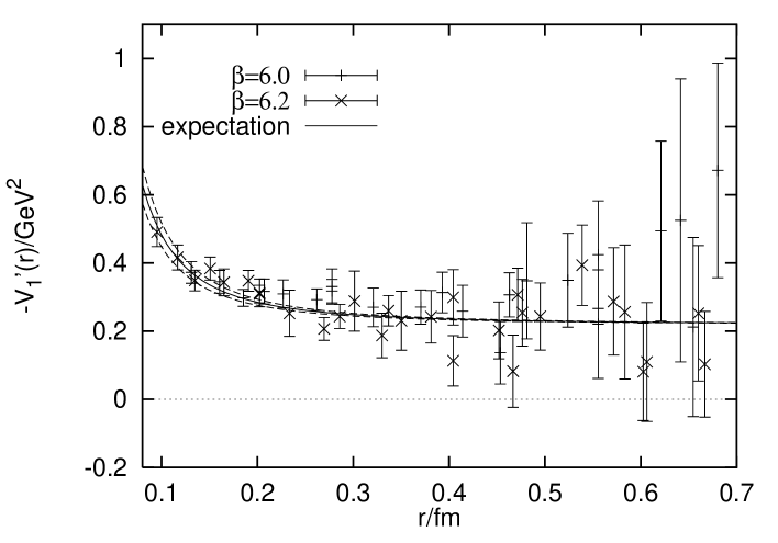
FIG. 10.: The spin-orbit potential $V_{1}^{\prime}$, together with a fit curve of the form $-V_{1}^{\prime}(r)=\kappa+h/r^{2}$. with $h=0.067(9)$.

FIG. 11.: The spin-orbit potential $V_{2,\mbox{cont}}^{\prime}$ in comparison to the continuum expectation from Eq. (134).

FIG. 12.: The spin-spin potential $V_{3,\mbox{cont}}$ in comparison to the continuum expectation from Eq. (135).

FIG. 13.: The spin-spin potential $\tilde{V}_{4}$ for the two $\beta$-values in lattice units.

FIG. 14.: The MD potential $V_{b,\mbox{cont}}$ in comparison to the continuum expectation from Eq. (100).

FIG. 15.: The MD potential $-V_{c,\mbox{cont}}$ in comparison to the continuum expectation from Eq. (100).

FIG. 16.: The MD potential $-V_{d}$ in comparison to the continuum expectation from Eq. (101). The constants $C_{d}$ have been subtracted from the data points.

FIG. 17.: The MD potential $-V_{e}$ in comparison to the continuum expectation from Eq. (101).

FIG. 18.: Comparison of the lattice potential $\tilde{V}_{2}^{\prime}$ at $\beta=6.2$ to tree-level lattice perturbation theory [Eq. (70)] and to the one-loop model of Eq. (149).

FIG. 19.: Same as Fig. 18 for $\tilde{V}_{3}$ [Eqs. (71) and (72)].

FIG. 20.: Same as Fig. 18 for $\tilde{V}_{4}$ [Eq. (73)].

FIG. 21.: Comparison of the lattice potential $-\hat{V}_{c}$ at $\beta=6.2$ to tree-level lattice perturbation theory, Eq. (75).

FIG. 22.: The bottomonium spectrum. The $e=0.32$ results are from the $\beta=6.2$ analysis.

FIG. 23.: The charmonium spectrum. The $e=0.32$ results are from the $\beta=6.2$ analysis.

FIG. 24.: Bottomonium wave functions.