ON THE PATH INTEGRAL LOOP REPRESENTATION OF (2+1) LATTICE NON-ABELIAN GAUGE THEORIES

Abstract

A gauge invariant Hamiltonian representation for SU(2) in terms of a spin network basis is introduced. The vectors of the spin network basis are independent and the electric part of the Hamiltonian is diagonal in this representation. The corresponding path integral for SU(2) lattice gauge theory is expressed as a sum over colored surfaces, i.e. only involving the $j_{p}$ attached to the lattice plaquettes. This surfaces may be interpreted as the world sheets of the spin networks In 2+1 dimensions, this can be accomplished by working in a lattice dual to a tetrahedral lattice constructed on a face centered cubic Bravais lattice. On such a lattice, the integral of gauge variables over boundaries or singular lines – which now always bound three coloured surfaces – only contributes when four singular lines intersect at one vertex and can be explicitly computed producing a 6-j or Racah symbol. We performed a strong coupling expansion for the free energy. The convergence of the series expansions is quite different from the series expansions which were performed in ordinary cubic lattices. In the case of ordinary cubic lattices the strong coupling expansions up to the considered truncation number of plaquettes have the great majority of their coefficients positive, while in our case we have almost equal number of contributions with both signs. Finally, it is discused the connection in the naive coupling limit between this action and that of the B-F topological field theory and also with the pure gravity action.

I Introduction

The loop approach to abelian quantum gauge theories was introduced in the early eighties [1]. Later it was generalized to the non-abelian Yang-Mills gauge theory [2]. This Hamiltonian method allows to formulate gauge theories in terms of their natural physical excitations: the loops. The original aim of this general description of gauge theories was to avoid gauge redundancy working directly in the space of the gauge invariant excitations. However, soon it was realized that the loop formalism goes far beyond of a simple gauge invariant description. The introduction by Ashtekar [3] of a new set of variables that cast general relativity in the same language as gauge theories allowed to apply loop techniques as a natural non-perturbative description of Einstein’s theory. In particular, the loop representation appeared as the most appealing application of the loop techniques to this problem [4].

Recently a Lagrangian approach in terms of loops has been developed for the U(1) model [5], and generalized to include matter fields [6]. The resulting action is proportional to the quadratic area of the loop worldsheet. This allows for Monte Carlo simulations in a more efficient way than by using the gauge potentials as variables. While in the abelian case the usual Hamiltonian in the loop representation can be deduced from the loop action by means of the transfer matrix analisis, the relation between the two approaches is more obscure in the non-abelian case. In fact, the type of surfaces that appear in the Lagrangian loop formulation suggest that the pass to the Hamiltonian can be made simpler if we take a representation different from the loop representation but that shares important features like the use of gauge invariant geometrical objects known as “spin networks”[7]. A spin network basis may be obtained by considering linear combinations of loops. While the loop basis is overcomplete and therefore is constrained by a set of identities known as the Mandelstam identities, the vectors of spin network basis are independent. Furthermore the electric part of the Yang-Mills Hamiltonian is diagonal in spin network space.

A path integral formulation of $SU(2)$ gauge theories in terms of the worldsheets swept out by spin networks has been developed in [8] and [9]. The worldsheets are branched, coloured surfaces, known in the mathematical literature as spines [10]. Such surfaces were introduced in the seventies [11] in the context of strong coupling calculations in Yang-Mills theory. The starting point was a character expantion of the Wilson action. This expantion leads after integration on the link variables to a sum of contributions proportional to the coupling constant raised to a power proportional to the area of closed coloured surfaces. Each coloured surface corresponds to a diagram having a certain number of plaquettes. In the usual hypercubic lattice formulation [11] the higher order terms in the expansion become extremely complicated, discourageing attempts to reformulate gauge theories directly in terms of the coloured surfaces. The main difficulty lies in the computation of certain group theoretic factors for each surface. Nevertheless it is possible to reformulate gauge theories in terms of the surfaces along these lines [8].

In the present paper we show that most of the complications of the group theoretic factors can be avoided by working on a special class of non-cubic lattices, namely the duals to tetrahedral lattices. This leads to an easy calculation of the action of spin network worldsheets, and also simplifies the explicit calculation of strong coupling expansions.

The loop actions of the abelian gauge theories are written in terms of the surfaces swept by the time evolution of the loops. The explicit form of the loop actions for lattice non abelian gauge theories is known to be related with coloured surfaces [8],[9], known as spines in the mathematical lenguage [10]. They are related with the world sheet swept by the evolution in time of the spin networks. However, a complete Lagrangian lattice formulation associated with the spin network representation is not available up to now.

Coloured surfaces were introduced in the seventies [11] to study the strong coupling regime of Yang-Mills gauge theories. The starting point was a character expantion of the Wilson action. This expantion leads after integration on the link variables to a sum of contributions proportional to the coupling constant raised to a power proportional to the area of closed coloured surfaces. Each coloured surface corresponds to a diagram having a certain number of plaquettes. In the usual square lattice formulation [11] the explicit form of the general term of this infinite sum is not known and therefore the action cannot be rewritten in terms of coloured surfaces. The main difficulty relies in the computation of the group theoretic factors of each diagram. In this paper we show that the introduction of a tetrahedral lattice allows to find a very simple expression for these factors and therefore to write the path integral corresponding to the loop representation of the non abelian gauge theories.

In section II we discuss the spin network Hamiltonian approach to Yang-Mills theory. In section III we study the character expansion of the Wilson action and we show why the group factors do not allow to get a closed form for the action in terms of coloured surfaces. In section IV we show that these factors may be simply computed in a tetrahedral lattice where the Wilson action and the Heat Kernel action take a very simple form. In section V we apply this action to perform a strong coupling expantion for the heat kernel version of the theory and we compute the free energy density $f$ and the average plaquette $P$. Finally, in section VI we conclude with some comments on further developments.

II Spin network representation

We consider the pure gauge theory with gauge group $G$ semisimple and compact ($G=U(1)$ or $SU(n)$). We start with the Hilbert space ${\cal H}=\otimes_{\ell}{\cal H}_{\ell}$ where ${\cal H}_{\ell}=L_{2}(G)$ and $\ell$ denote the links of the lattice . On every link $\ell$ we take the “position” basis $|U_{\ell}>$ labelled by the fundamental representation matrices $U_{\ell}\in G$. A basis of ${\cal H}$ is given by the vectors $|U>=\otimes_{\ell}|U_{\ell}>$. Links are oriented and $U_{\bar{\ell}}=U_{\ell}^{-1}$.

A gauge transformation is specified by a group element $V_{s}$ on every lattice site $s$. The state $|U>$ is transformed into $|U^{\prime}>$ where $U^{\prime}_{\ell}=V_{s_{1}}U_{\ell}V_{s_{2}}^{-1}$, $s_{1}$ and $s_{2}$ being the origin and end of $l$. The physical states are those that are invariant under gauge transformations and they define the physical Hilbert space ${\cal H}_{phys}$.

The position and momentum operators $\hat{U}_{\ell}$, $\hat{E}^{a}_{\ell}$ are defined

$$\hat{U}_{\ell}|U>=U_{\ell}|U>$$ (1)

$$e^{i\theta^{a}\hat{E}^{a}_{\ell}}|U>=|U^{\prime}>\,,$$ (2)

where $U^{\prime}_{\ell}=e^{i\theta^{a}T^{a}}U_{\ell}$, $T^{a}$ are generators of the group satisfying

$${\rm Tr}(T^{a}T^{b})=\frac{\delta^{ab}}{2}$$ (3)

$$[T^{a},T^{b}]=ic^{abc}T^{c}.$$ (4)

The reference state $|0>=\int dU|U>$ is gauge invariant and permits to express any state $|\psi>=\psi(\hat{U})|0>$. To work in the physical space ${\cal H}_{phys}$ we have to find a basis $|\psi_{\alpha}>$, that is, a collection of appropiate gauge invariant functions $\psi_{\alpha}(U)$.

One choice is to consider polinomials

$$\prod_{\ell}(U_{\ell})_{a_{1}b_{1}}\cdots(U_{\ell})_{a_{r}b_{r}}(U_{\ell}^{-1})_{c_{1}d_{1}}\cdots(U_{\ell}^{-1})_{c_{s}d_{s}}.$$ (5)

Imposing gauge invariance leads to contraction of indices of incoming and outcoming matrices at every site. The result is the loop representation. That is, states

$$|C_{1},C_{2},\ldots,C_{M}>=W(C_{1})W(C_{2})\cdots W(C_{M})|0>,$$ (6)

where $C_{i}$ are closed loops and

$$W(C)={\rm Tr}\prod_{\ell\in C}U_{\ell}.$$ (7)

These states generate ${\cal H}_{phys}$ but they are not independent. They satisfy the so called Mandelstam constraints which for $SU(2)$ read

$$W(C_{1})W(C_{2})=W(C_{1}C_{2})+W(C_{1}\overline{C}_{2}),$$ (8)

for every two loops $C_{1},C_{2}$ with the same origin.

Instead of (5) we can consider the states given by functions

$$\prod_{\ell}D^{(\mu_{\ell})}_{a_{\ell}b_{\ell}}(U_{\ell})\,,$$ (9)

where $\mu$ runs over the irreducible representations of $G$ and $D^{(\mu)}$ are the matrices of these representations. (Links in the trivial representation are not mentioned explicitly.) Looking to a vertex where enter links in the $\mu_{1},\ldots,\mu_{r}$ representations and leave links in the $\nu_{1},\ldots,\nu_{s}$ representations we have functions

$$D^{(\mu_{1})}_{a_{1}b_{1}}(U_{1})\cdots D^{(\mu_{r})}_{a_{r}b_{r}}(U_{r})D^{(\nu_{1})}_{c_{1}d_{1}}(V_{1})\cdots D^{(\nu_{s})}_{c_{r}d_{r}}(V_{r})\lambda[^{\mu_{1}}_{b_{1}}\cdots^{\mu_{r}}_{b_{r}}|^{\nu_{1}}_{c_{1}}\cdots^{\nu_{s}}_{c_{s}}]\,,$$ (10)

where $\lambda[\cdots]$ are coeficients that ensure gauge invariance. (We sum over repeated latin indices.) If we perform a gauge transformation with element $g$ at the present site we see that $\lambda$ must be an invariant tensor

$$\lambda[^{\mu_{1}}_{a_{1}}\cdots^{\mu_{r}}_{a_{r}}|^{\nu_{1}}_{d_{1}}\cdots^{\nu_{s}}_{d_{s}}]=$$

$$D^{(\mu_{1})}_{a_{1}b_{1}}(g^{-1})\cdots D^{(\mu_{r})}_{a_{r}b_{r}}(g^{-1})D^{(\nu_{1})}_{c_{1}d_{1}}(g)\cdots D^{(\nu_{s})}_{c_{r}d_{r}}(g)\lambda[^{\mu_{1}}_{b_{1}}\cdots^{\mu_{r}}_{b_{r}}|^{\nu_{1}}_{c_{1}}\cdots^{\nu_{s}}_{c_{s}}].$$ (11)

The $\lambda$ tensors can be computed from the Clebsh-Gordan coeficients for the group. The condition for $\lambda$ being non zero is that the decompositions of the product of the representations entering and the product of the representations leaving have common terms. We note also that the maximum number of links associated to a given site is small and varies with the dimension of the space so the order of these tensors are bounded. The representation defined by these states is called spin network representation. The states are represented graphically as oriented paths with branching points where every single line is labelled by a representation of the group

FIG. 1.:

Supose now that the group is abelian ($G=U(1)$). Then the irreducible representations are one-dimensional and have the form $D^{(n)}(U)=U^{n}$ for $n\in{\bf Z}$. So the (9) states coincide with the polinomial states (5) and the loop representation and the spin network representation are the same.

For non abelian $G$ the two representations are different. It is clear that a site can not have only one link entering or only one link leaving. The simplest case is one link entering and another link leaving. Both must be in the same representation and the invariant tensor is

$$\lambda[^{\mu}_{a}|^{\mu}_{d}]=\delta_{ad}.$$ (12)

The efect of this tensor is to multiply the matrices that enter and leave so single lines in the spin network are labeled by a single representation. The case of two links entering a site is forbiden in general but in the case of $SU(2)$ there are invariant tensors like $\epsilon_{ab}$ (antisymmetric and $\epsilon_{12}=1$). The efect of these tensors is to reverse one of the lines converging on the site. This is due to the fact that for $SU(2)$ every representation is equivalent to its conjugate.

When three lines meet in a site the condition for the existence of non zero invariant tensors is that the product of the entering representations contains the trivial representation. In that case the invariant tensor is given by the CG coeficients

$$D^{(\mu)}_{ab}(g)D^{(\nu)}_{cd}(g)=\sum_{\rho}C(\mu a,\nu c|\rho d)D^{(\rho)}_{de}(g)C(\rho e|\mu b,\nu d)\,,$$ (13)

which are taken real

$$C(\mu a,\nu b|\rho c)=C(\rho c|\mu a,\nu b).$$ (14)

As we consider only simply reducible groups no other independent invariant tensor exists. Then the state corresponding to a trivalent vertex is well encoded in the drawing of the spin network. This is not in general the case for sites where meet four or more lines. The dimension of the space of invariant tensors is the number of times that the product of the entering representations contains the trivial representation. Besides the spin network it must be provided information about which tensors we select on the vertices. This degeneration is not fundamental since these vertices can be thought as the limiting case when the line connecting two trivalent vertices gets zero lenght.

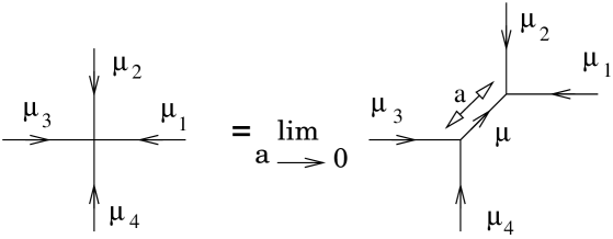
FIG. 2.:

The Hamiltonian operator is

$$H=\frac{g^{2}}{2}\sum_{\ell}\hat{E}_{\ell}^{2}-\frac{1}{2g^{2}}\sum_{p}(W(p)+W(\bar{p}))\,,$$ (15)

where $g$ is the coupling constant, $\ell$ and $p$ are the links and plaquettes of the lattice respectively, $\hat{E}_{\ell}^{2}=\hat{E}_{\ell}^{a}\hat{E}_{\ell}^{a}$ and $W(p)$ is given by (7). The fundamental commutation relations are ($T^{(\mu)}_{a}$ are the generators of the $\mu$ irred. rep.):

$$[\hat{E}_{\ell}^{a},D^{(\mu)}(\hat{U}_{\ell}^{\prime})]=-T^{(\mu)}_{a}D^{(\mu)}(\hat{U}_{\ell})\delta_{ll^{\prime}}+D^{(\mu)}(\hat{U}_{\ell}^{\prime})T^{(\mu)}_{a}\delta_{\bar{l}l^{\prime}}$$ (16)

$$[\hat{E}_{\ell}^{a},\hat{E}_{\ell}^{b}]=ic^{abc}\hat{E}_{\ell}^{c}.$$ (17)

A spin network state is denoted ${\cal N}=P_{1}P_{2}\cdots P_{M}$ where $P_{i}$ are the single lines. $\mu_{i}$ is the representation carried by line $P_{i}$. We get for the action of the electric part of the Hamiltonian:

$$\sum_{\ell}\hat{E}_{\ell}^{2}|{\cal N}>=L({\cal N})|{\cal N}>\,,$$ (18)

$$L({\cal N})=\sum_{i}c^{(\mu_{i})}L(P_{i})\,,$$ (19)

where $L(P_{i})$ is the number of links in the line $P_{i}$ and $c^{(\mu)}$ is the quadratic Casimir number of the representation given by $T^{(\mu)}_{a}T^{(\mu)}_{a}=c^{(\mu)}Id$. For example, for $SU(2)$, $c^{(j)}=j(j+1)$ .

Then the spin network states, in contrast to the loop states, are always eigenstates of the electric term.

The magnetic part produces deformations of the spin networks both in the geometrical shape and the representations of the lines. This is represented graphically:

FIG. 3.:

The spin network states $|\cal{N}>$ are independent and orthonormal. A proof using an inner product structure on the state space is given in [7]. Loop states can be expanded in spin network terms in a unique way so the Mandelstam constrains disappear when we pass to the spin network representation.

To further clarify the relation between loop and spin network states we recall the action of the electric part of the Hamiltonian over a loop state (6)

$$\sum_{\ell}\hat{E}_{\ell}^{2}|C_{1},C_{2},\ldots,C_{M}>=$$

$$(nL(C_{1},C_{2},\ldots,C_{M})-\frac{1}{n}\Lambda(C_{1},C_{2},\ldots,C_{M}))|C_{1},C_{2},\ldots,C_{M}>$$

$$+\sum_{i}\sum_{l,l^{\prime}}\bar{\delta_{l,l^{\prime}}}|C_{1},\ldots,C_{ixy},C_{iyx},\ldots,C_{M}>$$

$$+2\sum_{i<j}\sum_{l\in C_{i}}\sum_{l^{\prime}\in C_{j}}\bar{\delta_{l,l^{\prime}}}|C_{1},\ldots,(C_{ixx}C_{jyy}),\ldots,C_{M}>\,,$$ (20)

where $L(C_{1},C_{2},\ldots,C_{M})$ is the number of links in the set of loops taking acount of the multiplicity (single lenght), and $\Lambda(C_{1},C_{2},\ldots,C_{M})$ is the sum of the squares of these multiplicities (quadratic lenght). $\bar{\delta}_{l,l^{\prime}}$ is 1 if $l=l^{\prime}$ and $-1$ if $\bar{l}=l^{\prime}$ and $x,y$ are the edges of $l$.

In equation (20) we see that in general the loop states are not eigenstates of the electric operator. The last two sums are geometric interaction terms: fusions where a loop splits into two components and fisions where two loops join in a common link.

III The Wilson action in a cubic lattice

The path integral for the Wilson action for a general non-Abelian compact gauge group G is given by

$$Z_{W}=\int[dU_{\ell}]\exp[{\beta\sum_{p}\mbox{Re}({\rm Tr}U_{p})\,]},$$ (21)

where the $U_{\ell}\in G$ and $U_{p}=\prod_{\ell\in p}U_{\ell}$.

The analogous of the Fourier expansion for the non-Abelian case is the character expansion. The characters $\chi_{r}(U)$ of the irreducible (unitary) representation $r$ of dimension $d_{r}$, defined as the traces of these representations, are an orthonormal basis for the class functions of the group i.e. [11]

$$\int dU\chi_{r}(U)\chi_{s}^{*}(U)=\delta_{rs}$$ (22)

$$\sum_{r}d_{r}\chi_{r}(U{V^{-1}})=\delta(U,V).$$ (23)

In particular, as a useful consequence we have

$$d_{r}\int dU\chi_{s}(U)\chi_{r}(U{V^{-1}})=\delta_{rs}\chi_{r}(V).$$ (24)

By means of the character expansion we can express

$$\exp\{\beta\sum_{p}\mbox{Re}[{\rm Tr}U_{p}\,]\}=\prod_{p}\sum_{r}c_{r}\chi_{r}(U_{p}),$$ (25)

with

$$c_{r}=\int dU\chi_{r}^{*}(U)\exp{(\beta{\rm Tr}U\,)}.$$ (26)

In the case of $G=SU(2)$ a direct application of (26) yields the $c_{j}$ in terms of modified Bessel functions, and therefore we can express (21) as

$$Z_{W}=\int[dU_{\ell}]\prod_{p}[\sum_{j_{p}}2(2j_{p}+1)\frac{I_{2j_{p}+1}(\beta)}{\beta}\chi_{j_{p}}(U_{p})]$$ (27)

$$=\sum_{\{j_{p}\}}\prod_{p}[2(2j_{p}+1)\frac{I_{2j_{p}+1}(\beta)}{\beta}]\int[dU_{\ell}]\prod_{p}\chi_{j_{p}}(U_{p}).$$ (28)

It will be convenient to introduce the following quantities in order to rewrite the path integral $Z_{W}$

$$c_{0}=\frac{2I_{1}(\beta)}{\beta},$$ (29)

$$c_{0}\beta_{j}=\frac{2I_{2j+1}(\beta)}{\beta}.$$ (30)

The path integral takes the form,

$$Z_{W}={c_{0}}^{N}\int{\prod_{p}[1+\sum_{j_{p}\neq 0}(2j_{p}+1)\beta_{j_{p}}\chi_{j_{p}}(U_{p})]}\prod_{\ell}dU_{\ell}$$ (31)

where $N$ is the number of plaquettes.

Let us now show how the sum over coloured surfaces arise in $Z_{W}$. A given subset of plaquettes carring $j_{p}\neq 0$ is homeomorphic to a simple surface if any link bounds at most two plaquettes of this subset. The links bounding exactly one plaquette make up the free boundary of this surface. Any configuration can be decomposed as a set of maximal simple surfaces by cutting it along the links bounding more than two plaquettes. In principle, there are two possibilities for the boundary curves: either a free boundary, bounding only one simple surface or a singular branch line along which more than two simple surfaces meet. In fact, relation (22) forbids the existence of free boundaries for non trivial configurations contributing to the path integral.

The integration over the internal links of the simple surfaces is performed using (24). Note that the plaquettes of a simple surface component should carry the same group representation. After integrating over all the inner links of the simple components one gets [12] an expression involving only the links of the boundaries,

$$Z_{W}=c_{0}^{N}\sum_{\mbox{{spines}}}{\int{(\prod_{l\in\partial A}dU_{\ell}}})\prod_{i}{\beta_{j_{i}}}^{A_{i}}(2j_{i}+1)^{\epsilon_{i}}\prod_{\mbox{{boundaries}}}{\chi_{j_{i}}[\partial A_{i}]}\,,$$ (32)

where $\epsilon_{i}$ is the Euler’s topological invariant of the surface $i$ with area $A_{i}$. Euler’s characteristic is explicitly given by:

$$\epsilon=n_{2}-n_{1}+n_{0}=2-2g-b$$ (33)

where $n_{2}$ is the number of plaquettes, $n_{1}$ the number of distict links bordering these plaquettes and $n_{0}$ the number of end points of these links, $g$ is the genus of the surface and $b$ the number of boundaries.

An important property of the character expansion (28), relevant for strong coupling expansions is that only a finite number of terms in 25 contribute to a given order in $\beta$. In fact,

$$c_{r}=O[\beta^{\nu}_{r}]$$ (34)

where $\nu_{r}$ is the smallest integer such that $\chi^{\nu}(U)$has a non vanishing component along $\chi_{r}(U)$.In the SU(2) case $\nu_{j}=2j$.

In [8] and [9] a path integral over coloured surfaces is obtained along the lines described here. However, on a cubic lattice the group factors of the surfaces are difficult to compute because with up to four surfaces meeting at singular lines, and up to six singular lines meeting at points, the integral in (27) can be very complicated, involving recoupling coefficients of up to 12 $j$s. That is way these group factors has been only perturbatively computed for the diagrams that appear in the strong coupling expantion.

Working with a cubic lattice is equivalent to work with spin networks involving four valent vertices in the Hamiltonian approach discussed in section II. In this case, it is well known that only three valent vertices have an unambigous correspondence with the information encoded in the drawing of the spin network. Higher order vertices require additional information about the invariant tensor used to couple the irreducible representations. At the action level this means that additional group factors associated with different ways of coupling the coloured surfaces at singular lines appear. In [8] this problem is dealt with by assigning colours to the singular lines which are summed over in the path integral. However, this complication may be avoided by using a special class of lattices. In the dual to a tetrahedral lattice only three plaquettes meet at each link, so singular lines involve at most three coloured surfaces.

IV Loop actions in tetrahedral lattices

In order to introduce the tetrahedral lattice above mentioned, some concepts of solid state physics are very useful [13]. The Bravais lattice is one of such concepts; it specifies the periodic array in which the repeated units of a crystal are arranged. That is, the Bravais lattice summarizes the geommetry of the underlying periodic structure, regardeless of what the actual units be (single atoms, molecules, groups of atoms, etc.). A (three-dimensional) Bravais lattice is specifyed by three vectors a₁, a₂ and a₃ called primitive vectors. The primitive vectors generate all the traslations such that the lattice appears exactly the same. The primitive unit cell generated by the primitive vectors often does not have the full symmetry of the Bravais lattice. However, one can always consider a nonprimitive unit cell, known as conventional unit cell, which is generally chosen to be bigger than the primitive cell and such that to have the full symmetry of their Bravais lattice.

Le us consider a face centered cubic Bravais lattice – i.e. the lattice obtained when one adds to the simple cubic lattice an aditional point in the center of each square face – with primitive vectors ${\bf a_{1}}=a({\bf i+j}),{\bf a_{2}}=a({\bf j+k}),{\bf a_{3}}=a({\bf k+i})$ The conventional unit cell of this lattice is a cube of side $2a$ with a four point basis located at $(0,0,0),(a,0,0),(0,a,0)(0,0,a)$ Translations along the primitive vectors generate 27 points associated with 8 cubes of side $a$ in the conventional cell.The Bravais conventional unit cell with the four basis points and the eight cubes is depicted in FIG. 4.

FIG. 4.:

Each cube of side $a$ may be decomposed in the five tetrahedra $ABDE,\;CBDG,\;EBGE,\;HDGE,$ and $EBGD$ as shown in FIG. 5. The links of the lattice are the edges of these tetrahedra. The first four tetrahedra has volume $a^{3}/6$ while the last one has volume $2a^{3}/6$. If the vertex $A$ of the cube depicted in FIG. 5 has coordinates(0,-a,0) the other cubes are obtained by symmetizing with respect to the planes $Exy,\;Eyz,\;Ezx$ and traslating along the primitive vectors. Coloured surfaces will be associated to the plaquettes of the dual lattice.The vertices of this lattice are the centers of the tetrahedra:

$$X_{A}({\bf\epsilon})=\frac{a}{4}(\epsilon_{1},3\epsilon_{2},\epsilon_{3})$$ (35)

$$X_{C}({\bf\epsilon})=\frac{a}{4}(3\epsilon_{1},3\epsilon_{2},3\epsilon_{3})$$ (36)

$$X_{F}({\bf\epsilon})=\frac{a}{4}(3\epsilon_{1},\epsilon_{2},\epsilon_{3})$$ (37)

$$X_{H}({\bf\epsilon})=\frac{a}{4}(\epsilon_{1},\epsilon_{2},3\epsilon_{3})$$ (38)

$$X_{O}({\bf\epsilon})=\frac{a}{2}(\epsilon_{1},\epsilon_{2},\epsilon_{3})$$ (39)

where $\epsilon=\pm 1$

FIG. 5.:

Each cell contains one polyhedron with 12 hexagonal faces and six squared faces. In FIG. 6 we show the points and links of one polyhedron and one cube. Translations along the primitive vectors fill all the lattice. Each of the squares is a face of one cube of side $a/2$. We shall attach a $SU(2)$ group element $U_{\ell}$ in the fundamental representation to each link of this lattice.

FIG. 6.:

Now let us consider the Wilson action defined in terms of the plaquettes of this lattice.

$$S=\beta[\sum_{p_{s}}{\rm Re}({\rm Tr}U_{p_{s}})+\sum_{p_{h}}{\rm Re}({\rm Tr}U_{p_{h}})]$$ (41)

where $U_{p_{s}}$ and $U_{p_{h}}$ respectively are the holonomies for the squared and hexagonal plaquettes.

One can show that this action has the correct continum limit for $a$ going to zero, leading to the classical Yang-Mills action.

One can repeat the same steps leading two (32), but now the singular lines always bound three coloured surfaces. In this case the integral along the boundaries in (32) only contributes when four singular lines intersect at one point and may be explicitly computed. Let us call $S_{k}$ the intersecting point and $\gamma_{1},...\gamma_{4}$ the singular lines intersecting at $S_{k}$. Then we have six coloured surfaces with colours $j_{12},j_{13},j_{14},j_{23},j_{24}$ and $j_{34}$ bounded by these lines. That means that in the original tetrahedral lattice we shall have a tetrahedrom with one of the values of $j$ on each edge. The exact path integral may now be written in terms of a sum over coloured surfaces.

$$Z_{W}=c_{0}^{N}\sum_{spines}\prod_{i}{\beta_{j_{i}}}^{A_{i}}(2j_{i}+1)^{\epsilon_{i}}\prod_{S_{k}}{(-1)^{\sum_{i}j_{ii+1}^{k}}}\left\{\begin{array}[]{lll}j_{12}^{k},&j_{13}^{k},&j_{14}^{k}\\ j_{34}^{k},&j_{24}^{k},&j_{23}^{k}\end{array}\right\}$$ (42)

where the six $j$ symbols are the Racah coefficients and the exponent of $-1$ denotes the cyclic sum $j_{12}+j_{23}+j_{34}+j_{41}$.

A simpler but equivalent action may be obtained starting from the Heat Kernel path integral

$$Z_{HK}=\int[dU_{\ell}]\prod_{p}[\sum_{j_{p}}(2j_{p}+1)\exp\left\{-\frac{j_{p}(j_{p}+1)}{2\beta}\right\}\chi_{j_{p}}(U_{p})]\,.$$ (43)

By following the same steps one gets the same expression for the path integral in terms of coloured surfaces (42) with $c_{0}=1$ and $\beta_{j}=\exp\{-[j(j+1)/2\beta]A_{j}\}$.

V Strong coupling expansions

Our aim in this section is to show that the introduction of the previous Bravais lattice not only allows to perform calculations but also simplify them. Therefore, we will show here how to perform a strong coupling expansion. In order to do so we will use, just for simplicity, the expression for the path integral in terms of coloured surfaces which corresponds to the Heat Kernel action:

$$Z=\sum_{spines}\prod_{i}\exp\left\{-\frac{j_{i}(j_{i}+1)}{2\beta}A_{i}\right\}(2j_{i}+1)^{\epsilon_{i}}\prod_{S_{k}}{(-1)^{\sum_{i}j_{ii+1}^{k}}}\left\{\begin{array}[]{lll}j_{12}^{k},&j_{13}^{k},&j_{14}^{k}\\ j_{34}^{k},&j_{24}^{k},&j_{23}^{k}\end{array}\right\}.$$ (44)

We will follow an analogous treatment to that of Drouffe and Zuber [12]. We will expand in powers of the $t$ parameter given by $t\equiv e^{-\frac{1}{4\beta}}$.

Free energy density f

The free energy density $f=F/N$, where $F$ is the free energy and $N$ the number of plaquettes, is obtained by summing the terms linear in N in the expansion of the path integral (44) in powers of $t$. The power of $t$ of each diagram (volumes in three space-time dimensions) is equal to

$$\sum_{r}2j_{r}(j_{r}+1)\times n_{r}$$

where $j_{r}$ denotes the representations of the group SU(2) or “colours” and $n_{r}$ denotes the number of plaquettes (square plaquettes + hexagonal plaquettes) of the the diagram. For instance, the first power of the expansion corresponds to the smallest volume, i.e. the cube, with all their plaquettes with $j=\frac{1}{2}$ and it gives a power of 2$\times\frac{3}{4}\times 6=9$; the next power is produced by two disconnected cubes (recall that in our lattice cubes make contact only with polyedra) with $j=\frac{1}{2}$ which gives a power of 18 and so forth. The contribution of each diagram to $f$ can be written as the product of two numbers: the reduced configuration number (r.c.n.) times a group theoretical factor [12]. To compute the r.c.n. one has to count the number of inequivalent positions of a given diagram on the lattice – its configuration number – and then to extract the term linear in $N$ which is the r.c.n. The group theoretical factors stem from the integrations over the link variables $U_{\ell}$ and their general form is

$$\sum_{r\neq 0}d_{r}^{n_{2}-n_{1}+n_{0}}\prod_{\mbox{{boundaries}}}\chi_{r}(U_{\mbox{{boundary}}}),$$

where $d_{r}$ is the dimension of the representation $r$, $n_{2}$ is the number of plaquettes with $j=j_{r}$, $n_{1}$ the number of distinct links bordering these plaquettes and $n_{0}$ the number of endpoints of these links. For example, diagrams with the topology of a sphere give contributions $\sum_{r\neq 0}d_{r}^{2}$. The main advantage of the introduced lattice is that the group theoretical factors for more complicated diagrams can always be explicitely expressed in terms of the $d_{r}$ and 6-$j$ Racah symbols. The Racah symbols arise each time four singular lines meet at one vertex and they appear in the diagrams by pairs. The first of this pairs come out in the diagram of two polyhedron sharing an hexagonal face and a cube sharing two of its contiguous faces, one with each polyhedron (FIG. 7).

FIG. 7.:

All the external 36 plaquettes of this diagram are labeled with $j=\frac{1}{2}$ while the 3 internal (shared) plaquettes are labeled with $j=1$; then it gives a power of $t^{\frac{3}{2}\times 36+4\times 3}=t^{66}$. We have computed the strong coupling expansion of $f$ up to power 53 in $t$ which involves 34 diagrams grouped in 18 different powers of $t$:

$$f=4t^{9}-8t^{18}+9t^{24}+76/3t^{27}-12t^{33}-160t^{36}+72t^{37}+60t^{39}$$ (45)

$$-432t^{42}+360t^{43}+8224/5t^{45}+612t^{46}-1728t^{47}-2961/2t^{48}$$ (46)

$$+720t^{49}+5052t^{51}-8640t^{52}+2664t^{53}$$ (47)

We plot in FIG. 8 the $f$ vs. $\beta$ for different powers of truncation of the expansion.

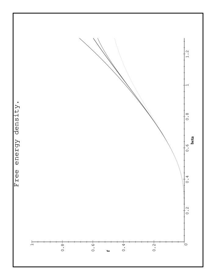
FIG. 8.: Free energy $f$ vs. $\beta$ for several truncation orders. From above: $t^{27}$, $t^{39}$, $t^{46}$, $t^{53}$ and $t^{18}$.

As long as we enter in the weak coupling regime ($\beta>1$), one can appreciate a clear difference with the series expansions of ref. [12] which were performed in an ordinary cubic lattice and with a different truncation criteria (they consider diagrams up to 16 plaquettes which corresponds to $t^{24}$). The explanation of this difference relies on the fact that in the strong coupling expansion in a cubic lattice up to 16 plaquettes all the terms except two are positive while in our case we have almost equal number of contributions with both signs.

Thus, one can observe that the introduction of the dual of the tethraedral lattice, besides simplifiying the strong coupling computations provides a straightforward procedure to obtain the desired terms of the series expansion. This turns to be an advantage in order to reach the weak coupling regime.

VI CONCLUSIONS

We have introduced a Hamiltonian spin network representation for a SU(2) lattice gauge theory. This gauge invariant representation is given in terms of an independent basis that diagonalize the electric part of the Hamiltonian. The corresponding Lagrangian formulation is also developed. This formulation takes a purely geometrical form in terms of sums over coloured surfaces and allow to combine the powerfull Lagrangian techniques with the redundancy free description typical of the loop representation. This action may be written on a thetrahedral lattice explicitly in terms of the Racah coefficients. The computation of group theoretical factors of diagrams of the strong coupling expansion of high orders of $t$ becomes straigtforward, only involving these Racah coefficients. Also, we have a compact expression for the coloured surfaces action which allows to perform numerical computations.

In the naive weak coupling limit, the area dependent factors become equal to 1 and the action is purely topological. One can immediately check that this limit correspond to the Ouguri [14] form of the B-F topological field theory, which in three dimensions is known [15] to coincide with the pure gravity action. In this case the use of the Biedenharn and Elliot identity [16] allows to show that the action is invariant under the renormalization group. Thus, in the different context of QCD, this suggests that the Yang Mills action in terms of coloured surfaces may be particularly well suited for the study of the effective theories.

Even though the method developed here was for SU(2) in 2+1 dimensions, the extension to other groups, in particular to SU(3), is straightforward. The corresponding spin networks would simply carry the quantum numbers required to charactherize the irreducible representations of the Lie group under study. It is also possible to extend this formulation to the four dimensional case, by making use of the higher order Racah-Wigner $j$-coefficients. An important simplification of the path integral (44) with the same weak coupling regime could be obtained by making use of the Ponzano and Regge asymptotic form of the Racah-Wigner $j$-symbols. We hope to present elsewhere a more detailed analysis of these developments.

REFERENCES

- [1] R. Gambini and A. Trias Phys. Rev. D22 (1980) 1380.
- [2] R. Gambini and A. Trias Nucl. Phys. B278 (1986)436.
- [3] A. Ashtekar Phys. Rev. Lett. 57 (1986) 2244; Phys. Rev. D36, (1987) 1587.
- [4] C. Rovelli and L. Smolin, Phys. Rev. Lett. 61 (1988) 1155; Nuc. Phys. B331 (1990) 80.
- [5] J.M. Aroca, M. Baig and H. Fort, Phys. Lett. B336 (1994) 54.
- [6] J.M. Aroca, M. Baig, H. Fort and R. Siri, Phys. Lett. B366 (1995) 416.
- [7] C. Rovelli and L. Smolin, Phys. Rev. D53,5743 (1995)
- [8] M. Reisenberger, gr-qc 9412035 (1994).
- [9] J.M. Aroca, H. Fort and R. Gambini , Phys. Rev. D54 (1996) 7751.
- [10] L.Kauffman and S.Lins, Temperley-Lieb Recoupling Theory and Invariants of 3-Manifolds. Princeton Univ. Press (1994)
- [11] C. Itzykson, J.M. Drouffe in STATISTICAL FIELD THEORY. VOL. 1 Cambridge Univ. Press. (1989).
- [12] J. M. Drouffe and J. B. Zuber, Phys. Rep. 102 (1983) 1, and references therein.
- [13] N.W. Ashcroft and N.D. Mermin, Solid State Physics , Saunders Collage Publishing 1976.
- [14] H. Ouguri, Nucl. Phys. B382 (1992) 276.
- [15] E. Witten, Commun. Math. Phys. 181(1989) 351.
- [16] L.C. Biedenharn, J. Math Phys 31 (1953) 287.