ITFA-97-02
February 1997

Numerical study of plasmon properties in the SU(2)-Higgs model

Abstract

Using the (effective) classical approximation, we compute numerically time-dependent correlation functions in the SU(2)-Higgs model around the electroweak phase transition, for $m_{H}\approx m_{W}$. The parameters of the classical model have been determined previously by the dimensional reduction relations for time-independent correlators. The $H$ and $W$ correlation functions correspond to gauge invariant fields. They show damped oscillatory behavior from which we extract frequencies $\omega$ and damping rates $\gamma$. In the Higgs phase the damping rates have roughly the values obtained in analytic calculations in the quantum theory. In the plasma phase (where analytic estimates for gauge invariant fields are not available), the damping rate associated with $H$ is an order of magnitude larger than in the Higgs phase, while the $W$ correlator appears to be overdamped, with a small rate. The frequency $\omega_{H}$ shows a clear dip at the transition. The results are approximately independent of the lattice spacing, but this appears to be compatible with the lattice spacing dependence expected from perturbation theory.

1 Introduction

The classical approximation has been introduced some time ago in quantum field theory to avoid the difficulties of numerical simulations of time dependent phenomena at high temperature [1]. It is potentially a very powerful method for nonequilibrium phenomena as well. It has been used for the numerical study of the Chern-Simons diffusion rate in the (1+1)D abelian Higgs model [2–7], the (3+1)D SU(2)-Higgs model [8, 9, 10] and pure SU(2) gauge theory [11], as well as in a study of real time properties of the electroweak phase transition [12]. The results have been encouraging. For example, the sphaleron rate in the classical abelian Higgs model obtained by numerical simulations agrees with the analytic expression of quantum field theory [4–7]. In the corresponding pure SU(2) and SU(2)-Higgs cases the rate appeared to be lattice spacing independent in refs. [11, 10], but these results are now considered to be misleading, because of bad ultraviolet properties of the observable used for estimating the Chern-Simons diffusion. Recent simulations with improved observables have led to much better results in the Higgs phase and somewhat different values for the rate in the plasma phase [13, 14]. The case of SU(3) gauge theory has also been studied [15]. However, these new results for the rate show lattice spacing dependence.

A recent analysis of the dynamics of hot quantum gauge fields led to the conclusion that the classical rate should depend on the lattice spacing [16]. Other lattice artefacts such as anisotropies have been anticipated earlier [17]. These have been studied in detail in [18], where a useful fudge factor was derived for converting the rate in the classical theory to an estimate for the rate in the quantum theory. These studies were analytic, based on a separation of scales $gT$, $g^{2}T$, in resummed perturbation theory. This may be questionable when the gauge coupling $g$ is not very small.

In any case, the very validity of the effectively classical approximation for real time processes needs further clarification. For this reason we undertook the present study of correlation functions in the classical SU(2)-Higgs theory. The emphasis here is on time dependent correlation functions. The static correlation functions, which describe the initial conditions of the time dependent ones, have been well studied since they correspond to a dimensional reduction approximation of the quantum theory at high temperature. The static theory can be renormalized, with finite renormalizations determined by matching the classical to the quantum theory [19]. An important question is if the time dependent theory is also renormalizable.

Recently [20], time dependent correlation functions have been studied in hot classical $\phi^{4}$ theory using perturbation theory and it was shown that the ultraviolet divergencies can be absorbed in counterterms, the same mass counterterms as needed in the static theory. This led in particular to a finite classical plasmon damping rate. Matching the parameters of the classical static theory with those in the quantum theory, this classical damping rate was found to agree with the hard thermal loop expression of the quantum theory. Such matching was applied previously to the SU(2)-Higgs model for the computation of the Chern-Simons diffusion rate [10]. The analysis is to be completed by a more detailed comparison between the fully time dependent classical and quantum theories [21].

Our approach is different from propositions based on an effective theory of hard thermal loops [17, 22], in which the cutoff of the classical theory should not be removed. We are instead aiming at the construction of a classical SU(2)-Higgs theory that is renormalizable (as in the scalar case [20]), such that physical results are free of regularization artefacts, for sufficiently large cutoff or small lattice spacing. We do not know yet if such a construction exists. It may involve nonlocal counterterms or other degrees of freedom, e.g. as in [23]. The reason is that in gauge theories the divergences in the classical theory are non local, of a form that is analogous to the hard thermal loops in the quantum theory. Furthermore, the form of the usual classical hamiltonian does not allow for a counterterm to compensate for the divergence in the Debije mass [10]. Also the plasmon frequency is divergent [18]. On the other hand, in the static case, the large Debije mass is the rationale for integrating out the corresponding modes to get a simpler form of the dimensional reduction approximation. Similarly, in the time dependent case, without additional nonlocal counterterms, any modes with divergent frequencies or damping rates may simply decouple from coarse grained large time behavior. The question is, if what is left over can be interpreted as a (nonperturbatively) renormalizable theory.

In this paper we deal with the usual classical model and concentrate on relatively simple time dependent correlation functions. First of all, we want to see if it is feasible to compute such autocorrelation functions numerically with reasonable accuracy, find out how the results depend on the lattice spacing, using the counterterms known from the static theory, and compare with hard thermal loop results of the quantum theory.

Such a comparison is not straightforward in the high temperature phase. In the analytic calculations the correlation functions are constructed from the elementary field variables using gauge fixing, while nonperturbatively one tends to use gauge invariant composite local fields. Even if the final results obtained analytically are gauge invariant, it is not clear that these refer to the same quantities as those obtained with the gauge invariant fields. For example, in the plasma phase there is a large discrepancy between the two cases in the screening masses with $W$ quantum numbers [24-29] (see also the reviews [30, 31] and the interpretation given in ref. [32]). In the Higgs phase the results agree, as can be understood from the usual argument which we now review.

The simplest gauge invariant composite fields (which we also use) read in the continuum

$$H = \varphi^{\dagger}\varphi,\;\;\;\varphi=\left(\begin{array}[]{c}\varphi_{u}\\ \varphi_{d}\end{array}\right),$$ (3)

$$W_{\mu}^{\alpha} = i\mbox{Tr}\,\phi^{\dagger}(\partial_{\mu}-iA_{\mu}^{\beta}\,t_{\beta})\phi\,t_{\alpha},\;\;\;\phi=\left(\begin{array}[]{cc}\varphi_{d}^{*}&\varphi_{u}\\ -\varphi_{u}^{*}&\varphi_{d}\end{array}\right),$$ (6)

with $\varphi$ the Higgs doublet, $A_{\mu}^{\alpha}$ the gauge fields and $t_{\alpha}=\tau_{\alpha}/2$ the SU(2) generators. In the Higgs phase these fields correspond to the usual Higgs and gauge fields. Since $\phi=\sqrt{H}\,V$ with $V\in SU(2)$, $W_{\mu}^{\alpha}$ is essentially the gauge field in the unitary gauge $V=1$, as can be seen in perturbation theory by replacing $\varphi$ by its vacuum expectation value, neglecting fluctuations. This is not useful in the plasma phase where the theory behaves like QCD and perturbation theory runs into infrared problems. Nonperturbatively $H$ and $W_{m}^{\alpha}$ ($m=1,2,3$) are primarily characterized by their behavior under spatial rotations and weak isospin: (scalar,scalar) and (vector,vector), respectively. We have not studied the time component $W^{\alpha}_{0}$, which transforms as (scalar,vector).

To get an idea of the properties of the system being simulated we also computed static correlators of $H$ and $W$ and estimated their screening masses. The temperatures varied around the electroweak transition and parameters were furthermore chosen such that for the zero temperature masses $m_{H}\approx m_{W}$. From the time dependent correlation functions we then attempted to extract plasmon frequencies and damping rates of $H$ and $W$.

We should warn the reader about our terminology. For convenience we often call in this paper the frequencies and attenuation rates associated with the composite $W$ and $H$ fields at zero momentum: ‘plasmon’ frequencies and damping rates. This is controversial, since the terminology ‘plasmon’ is normally associated with the collective modes of the gauge field $A_{\mu}$.

2 Classical SU(2)-Higgs model at finite temperature

We use the same notation as in [10]. The classical SU(2)-Higgs model is defined on a spatial lattice with lattice distance $a$. The parallel transporters (lattice gauge field) are denoted by $U_{m{\bf x}}$, $D_{m}\bar{\varphi}_{{\bf x}}=U_{m{\bf x}}\bar{\varphi}_{{\bf x}+\hat{m}}-\bar{\varphi}_{{\bf x}}$ is the covariant lattice derivative acting on the lattice Higgs doublet $\bar{\varphi}_{{\bf x}}$, $U_{mn{\bf x}}$ is the product of parallel transporters around the plaquette $({\bf x}mn)$. The canonical momenta in the temporal gauge are denoted by $\bar{\pi}$, $\bar{\pi}^{\dagger}$ and $\bar{E}^{\alpha}_{m}$, with nontrivial Poisson brackets

$$\{U_{m{\bf x}},\bar{E}^{\alpha}_{m{\bf x}}\}=iU_{m{\bf x}}\tau_{\alpha},\;\;\;\{\bar{\varphi}_{{\bf x}},\bar{\pi}^{\dagger}_{{\bf x}}\}=1.$$ (7)

The effective classical hamiltonian is given by

$$\frac{H_{\rm eff}}{T} = \bar{\beta}\bar{H},$$ (8)

$$\bar{H} = \sum_{{\bf x}}[\frac{1}{2}\,z_{E}\bar{E}^{\alpha}_{m{\bf x}}\bar{E}^{\alpha}_{m{\bf x}}+z_{\pi}\bar{\pi}^{\dagger}_{{\bf x}}\bar{\pi}_{{\bf x}}+\sum_{m<n}(1-\frac{1}{2}\,\mbox{Tr}\,U_{mn{\bf x}})$$ (9)

$$\mbox{}+(D_{m}\bar{\varphi}_{{\bf x}})^{\dagger}D_{m}\bar{\varphi}_{{\bf x}}+\bar{\lambda}(\bar{\varphi}^{\dagger}_{{\bf x}}\bar{\varphi}_{{\bf x}}-\bar{v}^{2})^{2}],$$

where $T$ is the temperature and $\bar{\beta}$, $\bar{\lambda}$ and $\bar{v}^{2}$ are effective couplings which depend on $a$, $T$ and the couplings in the 4D quantum theory,

$$\bar{\beta} \approx \frac{4}{g^{2}aT},\;\;\;\bar{\lambda}\approx\frac{m_{H}^{2}}{2m_{W}^{2}},$$ (10)

$$4\bar{\lambda}\bar{v}^{2} = a^{2}T^{2}\left[\frac{m_{H}^{2}}{T^{2}}-\left(\frac{3}{2}\,g\right)^{2}\,\left(\frac{3+\rho}{18}-\frac{3+\rho}{3}\,\frac{2\Sigma}{aT}\,\right)\,\right.$$

$$\mbox{}\left.-\left(\frac{3}{2}\,g\right)^{4}\frac{1}{8\pi^{2}}\,\left(\frac{149+9\rho}{486}+\frac{27+6\rho-\rho^{2}}{27}\,\ln\frac{aT}{2}-\frac{27\eta+6\rho\bar{\eta}-\rho^{2}\tilde{\eta}}{27}\right)\right],$$

$$\Sigma = 0.252731.$$ (12)

Here $\rho=m_{H}^{2}/m_{W}^{2}$ and $g$ and $m_{H}$ are parameters in the MS-bar scheme at scale $\mu_{T}\equiv 4\pi\exp(-\gamma_{E})T\approx 7T$. These relations follow from matching the static classical theory to the dimensionally reduced quantum theory [10], using the results of ref. [34]. As in [10] we set $z_{E}=z_{\pi}=1$. The implementation of these parameters has to wait for a detailed matching between the time dependent classical and quantum theories.

The equations of motion follow from the above hamiltonian and Poisson brackets. The initial conditions are distributed according to the classical partition function

$$Z=\int DEDUD\pi D\varphi\,[\prod_{{\bf x}\alpha}\delta(G_{{\bf x}}^{\alpha})]\,\exp(-H_{\rm eff}/T),$$ (13)

where $\delta(G_{{\bf x}}^{\alpha})$ enforces the Gauss constraint, which is part of the temporal gauge formalism. Time dependent correlation functions of observables $O$ are defined by averaging $O(t)O(0)$ over initial configurations,

$$\langle O(t)O(0)\rangle=\frac{1}{Z}\int DEDUD\pi D\varphi\,[\prod_{{\bf x}\alpha}\delta(G_{{\bf x}}^{\alpha})]\,\exp(-H_{\rm eff}/T)\,O(t)O(0).$$ (14)

Examples of such observables are the simple gauge invariant fields we use to study the $W$ and Higgs excitations:

$$W^{\alpha}_{m{\bf x}} = i\mbox{Tr}\,\phi^{\dagger}_{{\bf x}}U_{m{\bf x}}\phi_{{\bf x}+\hat{m}}\tau_{\alpha},$$ (15)

$$H_{{\bf x}} = \bar{\varphi}^{\dagger}_{{\bf x}}\bar{\varphi}_{{\bf x}}.$$ (16)

The static system (i.e. the system described by the classical partition function at time zero) is believed to be well understood because of its connection with dimensional reduction. For given $\bar{v}^{2}$ and relatively small $\bar{\lambda}$ there is a critical value of $\bar{\beta}$, above which the system is in the Higgs phase and below which it is in the plasma phase. The transition is of first order [34], weakening in strength as $m_{H}/m_{W}$ increases, and turning into a crossover near $m_{H}\approx m_{W}$ [35].

As in [10], we have chosen $\bar{\lambda}=1/2$, which means $m_{H}/m_{W}\approx 1$. The transition is then still clearly visible, especially in the rate of Chern-Simons diffusion [10]. Accordingly set $\rho=1$ in the application of eq. (2). We also neglect the running of $g$ and $m_{H}$ with temperature, and choose $g=2/3$, which implies $aT=9/\bar{\beta}$. For given $\bar{v}^{2}$ eq. (2) then gives $T/m_{H}$ as a function of $\bar{\beta}$.

Keeping instead $T/m_{H}$ fixed while increasing $\bar{\beta}$ and changing $\bar{v}^{2}$ according to (2) should get us closer to the continuum limit. Physical quantities of the static theory then become $\bar{\beta}$ independent. It is not clear at this point if the same holds for physical quantities related to the full time dependent theory, such as plasmon masses and rates.

$\bar{\beta}_{c}$ N $\beta^{c}_{H}$ $\bar{v}^{2}_{c}$ $T_{c}/m_{H}$ 12 20 0.347733 0.26295 2.14 12 24 0.34772 0.26273 2.15 20 32 0.34173 0.15597 2.15

Table 1: Critical values of $(\bar{\beta},\bar{v})$ for $\bar{\lambda}=1/2$. The values of $T_{c}/m_{H}$ were calculated using eq. (2).

Table 1 shows some pseudo critical values $\bar{\beta}_{c}$ and $\bar{v}^{2}_{c}$ on lattices of size $N^{3}$. These values are obtained by a translation of the dimensional reduction results of [34] into the parameterization used here in terms of $\bar{\lambda}$ and $\bar{v}^{2}$. For the record we mention the connection with the parameterization used in [34]: $\bar{\beta}=\beta_{G}$, $\bar{\lambda}=4\beta_{G}\beta_{R}/\beta_{H}^{2}$, $(\bar{v}^{2}/\bar{\lambda})=4(3\beta_{H}-2\beta_{R}-1)/\beta_{H}$, $\beta^{A}_{2}=\beta^{A}_{4}=0$. The last two parameters were not zero in the action used in [34], but the difference does not seem to be important for the location of the phase transition [10].

3 Numerical computation

We use the algorithm and numerical implementation offered in ref. [33]. A simulation consisted of alternating Langevin runs (the generation of initial conditions) and Hamilton runs (integration of the equations of motion). Spatial correlation functions used for the study of screening properties were averaged over the Langevin runs. The Langevin runs lasted typically 120 (in lattice units), which we found sufficient to decorrelate observables such as the ‘link’ $\mbox{Tr}\,\phi^{\dagger}U\phi$, while the Hamilton runs lasted in most cases several thousand. Details on the statistics will be given below where we summarize the parameter values in Table 2.

The spatial correlation in the 3-direction at distance $d$, of a local observable $O_{{\bf x}}$ at zero transverse momentum, was estimated as follows,

$$G_{O}(d) = \frac{1}{N}\sum_{x_{3}}\left[\overline{\tilde{O}_{x_{3}+d}\tilde{O}_{x_{3}}}-\overline{\tilde{O}_{x_{3}+d}}\;\;\overline{\tilde{O}_{x_{3}}}\right],$$ (17)

$$\tilde{O}_{x_{3}} = \frac{1}{\sqrt{N^{2}}}\sum_{x_{1},x_{2}}O_{x_{1},x_{2},x_{3}},$$ (18)

where the bar denotes the average over the Langevin bins (we used periodic spatial boundary conditions). In the limit of an infinite number of bins $\overline{O_{{\bf x}}}\to\langle O_{{\bf x}}\rangle$ which is independent of ${\bf x}$. For the Higgs mode we used $O_{{\bf x}}=H_{{\bf x}}$ (cf. (16) and we averaged the correlators over the three different directions (3, 1, and 2). For the $W$-mode we used the transverse components $O_{{\bf x}}=\sum_{\alpha=1}^{3}W^{\alpha}_{k{\bf x}}$, $k=1,2$, which leads to a $G_{W_{k}}(d)$ independent of $k$, and we averaged over $k$, $G_{W}(d)=[G_{W_{1}}(d)+G_{W_{2}}(d)]/2$, and over the three different directions. (The summation over $\alpha=1,2,3$ picks out a particular direction in isospin space; we could have improved statistics a little by correlating and averaging the $\alpha$’s as well).

For the time dependent correlators we used microcanonical averaging over the Hamilton parts of the simulation in addition to canonical averaging over initial conditions at the end of the Langevin parts. The autocorrelation functions were constructed analogously to (17),

$$C_{O}(t)=\frac{1}{t_{b}}\,\int_{0}^{t_{b}}dt_{0}\,\left[\overline{O(t_{0}+t)O(t_{0})}-\overline{O(t_{0}+t)}\;\;\overline{O(t_{0})}\right],$$ (19)

where $0<t<t_{\rm run}-t_{b}$. Here the bar denotes the canonical average and $t_{\rm run}$ is the maximum time in the Hamilton run. When the number of initial conditions goes to infinity this expression approaches the exact $\langle O(t)O(0)\rangle-\langle O\rangle^{2}$. For the determination of the plasmon properties we used for $O$ the zero momentum projections

$$W_{k}=\frac{1}{\sqrt{N^{3}}}\sum_{{\bf x}\alpha}W_{k{\bf x}}^{\alpha},\;\;\;H=\frac{1}{\sqrt{N^{3}}}\sum_{{\bf x}}H_{{\bf x}},$$ (20)

and for $W$ we averaged over $k$.

4 Results for the screening correlators

$\bar{\beta}$ $N$ $\bar{v}^{2}$ $T/m_{H}$ $T/T_{c}$ $t_{\rm run}$ nc(sc) nc(pl) 20 24 0.263 0.88 0.41 $1000$ 15 15 14 24 0.263 1.59 0.74 $6400$ 15 18 21.7 32 0.156 1.67 0.78 $7000$ 31 12 13 24 0.263 1.82 0.85 $5000$ 42 42 $13^{\prime}$ 20 0.263 1.81 0.85 $5000$ 40 11 12.5 24 0.263 1.98 0.92 $6400$ 35 30 12 24 0.263 2.15 1 $1500$ 30 29 11 24 0.263 2.64 1.23 $400$ 89 86 $11^{\prime}$ 20 0.263 2.63 1.23 $2500$ 57 56 $11^{\ast}$ 20 0.246 3.26 1.52 $3000$ 61 61 $18.3$ 32 0.156 3.26 1.52 $2500$ 37 21 10 24 0.263 3.46 1.61 $1280$ 24 48 8 24 0.263 - - $320$ 41 51 6 24 0.263 - - $640$ 35 22

Table 2: Summary of parameter values and statistics, ordered according to increasing $T/T_{c}$. The prime or $\mbox{}^{\ast}$ on $\bar{\beta}$ distinguishes different $N$ and $\bar{v}^{2}$.

Table 2 gives a summary of the parameter values used in our simulations. The values of $T/m_{H}$ correspond to eq. (2). (For $\bar{\beta}=6$, 8 the lattice spacing is so large that eq. (2) breaks down; note that $O(a)$ terms are neglected in $[\cdots]$.) The ratios $T/T_{c}$ have been added for convenience and follow simply by devision by $T_{c}/M_{H}(\mu_{T_{c}})$ in Table 1, i.e. without taking into account the running of $m_{H}(\mu_{T})$ with $T$. The time $t_{\rm run}$ is the length of the Hamilton runs used in the computation of the autocorrelation functions, in lattice units; nc(sc) and nc(pl) are the number configurations (number of Langevin runs) used in the calculation of the screening and plasmon properties, respectively.

We first made a scanning simulation on the $N=24$ lattice with varying $\bar{\beta}$ and $\bar{v}^{2}$ fixed at 0.263, its value for $\bar{\beta}_{c}=12$. This means the temperature varied as shown in Table 2. By fitting the correlation functions $G_{H,W}(d)$ to $A\cosh[am(d-N/2)]$ we obtained the screening masses $m$ shown in Table 3.

$\bar{\beta}$ $N$ $T/T_{c}$ $am_{H}$ $am_{W}$ $m_{H}/g^{2}T$ $m_{W}/g^{2}T$ 20 24 0.41 0.59(5) 0.50(2) 2.95(25) 2.5(1) 14 24 0.74 0.34(1) 0.41(2) 1.19(4) 1.44(7) 21.7 32 0.78 0.22(2) 0.25(2) 1.19(11) 1.36(11) 13 24 0.85 0.28(3) 0.35(2) 0.91(9) 1.14(7) $13^{\prime}$ 20 0.85 0.26(2) 0.39(3) 0.85(7) 1.27(10) 12.5 24 0.92 0.22(3) 0.38(1) 0.69(9) 1.19(3) 12 24 1 0.146(29) 0.37(2) 0.44(9) 1.11(6) 11 24 1.23 0.46(3) 0.88(14) 1.27(8) 2.4(4) $11^{\prime}$ 20 1.23 0.44(3) 0.96(11) 1.21(8) 2.64(30) $11^{\ast}$ 20 1.52 0.59(5) 1.06(20) 1.62(14) 2.92(55) 18.3 32 1.52 0.31(3) 0.65(10) 1.42(14) 2.97(46) 10 24 1.61 0.68(4) 1.34(28) 1.7(1) 3.4(7) 8 24 - 1.12(20) 1.04(58) 2.24(40) 2.1(12) 6 24 - 1.2(6) 1.5(18) 1.8(9) 2.3(27)

Table 3: Results for the screening masses.

We made a least squares fit to the data at $d=3$ – 5, which led to reasonable looking fits, and the errors were obtained with the jackknife method. This procedure is of course not state of the art as in [28], but we only wanted to get an overall impression of the data at the chosen parameters using a moderate amount of computational effort.

After this scan we decided to concentrate on two values of $\bar{\beta}$ corresponding to two values of the lattice spacing, in the Higgs phase as well as in the plasma phase. The parameters $\bar{v}^{2}$ and $N$ were changed accordingly such that the two $\bar{\beta}$ values tentatively describe the same physical situation. The guiding parameter values were those of the transition obtained nonperturbatively in [34], which are shown in Table 1: $(\bar{\beta},N,\bar{v}^{2})$ = (12, 20, 0.263) and (20, 32, 0.156). Modulo scaling violations this corresponds to a ratio of lattice spacings $12/20=0.6$ at approximately the same physical volume ($20/32=0.625$). The new parameters in the Higgs phase were obtained by changing $\bar{\beta}=12\to 13$ and $\bar{\beta}=20\to 21.7\approx 13/0.6$, keeping fixed the corresponding $N$ and $\bar{v}^{2}$. These pairs of $(\bar{\beta},N,\bar{v}^{2})$ values correspond roughly to the same $T/M_{H}$ (using the matching formula (2), as shown in Table 2 (cf. $\bar{\beta}=13^{\prime}$ and 21.7). The same parameter combinations were used in [10] for the computation of the Chern-Simons diffusion rate. Similarly the plasma phase parameters were obtained by changing $\bar{\beta}=12\to 11$ and $\bar{\beta}=20\to 18.3\approx 11/0.6$, again without changing the corresponding $N$ and $\bar{v}^{2}$. However, here the matching formula (2) gives a larger mismatch in $T/m_{H}$ (cf. $\bar{\beta}=11^{\prime}$, 18.3 in Table 2). To keep $T/m_{H}$ fixed more precisely we have to adjust $\bar{v}^{2}$. Therefore we also did measurements in the plasma phase at $(\bar{\beta},N,\bar{v}^{2})=(11,20,0.246)$, for which $\bar{v}^{2}$ was chosen such that $T/m_{H}$ equals its value at $(\bar{\beta},N,\bar{v}^{2})=(18.3,32,0.156)$. In the Tables the $\bar{\beta}$ value is denoted by $11^{*}$.

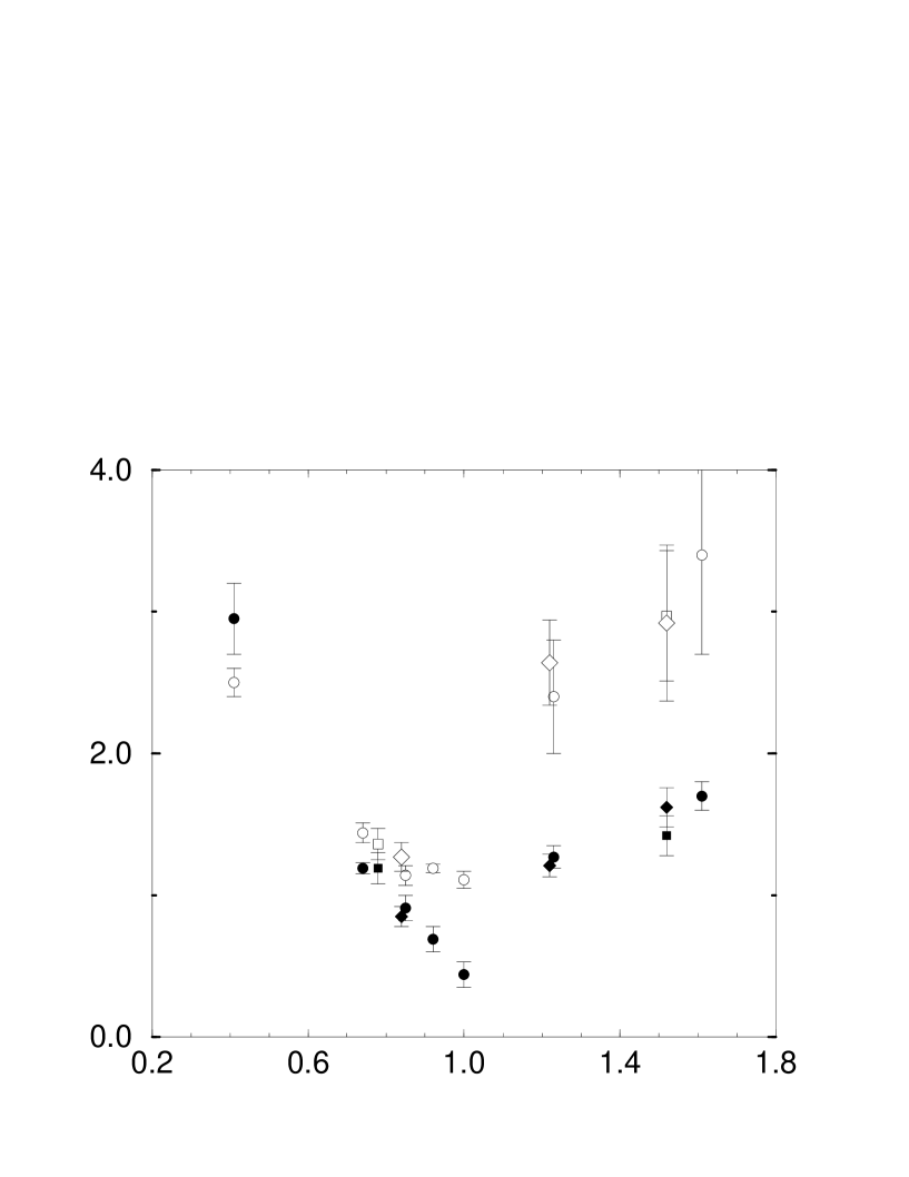
Figure 1: Screening masses $m_{H,W}/g^{2}T$ versus $T/T_{c}$. Solid symbols correspond to $H$, open symbols to $W$; circle: $24^{3}$ data; diamond: $20^{3}$ data; square: $32^{3}$ data.

Table 3 also shows the results for the screening masses of these additional simulations. We fitted the data at $d=3$ – 5 for $N=20$ and at $d=4$ – 7 for $N=32$. Fig. 1 shows the screening masses in physical units, $m/g^{2}T$, versus $T/T_{c}$. The transition at $T=T_{c}$ is clearly visible and we also see the ratio $m_{H}/m_{W}$ approaching 1 at low temperatures, as expected from the choice $\bar{\lambda}=1/2$. (The dimensional reduction approximation is of course questionable at the most left points where $T/M_{H}$ is only 0.88.) We observe no significant volume dependence away from the phase transition in the data at $T/T_{c}=0.85$ and 1.23. The data at $T/T_{c}=1.52$ ($20^{3}$, $\bar{\beta}=11^{*}$ and $32^{3}$, 18.3) show reasonable lattice spacing independence (recall that the ratio of lattice spacings is 0.6). The difference in $m/g^{2}T$ between $\bar{\beta}=13^{\prime}$ ($20^{3}$) and 21.7 ($32^{3}$) is evidently due to the difference in physical temperatures, $T/T_{c}=0.84$ and 0.78, and not a signal of lattice spacing dependence.

$\bar{\beta}$ $am_{{\rm eff}\,H}$ $am_{{\rm eff}\,W}$ $m_{{\rm eff}\,H}/g^{2}T$ $m_{{\rm eff}\,W}/g^{2}T$ $13^{\prime}$ 0.24(2) 0.43(4) 0.78(7) 1.40(13) 21.7 0.18(3) 0.27(3) 0.98(16) 1.46(16) $11^{\prime}$ 0.64(5) 1.65(14) 1.76(14) 4.5(4) $11^{\ast}$ 0.64(4) 1.84(13) 1.76(11) 5.1(4) 18.3 0.32(5) 1.26(11) 1.46(23) 5.8(5)

Table 4: Effective screening masses from eq. (22).

We also like to mention our experience with a momentum space analysis of the correlation functions, which has been popular in numerical studies of the Higgs-Yukawa sector of the Standard Model. This analysis is based on the Fourier transform of $G_{H,W}(d)$,

$$G_{H,W}(p)=\sum_{d}e^{-ipd}\,G_{H,W}(d).$$ (21)

Here $p$ is one of the lattice momenta, $ap=2\pi n/N$, $n=0,1,\cdots,N-1$. Within statistical errors these are real functions of $p$. We deduced effective screening masses $m_{\rm eff}$ from the expansion

$$G(p)^{-1}=Z^{-1}[a^{2}m_{\rm eff}^{2}+p^{2}+O(p^{4})],$$ (22)

by fitting $G^{-1}$ as a function of $\hat{p}^{2}\equiv 2-2\cos ap$ to a straight line, using two of the lower $p$ values ($n=ap/(2\pi/N)=0,1$ and 1,2). The resulting effective screening masses (cf. Table 4) tend to be significantly larger than the true screening masses above, especially for $W$ in the plasma phase, for which $G^{-1}(p)$ shows strong curvature. (Fitting more data points to a quadratic function had no significant effect on the results.) The effective masses are expected to be a good approximation to the screening masses only in case of pole dominance of $G(p)$, which evidently is not the case for $W$ in the plasma phase.

It is known that in the Higgs phase the simple fields (15, 16) which we use perform reasonably well in creating dominantly the $H$ and $W$ out of the vacuum, but in the plasma phase they easily create also excited states with the same quantum numbers as $H$ and $W$ (for a recent study see [28]). The excited state contribution weakens of course pole dominance. To do better one has to use more sophisticated observables instead of the simple $H_{{\bf x}}$ and $W_{k{\bf x}}^{\alpha}$, e.g. the smeared fields used in [28].

5 Plasmon correlators in the Higgs phase

The results in the previous section for the screening properties of $H$ and $W$ give us a feeling how well we are doing in a familiar situation, in the theoretical framework of dimensional reduction. We now turn to the time dependent correlation functions, for which we are on less established ground. Figs. 2 and 3 show an initial scan of the autocorrelation functions $C_{H}(t)$ and $C_{W}(t)$ for various $\bar{\beta}$ at fixed $\bar{v}^{2}=\bar{v}^{2}_{c}(\bar{\beta}=12)$ on the $24^{3}$ lattice. The horizontal time scale is in lattice units (i.e.  (number of time integration steps) $\times$ (step size) as it appears in the computer code). The time in lattice units can be converted to physical units by multiplication with e.g. the temperature in lattice units. We see the period of the oscillations increasing as we approach the transition at $\bar{\beta}=12$ from above (from the Higgs side).

In the $H$ case (Fig. 2) there is a drastic change of behavior below $\bar{\beta}=12$ (the plasma side), where the signal is much smaller. As the insert shows the data here is very noisy, although we think the very short time ($t<2$) data is still relevant, because short times allow for more microcanonical averaging. Notice the oscillations in this very short time region.

For $W$ (Fig. 3) the transition appears more gradual. As $\bar{\beta}$ is lowered down from 20, small oscillations in the small time region ($t<2$) appear already in the Higgs phase. When $\bar{\beta}$ is decreased further below 12 the initial oscillations increase somewhat and so does the slope afterwards, which is nearly zero for $\bar{\beta}=11$, 10, 8. In this case we have stopped the drawing of the curves at early times because the statistical noise would be overwhelming.

To extract a plasmon frequency and damping rate we fit the data in the Higgs phase to the simple asymptotic form

$$Re^{-\gamma t}\cos(\omega t+\alpha)+C.$$ (23)

For a free scalar field we would have $R=T/m^{2}$, $\gamma=C=0$. With interactions the form (23) is expected to be a good approximation in case of small damping [36]. It turns out that the phase $\alpha$ is not really needed and may be set equal to zero. In the plasma phase the signal of our $24^{3}$ data is too noisy for a quantitative analysis. For the Higgs phase the $24^{3}$ data led to the plasmon parameters shown in Tables 5 and 6. The errors are based on jackknifing with respect to the initial conditions. The damping rate $\gamma$ is sensitive to the beginning of the fitting range, the fits above started roughly from the third maximum of $C_{H}(t)$ (the first maximum is at $t=0$).

$\bar{\beta}$ $N$ $T/T_{c}$ $a\omega_{H}$ $a\omega_{W}$ $\omega_{H}/g^{2}T$ $\omega_{W}/g^{2}T$ 20 24 0.41 0.508(2) 0.551(2) 2.54(1) 2.76(1) 14 24 0.74 0.350(4) 0.430(6) 1.23(2) 1.51(2) 21.7 32 0.78 0.210(2) 0.296(2) 1.14(1) 1.61(1) 13 24 0.85 0.28(2) 0.38(2) 0.91(7) 1.24(7) $13^{\prime}$ 20 0.85 0.284(5) 0.382(5) 0.92(2) 1.24(2) 12.5 24 0.92 0.24(1) 0.35(2) 0.75(3) 1.09(6) 12 24 1 0.16(1) — 0.48(3) — $11^{\prime}$ 20 1.23 0.33(3) — 0.91(8) — $11^{\ast}$ 20 1.52 0.44(3) — 1.21(8) — 18.3 32 1.52 0.23(2) — 1.05(9) —

Table 5: Results for the plasmon frequencies.

$\bar{\beta}$ $N$ $T/T_{c}$ $a\gamma_{H}$ $a\gamma_{W}$ $\gamma_{H}/g^{2}T$ $\gamma_{W}/g^{2}T$ 20 24 0.41 0.0012(19) 0.008(4) 0.006(10) 0.04(2) 14 24 0.74 0.0045(31) 0.03(1) 0.016(11) 0.105(35) 21.7 32 0.78 0.0052(8) 0.041(8) 0.028(4) 0.22(4) 13 24 0.85 0.013(29) 0.04(5) 0.042(94) 0.13(16) $13^{\prime}$ 20 0.85 0.011(5) 0.08(2) 0.036(16) 0.26(7) 12.5 24 0.92 0.012(8) 0.09(9) 0.038(25) 0.28(28) 12 24 1 0.03(2) – 0.09(6) — $11^{\prime}$ 20 1.23 0.079(61) 0.0116(17) 0.22(17) 0.032(5) $11^{\ast}$ 20 1.52 0.053(55) 0.0111(6) 0.15(15) 0.031(2) 18.3 32 1.52 0.036(40) 0.0062(8) 0.16(18) 0.028(4)

Table 6: Results for the damping rates.

We increased the numerical effort on the plasma phase parameters values $\bar{\beta}=11^{\prime}$, $11^{*}$ and 18.3 and did similar runs for $13^{\prime}$ and 21.7. Fig. 4 shows the autocorrelation function $C_{H}(t)$ in the Higgs phase for $\bar{\beta}=13^{\prime}$ and 21.7. A fit to (23) starting roughly at the third maximum led to the plasmon parameters shown in Tables 5 and 6. Figure 5 shows the $W$-autocorrelation functions in the Higgs phase. It is clear that the $W$ damping rate is considerably larger than for $H$ and to avoid running into noise we had to lower the starting time of the fit to (23) down to roughly the second maximum. The constant $C$ of the fits is non-zero. However, we have seen the autocorrelators to tend to zero at very large times. The results in physical units are shown in Figs. 6 and 7. From the smooth adjustment of the $\bar{\beta}=21.7$ ($32^{3}$) data with the $\bar{\beta}=13^{\prime}$ and 13 ($20^{3}$ and $24^{3}$) data it follows that the plasmon frequencies and damping rates are nearly lattice spacing independent.

However, the $32^{3}$ data point in Fig. 6 for the $W$ plasmon frequency at $T/T_{c}=0.78$ does look somewhat high compared to the trend of the $24^{3}$ data. Interpolating the $24^{3}$ data linearly between $T/T_{c}=0.74$ and 0.85 gives us a hypothetical data point $\omega_{W}/g^{2}T=1.41(3)$ at $T/T_{c}=0.78$, $\bar{\beta}=13.6$. The $32^{3}$ data point at $T/T_{c}=0.78$, 1.61(1), is a factor 1.14 higher. This is much less than the corresponding ratio of lattice spacings, 21.7/13.6 = 1.60, and in the previous version of this paper we ignored this 14% discrepancy as due to a possible systematic error in our data analysis. Now we shall take it seriously and try to interpret it as an expression of lattice spacing dependence. As a rough model, let us assume that $\omega_{H}^{2}=2\lambda v^{2}$, $\omega_{W}^{2}=g^{2}v^{2}/4+\tilde{\omega}^{2}$, where $v^{2}$ is simply defined by the equation $v^{2}=\omega_{H}^{2}/2\lambda$, and $\tilde{\omega}^{2}$ is an additional contribution to the $W$-plasmon frequency. Since the Higgs parameters are tuned according to dimensional reduction we assume that $\omega_{H}^{2}$ is independent of $a$. This is consistent with the trend of the data in Fig. 6. With $\lambda/g^{2}=1/8$ we get $\omega_{W}^{2}=\omega_{H}^{2}+\tilde{\omega}^{2}$. Hard thermal loop arguments [18] lead to the conclusion that there is a divergent component in $\omega_{W}^{2}$, given by $0.08606C_{A}g^{2}T/a$, with $C_{A}=2$ for SU(2). We have checked in a one loop calculation perturbative calculation on the lattice that a scalar gives the same with $C_{A}\to 1/2$. Let us now assume $\tilde{\omega}^{2}$ to be this divergent contribution, and write $\tilde{\omega}^{2}=\delta g^{2}T/a$. Then $\delta=(2+1/2)\,0.08606=0.2151$. Denoting the interpolated $\bar{\beta}=13.6$ data by the subscript 1 and the $\bar{\beta}=21.7$ data without a subscript, we have with $\omega_{H}/g^{2}T=1.14$, $a\omega_{H}=0.210$ (cf Table 5) and $a_{1}\omega_{H}=a\omega_{H}*(a_{1}/a)=0.210*(21.7/13.6)$,

$$\frac{\omega_{W}}{\omega_{1W}}=\sqrt{\frac{\omega_{H}^{2}+\tilde{\omega}^{2}}{\omega_{H}^{2}+\tilde{\omega}_{1}^{2}}}=\sqrt{\frac{1+\delta(g^{2}T/\omega_{H})/(a\omega_{H})}{1+\delta(g^{2}T/\omega_{H})/(a_{1}\omega_{H})}}=\sqrt{\frac{1+4.18\,\delta}{1+2.62\,\delta}}=1.10,$$ (24)

for $\delta=0.2151$. This is somewhat smaller than the ‘measured’ ratio $\omega_{W}/\omega_{1W}=1.61/1.41=1.14$. Using this as input and solving for $\delta$ would give $\delta=0.38$. Notice that the $\delta$-terms in the last square root above are not small compared to one. In this interpretation all the difference between $\omega_{H}$ and $\omega_{W}$ is ascribed to the $\delta$-contribution, which is probably not the whole story in a more detailed perturbative calculation, but which works reasonably well. For example, $\omega_{W}/\omega_{H}-1=0.41$ for the 21.7 data, while $\sqrt{1+4.18\,\delta}-1=0.38$ for $\delta=0.2151$. Furthermore, for $\bar{\beta}=12.5$, 13, 14, 20 the predicition for $\omega_{W}/\omega_{H}-1$ is 0.48, 0.36, 0.22, 0.080, respectively, to be compared with the data 0.46, 0.36, 0.23, 0.085. The above interpretation suggests that the approximate lattice spacing independence of our data for the plasmon frequencies is fortuitous and that it may well turn into a clear $1/\sqrt{a}$ behavior at much smaller lattice spacings.

6 Autocorrelators in the plasma phase

In the plasma phase the behavior is qualitatively different. Fig. 8 shows that $C_{H}(t)$ still has roughly the form (23), but with an average $C$ that gets significantly smaller in a period of oscillation. A reasonable fit to the data could be obtained by letting $C\to Ct^{-\delta}$ in a region starting a little before the second maximum to times where the oscillations appear to have died out, judging by eye. An example of such a fit is shown in figure 8. The large statistical errors for $C_{H}$ in the Higgs phase show up in the lack of smoothness in the data and the resulting jackknife error on $\gamma_{H}$ is very large. The results are in Tables 5, 6 and Figs. 6 and 7. The fitted power $\delta$ is about 0.2 – 0.4. For larger times ($t>100$ for $11^{*}$) the power $\delta$ appears to increase, as shown in the double logarithmic plot Fig. 9, which also shows that there is no good evidence for exponential behavior. Asymptotically one would expect the $t^{-3/2}$ behavior familiar from zero temperature [36].

The $W$ autocorrelator behaves very differently. Fig. 10 shows what looks like $C_{H}(t)$ in Fig. 8, except that the time scale has shrunk by an order of magnitude. The periods of the oscillations are of order 1, which suggests $\omega$’s of order $2\pi$ and also the $\gamma$’s appear to be very large in lattice units. There is clearly no scaling in this time interval since the period of the oscillation hardly changes as $\bar{\beta}$ increases. We recall that the oscillations start already in the Higgs phase quite far from the phase transition, as mentioned above after introducing Fig. 3. They are not analogous to those of $C_{H}(t)$ in Fig. 8, but of $C_{H}(t)$ in the insert in Fig. 2. The small time oscillations correspond to energies of the order of the cutoff and must be considered as dominated by lattice artefacts.

Fig. 11 shows the larger time region on a logarithmic scale. We see good evidence for exponential behavior. A power behavior appears to be excluded in the time range shown (cf. insert). The drop of $C_{W}(t)$ can be fitted to an exponential with a damping rate in physical units that is lattice spacing independent, within errors, as shown in Table 6 and Fig. 6. On the other hand, the slopes of $\bar{\beta}=11^{\prime}$ and $11^{\ast}$ are equal within errors which suggests that the $W$ dynamics is practically independent of the scalar field dynamics in the plasma phase. A similar effect has been noticed for the screening lengths, see e.g. [28]. There appear to be no oscillations in the exponential regime. At very large times we found irregular oscillations with a period of order 600 (18.3 data), indicating a frequency of order 0.01, but the statistics is insufficient to be able to say anything more definite.

Ignoring this hint of oscillations at large times as being noise, it is interesting to explore an interpretation in terms of overdamping such as discussed in [16, 18]. Suppose the $W$ mode satisfies an equation of the form $(\partial_{t}^{2}+\Gamma\partial_{t}+M^{2})C_{W}(t)=0$ for $t>0$, with some basic frequency $M$ and damping rate $\Gamma$. Substituting $\exp(-i\omega t)$ gives the equation $-\omega^{2}-i\Gamma\omega+M^{2}=0$. For small $\Gamma^{2}\ll M^{2}$ this leads to damped oscillations, but for large $\Gamma^{2}\gg M^{2}$ the system is overdamped, in the sense that the solutions $\omega$ are purely imaginary and no oscillations occur: $\omega_{1}\approx-i\Gamma$, $\omega_{2}\approx-iM^{2}/\Gamma$. Identifying the smaller $|\omega_{2}|$ with our measured damping rate $\gamma_{W}$, we can try to interpret $C_{W}(t)$ for $\bar{\beta}=18.3$ with $a\Gamma=O(0.5)$ (qualitatively representing the strong damping in Fig. 10, while ignoring the oscillations) and $aM=a\sqrt{\gamma_{W}\Gamma}=\sqrt{0.0062\,a\Gamma}=O(0.06)$. However, since the above equation for $C_{W}(t)$ is supposed to hold under the condition $|\omega|^{2}\ll M^{2}$, it seems best to discard $\omega_{1}$ altogether. It is interesting that $\gamma_{W}$ is inversely proportional to $\Gamma$.

7 Discussion

We have learned that numerical computations of real time correlation functions in hot SU(2)-Higgs theory are feasible in the classical approximation. In this exploratory study we have not indicated statistical errors in our plots of the correlation functions. In most cases these are quite reasonable, but in some they would swamp the data lines, e.g. for $H$ in the plasma phase. However, we believe the jackknife errors given in Tables 5, 6 and Figs. 6, 7 are mostly realistic and they can be improved with a reasonable increase of computational effort. The errors on $\gamma_{H}$ appear to be overestimated, but this can only be clarified by increasing statistics. Systematic errors are harder to assess. It is one thing to compute an autocorrelation function, and quite another to extract plasmon parameters from these when the damping rate is relatively large. But then the very relevance of such concepts is questionable in case of strong damping.

The results for the $H,W$ plasmon frequencies and damping rates appear to be roughly independent of the lattice spacing $a$. We found, however, that a small effect in the $W$ frequency at $T/T_{c}=0.78$ could be interpreted as compatible with the expected $1/\sqrt{a}$ divergence [18]. The approximate $a$-independence of the $H$ frequency may due to the fact that Higgs screening mass is already tuned by the counterterms based on dimensional reduction (for the $W$ there is no room for such tuning within the classical form of the hamiltonian).

As argued in the Introduction, comparison with analytical results in the quantum theory is to be done in the Higgs phase. The numerical damping rates in the Higgs phase compare reasonably well: the $\bar{\beta}=21.7$ ($T/T_{c}=0.78$) data give $\gamma_{W}/g^{2}T=0.22(4)$ and $\gamma_{H}/g^{2}T=0.028(4)$, to be compared with $0.176$ and $\approx 0.02$, respectively [37, 38]. Of course, these values will depend on the distance from the transition at $T_{c}$ (cf. Fig. 6). The approximate lattice spacing independence of the damping rates may express an insensitivity to the magnitude of the plasmon frequency. This is the case in the quantum theory where the plasmon frequency is of order $gT$ and the damping rate of order $g^{2}T$, which is the primary scale of the classical theory. We note also that the perturbative values for the quantum and classical plasmon frequencies for the gauge field are in fact not very different in our simulation: for SU(2) gauge theory we have $a\omega_{W}^{\rm qu}=2\sqrt{2}/\bar{\beta}$ and $a\omega_{W}^{\rm cl}=0.8297/\sqrt{\bar{\beta}}$ [18], which are equal for $\bar{\beta}=11.6$.

The damping rate associated with $H$ increases substantially when the temperature is raised above $T_{c}$, while the rate associated with $W$ drops dramatically. Both damping rates appear to be roughly temperature independent in the plasma phase, although the errors on $\gamma_{H}$ are much too large for a definite conclusion. The data for the $W$ correlation function in the plasma phase suggest overdamping, with a rather small damping rate. For a proper interpretation we may have to do better than just a pole approximation to the correlation function. It is interesting that a similar phenomenon was found recently in a simulation of correlators of SU(2) gauge fields, transformed to Coulomb gauge [14]. We stress again that in the plasma phase the ‘plasmon’ frequencies and damping rates of the composite $H$ and $W$ fields should not be identified with those of the elementary Higgs and gauge fields.

Acknowledgement
The numerical simulations made use of the code [33] kindly provided to us by Alex Krasnitz. We thank Gert Aarts, Peter Arnold and Alex Krasnitz for useful remarks. This work is supported by FOM and NCF, with financial support from NWO.

Figure 2: Scan of $C_{H}(t)$ from the $24^{3}$ data. The first minima in $t>5$ are in order of decreasing $\bar{\beta}=20$, 14, 13, 12.5, 12. The lines in the middle of the $C_{H}$ plot are for $\bar{\beta}<12$, shown enlarged in the insert.

Figure 3: Scan of $C_{W}(t)$ from the $24^{3}$ data. The first minima in $t>5$ are in order of decreasing $\bar{\beta}=20$, 14, 13, 12.5, 12. The lines ending before $t=10$ are for $\bar{\beta}<12$; bottom to top ($t=4$): $\bar{\beta}=11$ (touching the minimum of $\bar{\beta}=12$), 10 (nearly coinciding with 11), 8, 6 and 4.

Figure 4: The autocorrelator $C_{H}(t)$ in the Higgs phase for $\bar{\beta}=13^{\prime}$ (small amplitude) and 21.7 (large amplitude).

Figure 5: The autocorrelator $C_{W}(t)$ in the Higgs phase for $\bar{\beta}=13^{\prime}$ (lower tail) and 21.7 (upper tail).

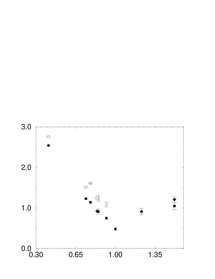
Figure 6: Plasmon frequencies $\omega/g^{2}T$ versus $T/T_{c}$. Solid symbols correspond to $H$, open symbols to $W$; circle: $24^{3}$ data; diamond: $20^{3}$ data; square: $32^{3}$ data.

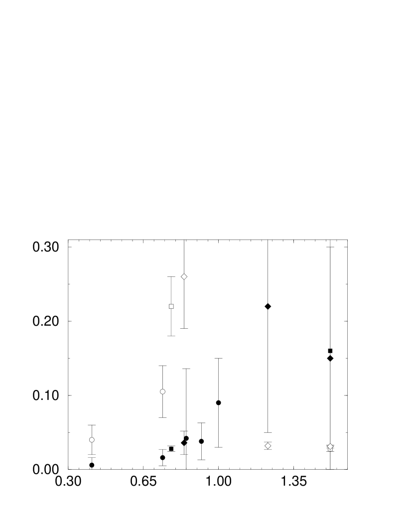
Figure 7: Damping rates $\gamma/g^{2}T$ versus $T/T_{c}$. Solid symbols correspond to $H$, open symbols to $W$; circle: $24^{3}$ data; diamond: $20^{3}$ data; square: $32^{3}$ data.

Figure 8: Left: $C_{H}(t)$ in the plasma phase; $\bar{\beta}=18.3$, $11^{\ast}$ and $11^{\prime}$ in ascending order. Right: fit (dashed curve) to the data at $\bar{\beta}=18.3$; the fitting region corresponds to the data shown.

Figure 9: $\ln C_{H}(t)$ versus $t$ (left) and $\ln C_{H}(t)$ versus $\ln t$ (right) in the plasma phase.

Figure 10: Short time behavior of $C_{W}(t)$ in the plasma phase. Top to bottom ($t\approx 1$): $\bar{\beta}=11^{\prime}$, $11^{\ast}$ and 18.3.

Figure 11: Plot of $\ln C_{W}(t)$ in the plasma phase for larger times; $\bar{\beta}=11^{\prime}$ (top), $11^{\ast}$ (middle) and 18.3 (bottom). The insert shows the same time interval on a double logarithmic plot.

References

- [1] D.Yu. Grigoriev and V.A. Rubakov, Nucl. Phys. B299 (1988) 67.
- [2] D.Yu. Grigoriev and V.A. Rubakov and M.E. Shaposhnikov, Nucl. Phys. B326 (1989) 737.
- [3] A. Bochkarev and P. de Forcrand, Phys. Rev. D47 (1993) 3476.
- [4] A. Krasnitz and R. Potting, Nucl. Phys. B (Proc. Suppl.) 34 (1994) 613.
- [5] J. Smit and W.H. Tang, Nucl. Phys. B (Proc. Suppl.) 34 (1994) 616.
- [6] P. de Forcrand, A. Krasnitz and R. Potting, Phys. Rev. D50 (1994) 6054.
- [7] J. Smit and W.H. Tang, Nucl. Phys. B (Proc. Suppl.) 42 (1995) 590.
- [8] J. Ambjørn, T. Askgaard, H. Porter and M.E. Shaposhnikov, Phys. Lett. B244 (1990) 479; Nucl. Phys. B353 (1991) 346.
- [9] A. Krasnitz, private communication.
- [10] J. Smit and W.H. Tang, Nucl. Phys. B482 (1996) 265.
- [11] J. Ambjørn and A. Krasnitz, Phys. Lett. B362 (1995) 97.
- [12] N. Turok and G. D. Moore, hep-ph/9608350.
- [13] G.D. Moore and N.G. Turok, hep-ph/9703266.
- [14] J. Ambjørn and A. Krasnitz, hep-ph/9705380.
- [15] G.D. Moore, hep-ph/9705248.
- [16] P. Arnold, D. Son and L.G. Yaffe, Phys. Rev. D55 (1997) 6264.
- [17] D. Bödeker, L. Mc Lerran an A. Smilga, Phys. Rev. D52 (1995) 4675.
- [18] P. Arnold, Phys. Rev. D55 (1997) 7781.
- [19] K. Kajantie, M. Laine, K. Rummukainen and M. Shaposhnikov, Nucl. Phys. B458 (1996) 90.
- [20] G. Aarts and J. Smit, Phys. Lett. B393 (1997) 395.
- [21] G. Aarts and J. Smit, hep-ph/9707342.
- [22] C. Hu and B. Müller, hep-ph/9611292.
- [23] V.P. Nair, Phys. Rev. D50 (1994) 4201.
- [24] W. Buchmüller and O. Philipsen, Nucl. Phys. B443 (1995) 47.
- [25] Z. Fodor, J. Hein, K. Jansen, A. Jaster and I. Montvay, Nucl. Phys. B439 (1995) 147.
- [26] M. Gürtler, E.-M. Ilgenfritz, J. Kripfganz, H. Perlt and A. Schiller, Nucl. Phys. B483 (1997) 383.
- [27] K. Kajantie, M. Laine, K. Rummukainen and M. Shaposhnikov, Nucl. Phys. B466 (1996) 189.
- [28] O. Philipsen, M. Teper and H. Wittig, Nucl. Phys. B469 (1996) 445.
- [29] F. Karsch, T. Neuhaus, A. Patkós and J. Rank, Nucl. Phys. B474 (1996) 217.
- [30] K. Jansen, Nucl. Phys. B (Proc. Suppl.) 47 (1996) 196.
- [31] K. Rummukainen, Nucl. Phys. B (Proc. Suppl.) 53 (1997) 30.
- [32] W. Buchmüller and O. Philipsen, Phys. Lett. B397 (1997) 112.
- [33] A. Krasnitz, Nucl. Phys. B455 (1995) 320.
- [34] K. Farakos, K. Kajantie, K. Rummukainen and M. Shaposhnikov, Phys. Lett. B336 (1994) 494.
- [35] K. Kajantie, M. Laine, K. Rummukainen and M. Shaposhnikov, Nucl. Phys. B466 (1996) 189.
- [36] D. Boyanovsky, M. D’Attanasio, H.J. de Vega, R. Holman and D.-S. Lee, Phys. Rev. D52 (1995) 6805.
- [37] E. Braaten and R.D. Pisarski, Phys. Rev. D42 (1990) 2156.
- [38] T.S. Biró and M.H. Thoma, Phys. Rev. D54 (1996) 3465.