Abstract

We investigate SU(2) lattice gauge theory in four dimensions in the maximally abelian projection. Studying the effects on different lattice sizes we show that the deconfinement transition of the fields and the percolation transition of the monopole currents in the three space dimensions are precisely related. To arrive properly at this result the uses of a mathematically sound characterization of the occurring networks of monopole currents and of an appropriate method of gauge fixing turn out to be crucial. In addition we investigate detailed features of the monopole structure in time direction.

1. Introduction

For the conjecture [1, 2] that condensing magnetic monopoles describe quark confinement nonperturbative support first came from compact U(1) lattice gauge theory [3, 4]. To treat the nonabelian case ’t Hooft [5] proposed to extract the relevant abelian degrees in SU(N) gauge theory by a suitable gauge fixing procedure called abelian projection. A nonperturbative realization of this concept has become possible on the lattice [6]. Among the possible choices of such projections the maximally abelian projection [7] appears most appropriate and has been considered in numerous papers [8].

To confirm this picture in Monte Carlo simulations it is attractive not only to measure observables but to analyze the configurations and to look for the structures of monopole currents which are characteristic for the phases and thus are able to signal the deconfinement transition. First analyses of this type have already been presented some time ago [9, 10]. A consideration of the connection of two points by currents [11] is also in this spirit. Analyses of the sizes of the structures have been given in [12, 13]. More recently a quantity called “wrapping number” by the author [14] has been used in the deconfinement phase.

Monopole currents which (on lattices with periodic boundary conditions) wrap around the torus have been typically observed in the confining phase. However, as soon as one goes into more detail and tries to make the characterization precise, the problem becomes obvious that one has to deal with complicated networks of monopole currents rather than with simple loops, for which the topological characterization would be straightforward. Decomposing the networks into loops, apart from being highly ambiguous, is not allowed because it changes the topology.

In the context of the deconfinement transition this problem so far has not been addressed. In [14] it has been noted that the considerations there could not be extended to the confining phase because of the occurrence of entangled structures rather than of simple loops. Otherwise the indicated problem so far has not been mentioned in the respective literature.

In U(1) gauge theory in four dimensions the related problem has recently been solved using mappings which preserve homotopy [15, 16]. This has lead to an unambiguous characterization of the phases by the presence or absence of a current network which is topologically nontrival in all directions. More generally this means presence or absence of an infinite network where the definition of “infinite” on the finite lattice is dictated by the boundary conditions [17]. For periodic boundary conditions it has been checked in detail that neither size nor extension but precisely the topological properties are the crucial ones.

These results suggest to try an analogous characterization of the deconfinement transition. In that case the percolation phenomenon of the monopole currents should occur only in the three space directions. Due to the fact that the characterization is by the indicated topological properties there is no problem giving a consistent prescription also in the three-dimensional subspace.

Within the latter respect a conceptual problem exists for the other quantities considered so far, i.e. for monopole density [9, 12], sizes of monopole loops [12, 13] and quantities related to cluster size [10]. We have checked, using larger lattices and higher statistics, that such quantities also empirically do not lead to a convincing characterization.

The indicated characterization by the topology of networks has the advantage that it is insensitive to short range fluctuations. In fact, as has been shown in the case of U(1) gauge theory [15, 16, 17], and as turns out also here, it is solely sensitive to the percolation phenomenon, i.e. to extreme long distance properties. In practice the characteristic probability for the occurrence of a network which is nontrivial in the three space directions, taking sharp values 0 and 1, allows determination of the phases at very low computational cost.

In addition to showing that the topological properties signal the percolation transition it is to be checked wether its transition point coincides with that of the deconfining transition of the fields. This is important because there are examples where there is no such coincidence [18, 19, 20]. In the only work [10] in which percolation is discussed in the context of the deconfinement transition, the coincidence of the respective transition points is considered to be an open question.

It has been observed in Ref. [10] that loops of monopole currents being nontrivial in the time direction survive in the deconfinement phase. Such loops have also been studied in Ref. [14] by using the concept of a “wrapping number”. This quantity has already been introduced in [21]. It has been shown, because of current conservation, to equal the net current flow [15]. In U(1) gauge theory it is known to fail to characterize the transition [21, 15]. Thus it appears desirable to investigate in more detail what happens in time direction which, as mentioned above, should not be involved in the percolation.

A further question is wether the nontrivial loops in time direction are really simple loops and not, in general, networks with a similar number of contacts (crossings of monopole currents) as have been observed in U(1) theory. The mean numbers per volume of contacts there turn out to be rather insensitive to sizes of lattices and of monopole structures [15], which indicates a rather uniform density of the contacts within the monopole structures. Thus it should be clarified wether the same phemomenon occurs also here.

In the present letter we consider SU(2) gauge theory in the maximally abelian projection putting particular effort on careful gauge fixing. We apply the method of analyzing networks of monopole currents developed before in U(1) gauge theory [15, 16] and show that the percolation transition of the monopole currents in the three space dimensions precisely coincides with the deconfinement transition of the fields. In addition we investigate detailed features of the structure of the monopole currents in time direction.

2. Gauge fixing

The maximally abelian gauge [7] is obtained by performing gauge transformations which maximize the quantity

$$R=\sum_{x,\mu}Tr(\sigma_{3}U_{\mu,x}\sigma_{3}U^{\dagger}_{\mu,x})\quad.$$ (2.1)

The conventional procedure is to perform local gauge transformations iteratively throughout the lattice until sufficient accuracy is reached. By introducing an overrelaxation parameter $\omega$ [22] the efficiency of this method can be considerably improved [23]. For this either the fixed choice $\omega=1.7$ [24] or choosing stochastically [25] $\omega=1$ (no overrelaxation) in 10% of cases and $\omega=2$ otherwise has turned out to be advantageous.

Applying the overrelaxation methods one may still get stuck at some local maximum of (2.1). A method suitable to reach the global maximum is simulated annealing [26]. We find that for the present purpose to use such a technique is indeed crucial. The necessity of using simulated annealing has recently also been pointed out in the context of abelian potentials [27].

Our procedure for simulated annealing uses Metropolis sweeps based on a probability distribution $P(R)\sim\exp(\alpha R)$ in which changes of R by random local gauge transformations are proposed. After an appropriate number of sweeps at each $\alpha$ the value of $\alpha$ has been increased by a suitable amount and the simulations continued at the new value. After the simulated annealing steps in addition an overrelaxation algorithm has been applied. Thus essentially first annealing finds the proper maximum and then overrelaxation quickly determines the precise numerical value of its location.

To have some control of the quality of the procedure we have always applied it to several gauge copies (created by random gauge transformations of one configuration). We then have considered the data separately for the best, the first and the worst copy. By varying the quality of the procedure we have checked that it is appropriate to associate “best” to the largest value of $R$ and “worst” to the smallest one.

In standard runs we used 20 $\alpha$ values and 10 sweeps at each of them for annealing. We stopped the overelaxation steps after $Z=10^{-7}$ has been reached, where $Z$ is given by [23]

$$Z=\frac{1}{L^{4}}\sum_{x}[(X_{x}^{1})^{2}+(X_{x}^{2})^{2}]\quad,$$ (2.2)

with $X_{x}=\sum_{\mu}(U_{\mu,x}\sigma_{3}U^{\dagger}_{\mu,x}+U^{\dagger}_{\mu,x-\mu}\sigma_{3}U_{\mu,x-\mu})$ , and considered 4 gauge copies. To check the reliability of the standard run choices we performed high quality runs with 600 $\alpha$-values and 100 sweeps at each of them for annealing. Only minor deviations from the best copy results of the standard runs have been observed. These deviations have remained within the statistical errors of the measured quantities.

3. Topological analysis

In the maximally abelian gauge the coset decomposition of SU(2) with respect to the Cartan subgroup U(1) is $U_{\mu,x}=w_{\mu,x}u_{\mu,x}$ with $tr(w_{\mu,x}\sigma_{3})=0$ and where $u_{\mu,x}=\exp(i\theta_{\mu,x}\sigma_{3})$ is diagonal. The abelian physical flux $\bar{\theta}_{\mu\nu,x}$ is given by $\theta_{\mu\nu,x}=\bar{\theta}_{\mu\nu,x}+2\pi n_{\mu\nu,x}$ with $n_{\mu\nu,x}=0,\pm 1,\pm 2$ and $\bar{\theta}_{\mu\nu,x}\in[-\pi,\pi)$ [4]. Defining the monopole currents related to the links of the dual lattice by

$$J_{\mu,x}=\frac{1}{2\pi}\epsilon_{\mu\nu\sigma\rho}(\bar{\theta}_{\sigma\rho,x+\mu+\nu}-\bar{\theta}_{\sigma\rho,x+\mu})$$ (3.1)

the conservation law

$$\sum_{\mu}(J_{\mu,x}-J_{\mu,x-\mu})=0$$ (3.2)

has the simple geometrical meaning that incoming and outgoing currents compensate at each site of the dual lattice.

We define current lines in terms of the currents as follows: for $J_{\mu,x}=0$ there is no line on the link, for $J_{\mu,x}=\pm 1$ there is one line, and for $J_{\mu,x}=\pm 2$ there are two lines, in positive or negative direction, respectively. Networks of currents are connected sets of current lines. For a network N disconnected from the rest the net current flow $\vec{f}$ has the components

$$f_{\mu_{3}}=\sum_{x_{\mu_{0}}x_{\mu_{1}}x_{\mu_{2}}}J_{\mu_{3},x}\quad\mbox{for}\quad J_{\mu,x}\in\mbox{{\bf N}}\quad.$$ (3.3)

By (3.2) the net current flows of the occurring networks have to sum up to zero.

The topological characterization of networks is based on the following observation. The elements of the fundamental homotopy group are equivalence classes of paths starting and ending at a base point $b$ which can be deformed continuously into each other. The generators of the group may be obtained embedding a sufficiently dense network N into its space X and performing suitable transformations which preserve homotopy. If a given network N does not wrap around in all directions, then only the generators of a subgroup are produced. This fact can be utilized for an unambiguous characterization of networks.

In practice we choose one vertex point of N to be the base point $b$ and consider all paths which start and end at $b$. A mapping which shrinks one edge to zero length preserves the homotopy of all of these paths. Therefore, by a sequence of such mappings we can shift all other vertices to $b$ without changing the group content until we finally obtain a bouquet of paths which all start and end at $b$. In this procedure we describe a path by a vector which is the sum of oriented steps along the path. The bouquet vectors then form a matrix which is to be analyzed with respect to its generator content. This is achieved by a modified Gauss elimination procedure which respects current conservation.

Thus this analysis, on which more details are given in [15, 16], tells in which directions the network is nontrivial, which are the directions for which generators are found (i.e. for which bouquet loops occur which wrap around the torus).

4. Results

Our Monte Carlo simulations have been performed with the Wilson action on lattices $8^{3}\times 4$, $12^{3}\times 4$ and $18^{3}\times 4$. The measurements with gauge fixing and analysis of configurations have been separated by 100 simulation sweeps. Typically about 100 measurements have been evaluated at each $\beta$-value.

Figure 1 shows the probability $P_{\mbox{\scriptsize net}}$ for the occurrence of a network which is nontrivial in the three space directions as function of $\beta$ which we have obtained on lattices $18^{3}\times 4$, $12^{3}\times 4$ and $8^{3}\times 4$ for best, first and worst gauge copies. The line along the best copy results is drawn to guide the eye. It is seen that as soon as the lattice is large enough one gets a clear signal, $P_{\mbox{\scriptsize net}}$ taking the value 1 in the confining phase and 0 in the deconfining phase. In particular, it turns out that for increasing lattice size the transition point approaches the one determined from Polyakov loop data (where the most recent value is $\beta_{c}=2.29895(10)$ [28]).

From Figure 1 it can also be seen that going from the data of the best copy via the ones of the first copy to those of the worst copy the transition appears to shift slightly to the right. The smallness of this shift shows that the careful gauge fixing described in Sect. 2 is successful. Its direction shows that a shift due to bad gauge fixing would have the same direction as one due to smaller finite size effects on larger lattices. Therefore, reliable gauge fixing is crucial for the present purpose.

With respect to the number of nontrivial networks we find that in the confining phase there is always (in all of our measurements) just one nontrivial network and correspondingly its net current flow is zero. In the deconfinement phase there is no network which is nontrivial in the three space directions.

The percolation phenomenon in three dimensions observed here is seen to be completely analogous to that found in U(1) gauge theory in four dimensions. Similarly as in the U(1) case various alternative possibilities have been checked. It again has turned out that precisely the indicated topological properties are the crucial ones and give a completely consistent description.

Next we consider the structure of the monopole currents in time direction. The probability for finding a current network which is nontrivial in time direction in the $\beta$ range considered is one on lattices $18^{3}\times 4$ and $12^{3}\times 4$ , i.e. in these cases we find always such a network. On the $8^{3}\times 4$ lattice it is one at $\beta=2.2$ and decreases for larger $\beta$ , at $\beta=2.4$ taking a value of about 0.6 for the best gauge copy and of about 0.8 for the worst copy.

Thus it turns out that nontrivial topology in time direction is certain in both phases as soon as the lattice is large enough. Again it becomes obvious that the $8^{3}\times 4$ lattice is too small to produce typical results. From the comparison of best and worst copies it is again seen that worsening gauge fixing causes a change in the same direction as one due to smaller finite size effects on larger lattices. Thus careful gauge fixing is important also here.

A particular feature is that in time direction quite a number of nontrivial networks occur in the deconfinement phase. Figure 2 gives the average numbers per lattice volume of networks being nontrivial in time direction and of simple nontrivial loops in this direction as function of $\beta$ , which we have obtained on lattices $18^{3}\times 4$, $12^{3}\times 4$ and $8^{3}\times 4$ for best gauge copies. Obviously there is little dependence on the lattice size.

From Figure 2 it is seen that though there is some fraction of simple loops in general one has to deal with networks. The observation of a particular fraction at a given value of $\beta$ is related to the observation already made in U(1) lattice gauge theory [15] that the average number of contacts of current lines per size has a definite value which is rather independent of the sizes of the lattice and of the particular current structures.

The number of contacts at a site is defined by the number of lines arriving at the site (or, equivalently, departing from it) minus one. Figure 3a shows the average number of contacts of current lines per size $n_{\mbox{\scriptsize c}}$ as function of $\beta$ for all networks and Figure 3b $n_{\mbox{\scriptsize c}}$ for those nontrivial in time direction. It is seen that for the latter ones one gets only slightly larger values.

Thus the situation is analogous as in U(1) gauge theory where the numbers for larger networks are only slightly larger than the overall ones [15]. The explanation is that the density of contacts gets uniform as soon as the structures are sufficiently extended. To demonstrate this effect in the present context we show in Figure 3c that a slight increase is also observed if the plaquette-like current loops are omitted. It is seen that for the largest lattice then about the same values as in Figure 3b are reached.

The number of contacts turns out to decrease with $\beta$ as one should expect. The numerical value at the transition point is about a factor 1.5 smaller as in U(1) theory, i.e. the numbers $n_{\mbox{\scriptsize c}}$ are of the same order of magnitude. Thus the observed current networks are of the same type.

If there is more than one nontrivial network, nonzero net current flows become possible [15]. In the case under consideration they, in fact, occur. Figure 4 shows the average numbers per volume of networks with net current flows of modulus 0, 1 and 2 in time direction as function of $\beta$ which we have got on lattices $18^{3}\times 4$, $12^{3}\times 4$ and $8^{3}\times 4$ for the best gauge copy. Apparently $|f_{0}|=1$ is most frequent while $|f_{0}|=2$ is relativly rare. Higher values have not been observed. Again it is seen that there is little dependence on the lattice size.

Possibilities to explain the features occurring in the deconfinement phase by ’t Hooft-Polyakov monopoles have been discussed in various papers. The situation has been reviewed by Smit and van der Sijs [29] who have presented detailed analytical investigations. The picture developed by these authors, in fact, predicts nontrivial current loops in time direction to persist in the deconfinement phase. Some caution with this picture, based on classical solutions and dimensional reduction arguments, because of the number of assumptions involved appears, however, appropriate.

A simpler explanation may focus on the fact that the extension in time direction is really very small. Thus, since the current distribution should be sufficiently uniform, one can generally expect easy bridging of the torus by monopole currents in that direction.

Figure captions

Fig. 1.	Probability $P_{\mbox{\scriptsize net}}$ as function of $\beta$
	on lattices $18^{3}\times 4$, $12^{3}\times 4$ and $8^{3}\times 4$
	for best (circles), first (squares) and worst (diamonds) gauge copies.
Fig. 2.	Numbers per volume $n_{\mbox{\scriptsize s}}$ of networks nontrivial in time direction (circles)
	and of simple loops nontrivial in time direction (squares) as function
	of $\beta$ on lattices $18^{3}\times 4$, $12^{3}\times 4$ and $8^{3}\times 4$ for best gauge copy.
Fig. 3.	Average number per size $n_{\mbox{\scriptsize c}}$ of contacts of current lines, (a) for all networks,
	(b) for networks nontrivial in time direction, (c) for networks except
	plaquet-type ones, on lattices $18^{3}\times 4$ (circles), $12^{3}\times 4$ (squares)
	and $8^{3}\times 4$ (diamonds) for best gauge copy.
Fig. 4.	Numbers per volume $n_{\mbox{\scriptsize f}}$ of networks with flows $|f_{0}|=0$ (circles), $|f_{0}|=1$
	(squares) and $|f_{0}|=2$ (diamonds) in time direction as function of $\beta$
	on lattices $18^{3}\times 4$, $12^{3}\times 4$ and $8^{3}\times 4$ for best gauge copy.

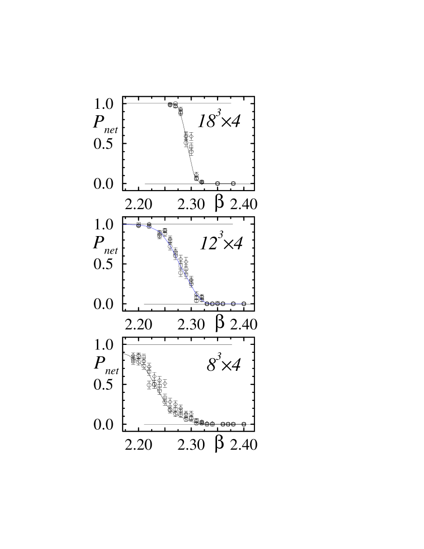
Figure 1:

Figure 2:

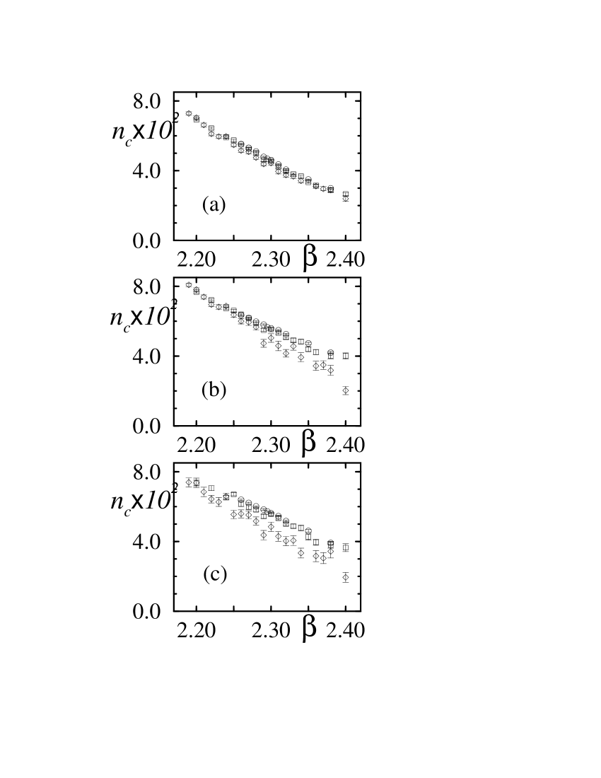
Figure 3:

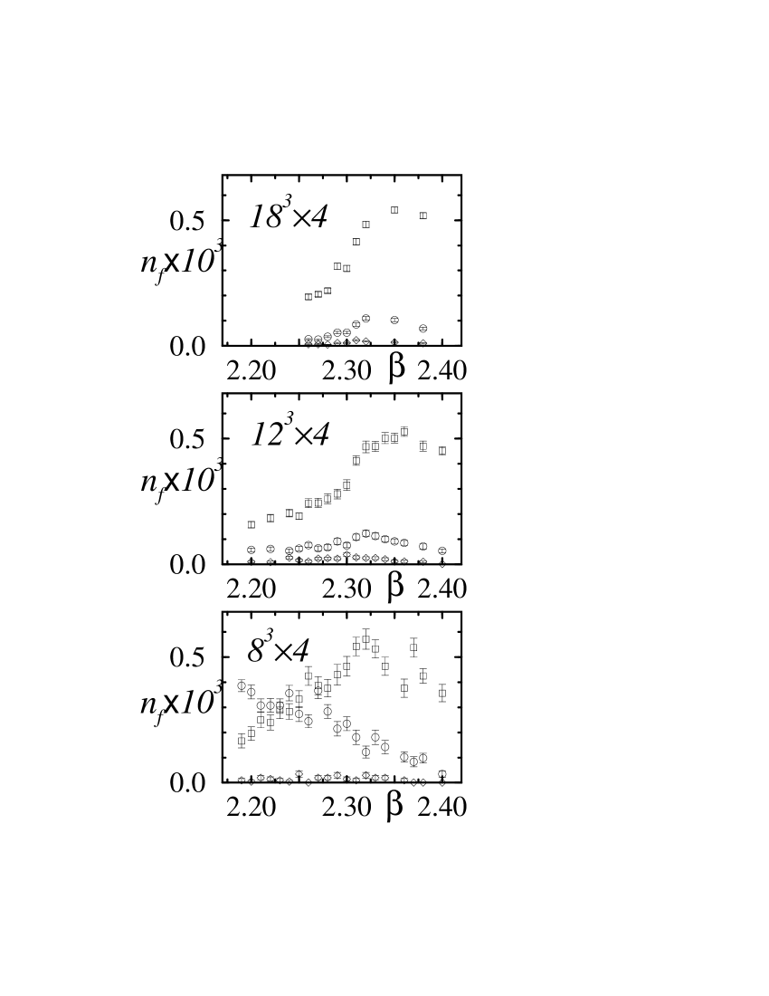
Figure 4:

References

- [1] G. ’t Hooft, in: High Energie Physics, ed A. Zichichi (Editorice Compositori, Bologna 1976).
- [2] S. Mandelstam Phys. Rep. 23 C (1976) 245.
- [3] T. Banks, R. Myerson and J. Kogut, Nucl. Phys. B 129 (1977) 493.
- [4] T.A. DeGrand and D. Toussaint, Phys. Rev. D 22 (1980) 2478.
- [5] G. ’t Hooft, Nucl. Phys. B 190 (1981) 455.
- [6] A.S. Kronfeld, G.Schierholz and U.-J. Wiese, Nucl. Phys. B 293 (1987) 461.
- [7] A.S. Kronfeld, M.L. Laursen, G.Schierholz and U.-J. Wiese, Phys. Lett. B 198 (1987) 516.
- [8] M.I. Polikarpov, preprint KANAZAWA-96-19; hep-lat/9609020.
- [9] F. Brandstaeter, G. Schierholz and U.-J. Wiese, Phys. Lett. B 272 (1991) 319.
- [10] V.G. Bornyakov, V.K. Mitrjushkin and M. Müller-Preussker, Phys. Lett. B 284 (1992) 99.
- [11] T.L. Ivanenko, A.V. Pochinsky and M.I. Polikarpov, Phys. Lett. B 302 (1993) 458.
- [12] S. Ejiri, S. Kitahara, Y. Matsubara and T. Suzuki, Phys. Lett. B 343 (1995) 304.
- [13] S. Kitahara, Y. Matsubara and T. Suzuki, Prog. Theor. Phys. 93 (1995) 1.
- [14] S. Ejiri, Phys. Lett. B 376 (1996) 163.
- [15] W. Kerler, C. Rebbi and A. Weber, Phys. Rev. D 50 (1994) 6984.
- [16] W. Kerler, C. Rebbi and A. Weber, Phys. Lett. B 348 (1995) 565.
- [17] W. Kerler, C. Rebbi and A. Weber, Phys. Lett. B 380 (1996) 346.
- [18] J.W. Essam, p. 197 in Phase Transitions and Critical Phenomena, Vol. 2, eds. C. Domb and M.S. Green (Academic Press, London, 1972).
- [19] M. Aizenman, J. Bricmont and J.L. Lebowitz, J. Stat. Phys. 49 (1987) 859.
- [20] M. Baig, H. Fort and J.B. Kogut, Phys. Rev. D 50 (1994) 5920.
- [21] A. Bode, T. Lippert and K. Schilling, Nucl. Phys. B (Proc. Suppl.) 34 (1994) 549.
- [22] J.E. Mandula and M. Ogilvie, Phys. Lett. B 248 (1990) 156.
- [23] S. Hioki, S. Kitahara, Y. Matsubara, O. Miyamura, S. Ohno and T. Suzuki, Phys. Lett. B 271 (1991) 201.
- [24] S. Hioki, S. Kitahara, Y. Matsubara, O. Miyamura, S. Ohno and T. Suzuki, Phys. Lett. B 285 (1992) 343.
- [25] Ph. de Focrand and R. Gupta, Nucl. Phys. B (Proc. Suppl.) 9 (1989) 516.
- [26] S. Kirkpatrick, C.D. Gerlatt Jr. and M.P. Vecchi, Science 220 (1983) 671.
- [27] G.S. Bali, V. Bornyakov, M. Müller-Preussker and F. Pahl, Nucl. Phys. B (Proc. Suppl.) 42 (1995) 852.
- [28] J. Engels, S. Mashkevich, T. Scheideler and G. Zinovjev, Phys. Lett. B 365 (1996) 219.
- [29] J. Smit and A.J. van der Sijs, Nucl. Phys. B 355 (1991) 603.