hep-lat/9701016

SWAT/97/136

January 1997

The Three Dimensional Thirring Model for Small $N_{f}$

L. Del Debbio, S.J. Hands, J.C. Mehegan

(the UKQCD collaboration)

Department of Physics, University of Wales Swansea,

Singleton Park, Swansea SA2 8PP, U.K.

Abstract

We formulate the three dimensional Thirring model on a spacetime lattice and study it for various even numbers of fermion flavors $N_{f}$ by Monte Carlo simulation. We find clear evidence for spontaneous chiral symmetry breaking at strong coupling, contradicting the predictions of the $1/N_{f}$ expansion. The critical point appears to correspond to an ultra-violet fixed point of the renormalisation group; a fit to a RG-inspired equation of state in the vicinity of the fixed point yields distinct critical exponents for $N_{f}=2$ and $N_{f}=4$, while no fit is found for $N_{f}=6$, suggesting there is a critical number $N_{fc}<6$ beyond which no chiral symmetry breaking occurs. The spectrum of the $N_{f}=2$ theory is studied; the states examined vary sharply but continuously across the transition.

PACS: 11.10.Kk, 11.30.Rd, 11.15.Ha

Keywords: four-fermi, Monte Carlo simulation, dynamical fermions, chiral symmetry breaking, renormalisation group fixed point

1 Introduction

The Thirring model is a quantum field theory of fermions interacting via a current-current contact term, described in three dimensional continuum Euclidean spacetime by the following Lagrangian:

$${\cal L}=\bar{\psi}_{i}(\partial{\!\!\!/}\,+m)\psi_{i}+{g^{2}\over{2N_{f}}}(\bar{\psi}_{i}\gamma_{\mu}\psi_{i})^{2}.$$ (1.1)

Here $\psi$ and $\bar{\psi}$ are four-component spinors, $m$ is a bare mass, and $i$ runs over $N_{f}$ fermion species. After the introduction of an auxiliary vector field, the above Lagrangian can be rewritten as:

$${\cal L}_{aux}=\bar{\psi}_{i}(\partial{\!\!\!/}\,+iA{\!\!\!/}\,+m)\psi_{i}+{N_{f}\over{2g^{2}}}(A_{\mu})^{2}$$ (1.2)

which now contains the fermionic bilinear term of the usual QED lagrangian but with a mass term for the vector field, which spoils the gauge-invariance of ${\cal L}_{aux}$. This is no surprise, since the original lagrangian did not show any local symmetry. The global symmetries are a $U(N_{f})$ one, corresponding to rotations in flavor space, and, for $m\rightarrow 0$, a $U(N_{f})_{A}$ chiral symmetry. Since the coupling constant $g$ has mass dimension $[g]=(1-{d\over 2})=-{1\over 2}$, the usual perturbative expansion is non-renormalisable. However perturbation theory is not the end of the story and, as suggested several years ago [1, 2], different approaches can yield a well-defined continuum limit, corresponding to a UV–stable fixed point of the renormalisation group (RG).

The Gross–Neveu model (GN), which has been studied both numerically and in the $1/N_{f}$ expansion [3, 4, 5], exhibits this behaviour. The model turns out to be renormalisable to all orders in $1/N_{f}$, with a UV–stable RG fixed point at $g_{UV}\neq 0$ and chiral symmetry breaking for $g>g_{UV}$; only for $g\simeq g_{UV}$ can the ratio of the physical scale (either a particle mass or a scattering cross-section) to the UV cutoff be made small. The theory defined at this point describes the IR dynamics of a linear sigma model with a Yukawa coupling to fermions [6], which is super-renormalisable about the origin:

$${\cal L}_{Yu}=\bar{\psi}(\partial{\!\!\!/}\,+v\sigma+m)\psi+\frac{1}{2}(\partial\sigma)^{2}+\frac{1}{2}\mu^{2}\sigma^{2}+\lambda\sigma^{4}$$ (1.3)

For a critical value of $v$ in the IR regime the kinetic and quartic terms of the $\sigma$-field become irrelevant operators and thus the system equivalent to the GN model. The critical behaviour for the GN model can be summarised by the behaviour of the $\beta$-function, as shown in Fig. 1. In two dimensions, the theory is asymptotically free, and the $\beta$-function exhibits the usual UV fixed point at the origin. For $2<d<4$, the fixed point is shifted away from the origin, separating a strong coupling regime, where dynamical chiral symmetry breaking is possible, from a weak coupling phase where the theory is chirally symmetric [7].

The situation for the Thirring model is less clear. At both leading and next-to-leading order in $1/N_{f}$ the renormalisability of the massless model has been established [8]. For $d<4$ the vacuum polarisation is actually UV–finite so long as the regularisation respects current conservation. As a consequence a continuum limit may be defined for any value of the coupling $g$, which would control, e.g., the ratio of physical fermion mass to vector bound state mass. In other words, the $\beta$-function is vanishing for any value of $g$ and the interaction $(\bar{\psi}_{i}\gamma_{\mu}\psi_{i})^{2}$ is a marginal operator, whereas the interaction for the GN model is relevant [9]. Another prediction of the $1/N_{f}$ expansion is the vanishing of the vector bound state mass in the strong coupling limit $mg\rightarrow\infty$. A massless particle mediating an interaction between conserved currents suggests an equivalence between the UV behaviour of Thirring model and the IR one of $\mbox{QED}_{3}$, which would thus be the analogue of the equivalence between the GN and Yukawa models. Such a conjecture is supported by the fact that the $O(1/N_{f})$ corrections in the two models appear to coincide [8, 10]. Moreover in the $1/N_{f}$ expansion, as in perturbative gauge theory, no diagram ever appears resulting in the dynamical breaking of chiral symmetry leading to spontaneous mass generation.

The prediction of no spontaneous mass generation is contradicted, however, by results from a completely non-perturbative approach, namely solution of Schwinger–Dyson (SD) equations, which predicts a non-vanishing chiral condensate $\langle\bar{\psi}\psi\rangle$ in the limit $m\rightarrow 0$ [2, 11, 12]. In this approach a non-trivial solution for the dressed fermion propagator $S(p)=(A(p)ip{\!\!\!/}\,+\Sigma(p))^{-1}$ is sought, i.e. one in which the self-energy $\Sigma(p)$ and hence $\langle\bar{\psi}\psi\rangle$ are non-vanishing in the chiral limit $m\to 0$. Unfortunately, the SD equations can only be solved by truncating them in a somewhat arbitrary fashion. The usual approximation [2, 12], is to assume that the vector propagator is given by its leading-order form for $m=0$ in the $1/N_{f}$ expansion, viz.

$$D_{\mu\nu}(k)=\left(\delta_{\mu\nu}-{{k_{\mu}k_{\nu}}\over k^{2}}\right)\left(1+{{g^{2}(k^{2})^{1\over 2}}\over 8}\right)^{-1}+{{k_{\mu}k_{\nu}}\over k^{2}}$$ (1.4)

and that the fermion-vector vertex function is well-approximated by the bare vertex (the so-called “planar” or “ladder” approximation):

$$\Gamma_{\mu}(p,q)=-{{ig}\over\sqrt{N_{f}}}\gamma_{\mu}.$$ (1.5)

The most systematic treatment has been given by Itoh et al [12], who note the equivalence of (1.2) to a gauge-fixed form of a gauged fermion-scalar model. This allows the specification of an alternative non-local gauge-fixing condition, which in turn entails $A(p)\equiv 1$, with no effect, of course, on gauge-invariant quantities such as the physical mass or $\langle\bar{\psi}\psi\rangle$. The resulting SD equations can be solved exactly in the limit $g^{2}\to\infty$; a non-trivial solution for $\Sigma(p)$ exists for

$$N_{f}<N_{fc}={128\over{3\pi^{2}}}\simeq 4.32.$$ (1.6)

This is identical to the critical $N_{fc}$ predicted for non-trivial IR behaviour in $\mbox{QED}_{3}$ [13]. However, since the integral equations require the introduction of a UV cutoff $\Lambda$, a feature of this solution is that the induced physical scale $\mu$ depends on $N_{f}$ in an essentially singular way:

$${\mu\over\Lambda}\propto\exp\left(-{2\pi\over\sqrt{{N_{fc}\over N_{f}}-1}}\right);\;\;\;\langle\bar{\psi}\psi\rangle\propto\Lambda^{1\over 2}\mu^{3\over 2}\propto\exp\left(-{3\pi\over\sqrt{{N_{fc}\over N_{f}}-1}}\right)$$ (1.7)

This implies that in the strong coupling limit a continuum limit only exists as $N_{f}\to N_{fc}$.

The behaviour (1.7) is an example of an infinite order, or “conformal” phase transition, originally discussed in a particle physics context by Miranskii and collaborators in quenched $\mbox{QED}_{4}$ [14], and recently discussed in more generality [15]. One prediction of [15] is that although the order parameter $\langle\bar{\psi}\psi\rangle$ is continuous at the transition, there is a discontinuity in the spectrum of light excitations, with no light scalar resonances on the symmetric side of the transition. In the broken phase, of course, Goldstone’s theorem predicts light pions. This behaviour has recently been exhibited in an investigation of four dimensional SU($N_{c}$) gauge theory with an intermediate number $N_{f}$ of fermion flavors [16]: a solution of the Bethe-Salpeter equation in ladder approximation found no low-momentum pole in the symmetric phase.

Unfortunately no analytic solution to the SD equation for the Thirring model exists for $g^{2}<\infty$; however using different techniques Kondo [17] has argued that there is a critical line $N_{fc}(g^{2})$ in the $(g^{2},N_{f})$ plane, which is a smooth invertible function. Therefore for integer $N_{f}<N_{fc}$ one might conjecture the form [18]

$$\langle\bar{\psi}\psi\rangle\propto\exp\left(-{a\over\sqrt{{g^{2}\over g_{c}^{2}}-1}}\right),$$ (1.8)

corresponding to a symmetry restoring transition at some critical point $g^{2}=g_{c}^{2}(N_{f})$. Presumably in this scenario the coupling $g$ has become relevant: there may exist a novel strongly-coupled continuum limit at the critical point not described by the $1/N_{f}$ expansion, which is simultaneously the UV limit of the Thirring model and the IR limit of $\mbox{QED}_{3}$. Since there is no small dimensionless parameter in play, this fixed point would be inherently non-perturbative. It is worth mentioning in passing that a novel IR fixed point in $\mbox{QED}_{3}$ has been proposed by Aitchison and Mavromatos in connection with non-Fermi liquid behaviour in the normal phase of superconducting cuprates [19].

Although this scenario of a non-trivial fixed point for $N_{f}<N_{fc}$ is attractive, there are good reasons to be cautious. Using a different sequence of truncations Hong and Park have found chiral symmetry breaking for all $N_{f}$ [11], with

$${1\over g_{c}^{2}}\propto\exp\left(-{{N_{f}\pi^{2}}\over 16}\right),$$ (1.9)

a result which is also non-analytic in $1/N_{f}$ and hence beyond the reach of the $1/N_{f}$ perturbative series. Moreover in $\mbox{QED}_{3}$, studies beyond the planar approximation, using improved ansätze for the vertex $\Gamma_{\mu}$, suggest that the condition $A(p)\equiv 1$ is unphysical, and that chiral symmetry is spontaneously broken for all $N_{f}$  [20]. In the current context this would imply $g_{c}^{2}<\infty$ for all $N_{f}$.

Because of the systematic uncertainty attached to the SD approach, and because of the intrinsic interest in exploring the non-perturbative behaviour of a fermionic model, we have studied the three dimensional Thirring model by Monte Carlo simulation on a spacetime lattice. Our initial results appeared in [18], where we claimed that critical points with distinct critical indices exist for the models with $N_{f}=2,4$, but that evidence for a critical theory with $N_{f}=6$ was not found. In this paper we summarise those results, and present further data which enable us to refine our description of the critical behaviour of the $N_{f}=2$ model. In Sec. 2 we give a fairly lengthy exposition of the lattice formulation, showing that the lattice method is itself not without systematic uncertainties. Although we use staggered lattice fermions which have a continuous remnant of the $\mbox{U}(N_{f})_{A}$ axial symmetry, a transcription to a basis in which the Fermi fields have explicit spin and flavor indices reveals that there are many other interactions present at tree level besides the desired current-current form. Perhaps a robust counter-argument to this problem is that for a strongly-coupled fixed point a non-perturbative regularisation is always necessary, and therefore “what you see is what you get”, i.e. the fixed point theory defines itself via its critical exponents and spectral quantities. In addition, the lattice form of the current is not exactly conserved, resulting in an additive renormalisation of the inverse coupling $1/g^{2}$. This makes it difficult in practice to identify the strong coupling limit $g^{2}\to\infty$. A description of the simulation, and a list of the measured observables, namely the condensate, susceptibilities and propagators, follows.

In Sec. 3 we present results for the equation of state, i.e. $m=f(\langle\bar{\psi}\psi\rangle,g)$. Since it is impossible to work directly in the chiral limit $m=0$, we find it convenient to fit to a phenomenological form inspired by the standard power-law scaling form used in the theory of ferromagnetism, with its attendant critical exponents $\beta,\gamma,\delta$ and $\nu$, together with the additional constraints of hyperscaling, and, from the ladder approach to the gauged Nambu – Jona-Lasinio model [21], that $\delta-1/\beta=\gamma\equiv 1$. We justify this approach not so much by any theoretical argument but because its shortcomings if any should manifest themselves as variations in the fitted values of the exponents as data is taken from systems on larger volumes and closer to the chiral limit. In [18] the fitted exponents for the $N_{f}=2,4$ models were distinct, a feature not seen in similar studies of $\mbox{QED}_{4}$ [22, 23]. Here we supplement the data of [18] for $N_{f}=2$ with results from a larger lattice $(16^{3})$ and a smaller bare mass $m$, and refine the fit by combining data from several lattice volumes in a finite size scaling analysis. We find critical exponents and $g_{c}^{2}$ completely consistent with those of our earlier studies, which strengthens the case for a critical point described by power-law scaling. We also have some new results for the $N_{f}=6$ model on $12^{3}$ systems, supporting our previous claim that there is no transition in this case, and hence that $N_{fc}<6$ for the Thirring model.

In Sec. 4 we present exploratory results for susceptibilities, and for fermion and bound-state masses. Our lattice size of $16^{3}$ is unfortunately not long enough in the temporal direction to permit real accuracy; nonetheless qualitative features of the level ordering in either phase do emerge. The susceptibilities reflect the phase transition very nicely, with longitudinal and transverse susceptibilities $\chi_{l}$ and $\chi_{t}$ varying from near-degeneracy in the symmetric phase (thus indirectly supporting the hypothesis $\delta-1/\beta=1$) to $\chi_{t}\gg\chi_{l}$ in the broken phase. The effects of dynamical fermion loops in the quantum vacuum can also be estimated, and appear to become dominant in the broken phase. The fermion, pseudoscalar and scalar masses all behave as expected, the pion mass staying small and roughly constant, while fermion and scalar masses change sharply but continuously across the transition. There is no sign of the discontinuities described in [15]. Finally studies in the vector-like channel reveal light states both with vector and axial vector quantum numbers in the symmetric phase. This is interesting because no light axial vector is predicted in the continuum $1/N_{f}$ expansion at leading order, as we show in Sec. 4. Both states become difficult to observe in the broken phase. Our conclusions are presented in Sec. 5.

2 Lattice formulation

We want to discretise the action of Eq. (1.1) on a hypercubic Euclidean lattice. In order to recover a partial $U(N)_{A}$ axial symmetry in the massless limit, we use $N$ flavors of staggered fermions. The lattice action then reads:

$$S = \frac{1}{2}\sum_{x\mu i}\bar{\chi}_{i}(x)\eta_{\mu}(x)\left[\chi_{i}(x+\hat{\mu})-\chi_{i}(x-\hat{\mu})\right]+$$ (2.1)

$$m\sum_{xi}\bar{\chi}_{i}(x)\chi_{i}(x)+\frac{g^{2}}{2N}\sum_{x\mu ij}\bar{\chi}_{i}(x)\chi_{i}(x+\hat{\mu})\bar{\chi}_{j}(x+\hat{\mu})\chi_{j}(x)$$

where $\chi,\bar{\chi}$ are the staggered fermion fields, $\eta_{\mu}$ the Kawamoto–Smit phases, $m$ is the bare fermion mass, the flavor indices $i,j$ run from $1$ to $N$ and the vector character of the interaction is encoded in the geometrical structure of the four fermion term.

To express the action as a bilinear in $\chi,\bar{\chi}$, which makes it amenable to simulation, we introduce a bosonic auxiliary field as in (1.2). In this paper we choose a form which we will refer to as non-compact:

$$S = \frac{1}{2}\sum_{x\mu i}\bar{\chi}_{i}(x)\eta_{\mu}(x)(1+iA_{\mu}(x))\chi_{i}(x+\hat{\mu})+\mbox{h.c.}$$ (2.2)

$$+m\sum_{xi}\bar{\chi}_{i}(x)\chi_{i}(x)+\frac{N}{4g^{2}}\sum_{x\mu}A_{\mu}(x)^{2}$$

$$\equiv \sum_{xyi}\bar{\chi}_{i}(x)M[A,m](x,y)\chi_{i}(y)+\frac{N}{4g^{2}}\sum_{x\mu}A_{\mu}(x)^{2}$$

where we have introduced $M[A,m]$ to denote the fermionic bilinear, which depends on both the auxiliary field and the bare mass. It is straightforward to integrate over the auxiliary field and recover Eq. (2.1).

In the chiral limit $m\to 0$ both the original action (2.1) and the bosonised form (2.2) are invariant under a global axial rotation, which for $N=1$ is written

$$\chi(x)\mapsto\exp(i\alpha\varepsilon(x))\chi(x)\;\;\;;\;\;\;\bar{\chi}(x)\mapsto\exp(i\alpha\varepsilon(x))\bar{\chi}(x),$$ (2.3)

where the phase $\varepsilon(x)=(-1)^{x_{1}+x_{2}+x_{3}}$. The generalisation to U(N) is straightforward. We will refer to this as the chiral symmetry of the model. In the $m\to 0$ limit for certain values of the coupling $g^{2}>g_{c}^{2}(N)$ it is spontaneously broken, signalled by the appearance of a condensate $\langle\bar{\chi}\chi\rangle\not=0$.

Some comments on the lattice formulation are appropriate. Eq. (2.2) in the long wavelength limit (i.e. assuming $a\partial\psi\ll\psi$) is clearly closely related to the continuum auxiliary form (1.2), and as such is suitable for a perturbative expansion in small-mode fluctuations of the $A_{\mu}$ fields, corresponding to the continuum $1/N_{f}$ expansion. This expansion is well-behaved because to leading order the vector propagator $D_{\mu\nu}(x)=\langle A_{\mu}(0)A_{\nu}(x)\rangle$ receives a contribution not just from the quadratic term $A_{\mu}^{2}$, but also from the vacuum polarisation loop $\Pi_{\mu\nu}$, which is finite in $d<4$. We find in the deep Euclidean region [8] (Cf. (1.4))

$$\lim_{k^{2}\to\infty}D_{\mu\nu}(k)\propto{\cal P}_{\mu\nu}(k){1\over\sqrt{k^{2}}}+\mbox{longitudinal}$$ (2.4)

where ${\cal P}_{\mu\nu}$ is the transverse projector

$${\cal P}_{\mu\nu}(k)=\delta_{\mu\nu}-{{k_{\mu}k_{\nu}}\over k^{2}}.$$ (2.5)

Because the interaction current $\bar{\psi}\gamma_{\mu}\psi$ is conserved, the longitudinal component of $D_{\mu\nu}$ has no physical significance [1][12][17]. The $1/k$ behaviour of $D_{\mu\nu}$ in effect suppresses short wavelength excitations of the auxiliary field, and justifies the long-wavelength expansion a posteriori. It means we might hope the form (2.2) has the correct continuum limit. This assumption may not be justified, however, due to the chiral phase transition at finite $g^{2}$. Since the $1/N_{f}$ expansion predicts no phase transition, we know that there will be at least some part of coupling constant space where the above arguments cannot hold. In this case it is not quite so clear that (2.2) coincides with the continuum form (1.1).

To see why there might be a problem, we must consider the continuum flavor interpretation of the lattice action (2.1). First define a unitary transformation to fields $q,\bar{q}$ [24]:

$$q^{\alpha a}_{i}(y)=\left(\matrix{u^{\alpha a}_{i}(y)\cr d^{\alpha a}_{i}(y)\cr}\right)={1\over{4\surd{2}}}\sum_{P}\left(\matrix{\Gamma^{\alpha a}_{P}&\cr&B^{\alpha a}_{P}\cr}\right)\chi_{i}(P;y),$$ (2.6)

where $y$ denotes a site on a lattice of spacing $2a$ and $P$ is a 3-vector with entries either 0 or 1 ranging over corners of the elementary cube associated with $y$, so that each side of the original lattice corresponds to a unique choice of $(P;y)$. The $2\times 2$ matrices $\Gamma_{P}$ and $B_{P}$ are defined by

$$\Gamma_{P}=\tau_{1}^{P_{1}}\tau_{2}^{P_{2}}\tau_{3}^{P_{3}}\;\;\;;\;\;\;B_{P}=(-\tau_{1})^{P_{1}}(-\tau_{2})^{P_{2}}(-\tau_{3})^{P_{3}},$$ (2.7)

where $\tau_{\mu}$ are the Pauli matrices. It is then possible to recast the bilinear term of (2.1) as follows;

$$S_{kin} = (2a)^{3}\sum_{y\mu}\biggl{(}\bar{q}_{i}(y)(\gamma_{\mu}\otimes 1\kern-4.5pt1_{2}){[q_{i}(y+\hat{\mu})-q_{i}(y-\hat{\mu})]\over{4a}}+$$ (2.8)

$$\bar{q}_{i}(y)(\gamma_{4}\otimes\tau_{\mu}^{*}){[q_{i}(y+\hat{\mu})+q_{i}(y-\hat{\mu})-2q_{i}(y)]\over{4a}}\biggr{)}+$$

$$m(2a)^{3}\sum_{y}\bar{q}_{i}(y)(1\kern-4.5pt1_{4}\otimes 1\kern-4.5pt1_{2})q_{i}(y).$$

The direct product is between $4\times 4$ Dirac matrices, acting on spinor degrees of freedom, defined by

$$\gamma_{\mu}=\left(\matrix{\tau_{\mu}&\cr&-\tau_{\mu}\cr}\right)\;\;\;;\;\;\;\gamma_{4}=\left(\matrix{&-i1\kern-4.5pt1_{2}\cr i1\kern-4.5pt1_{2}&\cr}\right)\;\;\;;\;\;\;\gamma_{5}=\left(\matrix{&1\kern-4.5pt1_{2}\cr 1\kern-4.5pt1_{2}&\cr}\right),$$ (2.9)

and $2\times 2$ matrices acting on flavor degrees of freedom. Each lattice fermion flavor in three dimensions corresponds to two continuum four-component spinor flavors. Hence

$$N_{f}=2N.$$ (2.10)

In terms of this new basis the chiral symmetry of the model (2.3) reads

$$q\mapsto\exp(i\alpha(\gamma_{5}\otimes 1\kern-4.5pt1))q\;\;\;;\;\;\;\bar{q}\mapsto\bar{q}\exp(i\alpha(\gamma_{5}\otimes 1\kern-4.5pt1)).$$ (2.11)

The condensate $\langle\bar{\chi}\chi\rangle$ in the new basis reads $\langle\bar{q}(1\kern-4.5pt1\otimes 1\kern-4.5pt1)q\rangle$.

The first and third terms of (2.8) are clearly of the same form as the continuum action for free massive fermions, whereas the second term, which is flavor non-singlet and Lorentz non-covariant, is formally $O(a)$ and hence hopefully irrelevant. The problem comes when we consider the interaction term. In the auxiliary field formalism, only in the long-wavelength limit would we expect the interaction to assume its expected continuum form $A_{\mu}\bar{q}_{i}(\gamma_{\mu}\otimes 1\kern-4.5pt1_{2})q_{i}$ [25]. When $A$ is integrated out to recover the original form (2.1) though, all momentum modes are summed over with equal weight. In fact, in four-fermi form the interaction contains many extra terms:

$$S_{int} = {g^{2}\over{2N}}\times{(2a)^{3}\over 2}\times\sum_{y\mu ij}$$ (2.12)

$$\biggl{[}\Bigl{(}\bar{q}_{i}(y)(\gamma_{\mu}\otimes 1\kern-4.5pt1)(1+f_{\mu})q_{i}(y)+\bar{q}_{i}(y)(i\gamma_{4}\otimes\tau_{\mu}^{*})\delta_{\mu}q_{i}(y)\Bigr{)}\times$$

$$\Bigl{(}(1+f_{\mu})\bar{q}_{j}(y)(\gamma_{\mu}\otimes 1\kern-4.5pt1)q_{j}(y)+\delta_{\mu}\bar{q}_{j}(y)(-i\gamma_{4}\otimes\tau_{\mu}^{*})q_{j}(y)\Bigr{)}$$

$$+ \Bigl{(}\bar{q}_{i}(y)(\gamma_{5}\gamma_{\mu}\otimes 1\kern-4.5pt1)(1+f_{\mu})q_{i}(y)+\bar{q}_{i}(y)(i\gamma_{5}\gamma_{4}\otimes\tau_{\mu}^{*})\delta_{\mu}q_{i}(y)\Bigr{)}\times$$

$$\Bigl{(}(1+f_{\mu})\bar{q}_{j}(y)(\gamma_{\mu}\gamma_{5}\otimes 1\kern-4.5pt1)q_{j}(y)+\delta_{\mu}\bar{q}_{j}(y)(-i\gamma_{4}\gamma_{5}\otimes\tau_{\mu}^{*})q_{j}(y)\Bigr{)}$$

$$+ \sum_{\nu}\Bigl{(}\bar{q}_{i}(y)(i\gamma_{4}\gamma_{5}\gamma_{\nu}\gamma_{\mu}\otimes\tau_{\nu}^{*})(1+f_{\mu})q_{i}(y)+\bar{q}_{i}(y)(\gamma_{\nu}\gamma_{5}\otimes\tau_{\nu}^{*}\tau_{\mu}^{*})\delta_{\mu}q_{i}(y)\Bigr{)}\times$$

$$\Bigl{(}(1+f_{\mu})\bar{q}_{j}(y)(i\gamma_{4}\gamma_{5}\gamma_{\mu}\gamma_{\nu}\otimes\tau_{\nu}^{*})q_{j}(y)+\delta_{\mu}\bar{q}_{j}(y)(-\gamma_{\nu}\gamma_{5}\otimes\tau_{\mu}^{*}\tau_{\nu}^{*})q_{j}(y)\Bigr{)}$$

$$+ \sum_{\nu}\Bigl{(}\bar{q}_{i}(y)(-i\gamma_{4}\gamma_{\nu}\gamma_{\mu}\otimes\tau_{\nu}^{*})(1+f_{\mu})q_{i}(y)+\bar{q}_{i}(y)(-\gamma_{\nu}\otimes\tau_{\nu}^{*}\tau_{\mu}^{*})\delta_{\mu}q_{i}(y)\Bigr{)}\times$$

$$\Bigl{(}(1+f_{\mu})\bar{q}_{j}(y)(i\gamma_{4}\gamma_{\mu}\gamma_{\nu}\otimes\tau_{\nu}^{*})q_{j}(y)+\delta_{\mu}\bar{q}_{j}(y)(-\gamma_{\nu}\otimes\tau_{\mu}^{*}\tau_{\nu}^{*})q_{j}(y)\Bigr{)}\biggr{]},$$

where the difference operators $f$ and $\delta$ are defined by

$$f_{\mu}q(y)={1\over 2}\left(q(y+\hat{\mu})+q(y-\hat{\mu})\right)\;\;\;;\;\;\;\delta_{\mu}q(y)={1\over 2}\left(q(y+\hat{\mu})-q(y-\hat{\mu})\right).$$ (2.13)

The terms containing $\delta$ are formally $O(a)$ and hence probably irrelevant, but no such argument can be used for the remainder, which, in addition to the desired form $(\bar{q}_{i}(\gamma_{\mu}\otimes 1\kern-4.5pt1)q_{i})^{2}$, contains extra flavor non-singlet and non-covariant terms. If the $1/N_{f}$ expansion were valid, then one could argue that only interactions between conserved currents would generate long-range correlations between the $A$ fields, and that all other interactions would become irrelevant in the continuum limit – a similar effect appears to be the case in other two [27, 28] and three [3] dimensional four-fermi models where a renormalisable expansion is available. Even in this case there might also be contributions in the chiral limit from the interaction $(\bar{q}_{i}(\gamma_{\mu}\gamma_{5}\otimes 1\kern-4.5pt1)q_{i})^{2}$. However, as argued above, in the present case we know the $1/N_{f}$ expansion fails qualitatively in the chirally broken phase. It therefore becomes a matter of experiment, by studying the current-current and $AA$ correlations in various channels numerically, to determine the continuum limit of the action (2.1).

A second issue we must address is that despite the above comments there is an important difference between the continuum $1/N_{f}$ expansion and the $1/N$ expansion applied to the non-compact lattice action (2.2). This concerns vector current conservation. In the continuum model a regularisation such as Pauli-Villars, which conserves the interaction current, must be assumed in order to ensure that the superficial $O(\Lambda)$ contribution to vacuum polarisation vanishes, leaving a finite result [1, 2, 8]. Now, in non-compact lattice $\mbox{QED}_{3}$, the vacuum polarisation is again UV finite, but this time because of a cancellation between $O(a^{-1})$ contributions from two separate diagrams (Fig. 2 - see eg. [29]). The second diagram appears because the gauge-invariant interaction term in QED is $\bar{\chi}\exp(ieA_{\mu})\chi$, and hence contains $n$-photon-electron-positron vertices. In the action (2.2), on the other hand, the interaction is $\bar{\chi}iA_{\mu}\chi$, so only the left-hand diagram is present. Therefore cancellation of $O(a^{-1})$ divergences does not occur. We find for the vacuum polarisation tensor to leading order in $1/N$:

$$\displaystyle\lim_{k^{2}a^{2}\to 0}\Pi_{\mu\nu}^{LATT}(k)={\cal P}_{\mu\nu}(k)\Pi^{CONT}(k^{2},m)+{g^{2}\over a}\delta_{\mu\nu}J(m),$$ (2.14)

where

$$J(m)=2\int_{-\pi}^{\pi}{{d^{3}q}\over(2\pi)^{3}}{{\sin^{2}q_{\mu}}\over{\sum_{\nu}\sin^{2}q_{\nu}+m^{2}}}\;\;\;;\;\;\;\displaystyle\lim_{m\to 0}J(m)={2\over 3},$$ (2.15)

and, recalling a factor of two from (2.10)

$$\Pi^{CONT}(k^{2},m)=-{g^{2}\over\pi}\left[m+{(k^{2}-4m^{2})\over{2\sqrt{k^{2}}}}\tan^{-1}\left({\sqrt{k^{2}}\over{2m}}\right)\right].$$ (2.16)

This means that for the inverse auxiliary propagator (setting $a=1$)

$$D_{\mu\nu}^{-1}(k) = \delta_{\mu\nu}-\Pi^{LATT}_{\mu\nu}(k)$$ (2.17)

$$= \delta_{\mu\nu}(1-g^{2}J(m))-{\cal P}_{\mu\nu}(k)\Pi^{CONT}(k^{2},m)$$

i.e.

$$D^{LATT}_{\mu\nu}(k)={1\over{1-g^{2}J(m)}}\left[{{{\cal P}_{\mu\nu}(k)}\over{1-{g^{2}\over{1-g^{2}J(m)}}\Pi^{CONT}(k^{2},m)}}+{{k_{\mu}k_{\nu}}\over{k^{2}}}\right].$$ (2.18)

If we compare this with the continuum result

$$D^{CONT}_{\mu\nu}(k)={{{\cal P}_{\mu\nu}(k)}\over{1-g^{2}\Pi^{CONT}(k^{2},m)}}+{{k_{\mu}k_{\nu}}\over k^{2}},$$ (2.19)

we see that the $O(a^{-1})$ divergence can be absorbed by a wavefunction renormalisation together with a coupling constant renormalisation:

$$A\mapsto A_{R}=(1-g^{2}J(m))^{1\over 2}A\;\;\;;\;\;\;g^{2}\mapsto g^{2}_{R}={g^{2}\over{1-g^{2}J(m)}}.$$ (2.20)

Now, the physics described by continuum $1/N_{f}$ perturbation theory occurs for the range of couplings $g^{2}_{R}\in[0,\infty)$, i.e. for $g^{2}\in[0,g^{2}_{lim})$, where to leading order

$$\displaystyle\lim_{m\to 0}{1\over g^{2}_{lim}}={2\over 3}.$$ (2.21)

We therefore expect discontinuous behaviour at bare coupling $g^{2}\simeq g^{2}_{lim}$, since at this point the auxiliary propagator is not defined (i.e. $D_{\mu\nu}^{-1}$ in (2.17) has no inverse). For $g^{2}>g^{2}_{lim}$, since $\Pi^{CONT}\to 0$ in the limit $k^{2}\to 0$, $D_{\mu\nu}$ becomes negative, suggesting that the model is not unitary in this region.

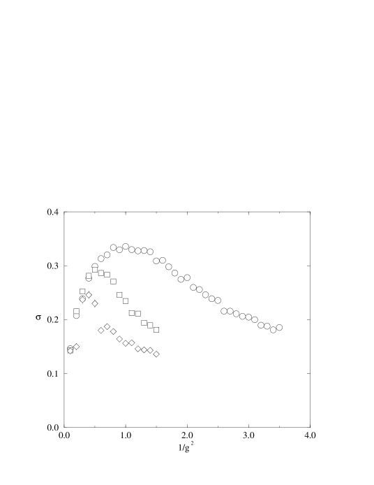
Figure 3: Chiral condensate $\sigma$ vs. $1/g^{2}$ for $N=1$ (circles), 2 (squares) and 3 (diamonds), showing discontinuous behaviour for $1/g^{2}\simeq 0.3$.

In Fig. 3 we plot $\sigma=\langle\bar{\chi}\chi\rangle$ vs. $1/g^{2}$ for $N=1,2,3$ and $m=0.10$ on a $8^{3}$ lattice [18]. The three models have apparently coincident condensates in the strong coupling region $1/g^{2}\leq 0.3$, which appear to be tending to zero in the $g^{2}\to\infty$ limit. It is tempting to associate this behaviour with $g^{2}>g^{2}_{lim}$, but the correspondence with the value (2.21) is not good. It may well be that the numerical value of the right-hand diagram of Fig. 2 is considerably reduced in a chirally broken vacuum; in any case we do not expect the $1/N$ expansion to be accurate here for the reasons described above.

The ill-defined behaviour of the $g^{2}\to\infty$ limit of the non-compact action (2.2) presents no problem for most of the simulation results presented in this paper, which focus on the critical region of the $N=1$ model around $1/g_{c}^{2}\simeq 2.0$, and of the $N=2$ model with $1/g_{c}^{2}\simeq 0.6$. However, we expect $g_{c}^{2}$ to increase as $N$ increases [11, 12, 17, 18], so that as models with larger $N$ are explored, eventually the relation between $g^{2}$ and $g_{R}^{2}$ will become important, particularly if lattice studies are to resolve the issue of the existence and value of $N_{fc}$. It is therefore worth making remarks on two other possible forms for the lattice Thirring model.

For $N=1$ there is an alternative but equivalent way of introducing the auxiliary field, which we will call the compact form:

$$S = \frac{1}{2}\sum_{x\mu i}\bar{\chi}_{i}(x)\eta_{\mu}(x)\left(1+\sqrt{{2g^{2}\over N}}\exp(i\theta_{\mu}(x))\right)\chi_{i}(x+\hat{\mu})+\mbox{h.c.}$$ (2.22)

$$+m\sum_{xi}\bar{\chi}_{i}(x)\chi_{i}(x),$$

where the link variables $\theta_{\mu}(x)$ are freely integrated over [30, 31]. It is straightforward to perform this integration to yield a term $\propto I_{0}(\sqrt{-2g^{2}\bar{\chi}(x)\chi(x+\hat{\mu})\bar{\chi}(x+\hat{\mu})\chi(x)})$, with $I_{0}$ a modified Bessel function. If we define $I_{0}$ by its power series expansion, then the Grassmann nature of the $\chi,\bar{\chi}$ truncates the expansion and forces equivalence with the partition function based on (2.1). We have performed some trial simulations using (2.22), and found identical results to those of the non-compact form (2.2) within statistical accuracy. It is interesting to note in passing that using a similar method one can show the equivalence of (2.1) with the strong gauge-coupling (i.e. $\beta=0$) limit of the gauge-fermion-scalar ($\chi U\phi$) model recently studied in connection with non-trivial continuum limits in 3 and 4 dimensions [32].

The bilinear action (2.22) can be extended to $N>1$ simply by introducing explicit flavor indices $i$ on $\chi,\bar{\chi}$. Now, however, terms of the form $(\bar{\chi}(x)\chi(x+\hat{\mu})\bar{\chi}(x+\hat{\mu})\chi(x))^{n}$ with $n>1$ are not suppressed by the Grassmann nature of $\chi$: for $N$ flavors of staggered fermion there are thus $n$-point couplings in the action with $n\leq 4N$. Since ultimately we wish to understand and contrast the behaviour of the Thirring model for various values of $N$, we prefer the non-compact form (2.2), where the interaction is of the same form for all $N$. It may well prove to be the case that in the RG sense the higher-point couplings are irrelevant, and hence (2.2) and (2.22) have identical continuum limits. Both variants deserve study.

Finally we mention a recent numerical study of a gauge-invariant version of the three dimensional Thirring model by Kim and Kim [33]; the action is

$$S = \frac{1}{2}\sum_{x\mu i}\bar{\chi}_{i}(x)\eta_{\mu}(x)\exp(i\theta_{\mu}(x))\chi_{i}(x+\hat{\mu})+\mbox{h.c.}$$ (2.23)

$$+m\sum_{xi}\bar{\chi}_{i}(x)\chi_{i}(x)-{N\over g^{2}}\sum_{x\mu}\cos(\phi(x+\hat{\mu})-\phi(x)+\theta_{\mu}(x)),$$

with $\phi$ a gauge-covariant scalar field. This action has a local gauge invariance by construction, corresponding to the hidden local symmetry noted in Refs. [12, 17]. In unitary gauge $\phi=1$ this action resembles (2.2) in the long-wavelength limit, but now has a periodic dependence on the auxiliary field. The main result of [33] is that the $N_{f}=6$ model appears qualitatively different from $N_{f}=2$, once again supporting a value of $N_{fc}<6$. It is an open question whether the action (2.23) lies in the same universality class as (2.1).

We simulated dynamical fermions using a hybrid Monte Carlo (HMC) algorithm. In all cases we used a random trajectory length drawn from a Poisson distribution with mean 0.9, and adjusted the timestep to maintain an acceptance rate of 70% or greater. Typically we performed measurements on configurations separated by between 2 and 5 trajectories. Our estimated autocorrelation times measured on sequences of configurations varied from $\sim 1$ to $\sim 3$ near the critical coupling; all our quoted errors take autocorrelations into account. The convergence criterion we used in the conjugate gradient matrix inversion was that the modulus of the residual vector was $10^{-6}$ per lattice site during guidance and $10^{-9}$ per site for Metropolis and measurement. Unlike the case of the GN model [3], we were unable to boost acceptance rates by tuning the parameters of the guidance Hamiltonian. However, the vectorlike nature of the interaction allows the simulation of the model for any value of the number of lattice species $N$, corresponding to a number of physical fermions $N_{f}=2N$, via an even-odd partitioning. For the very same reason, the only diagonal term in the fermion matrix comes from the mass term in the action. As $m$ gets small, we find that the fermion matrix becomes very difficult to invert. Simulations with small $m$ are therefore extremely time-consuming and represent a major problem for the extrapolation of the data to the chiral limit. Most of the results reported in this paper use between 200 and 500 measurements at each value of the coupling and bare mass. We have used periodic boundary conditions for the auxiliary field, and for the fermions used periodic in the spacelike directions and antiperiodic in the timelike direction. Most of the new results in the paper are obtained on $16^{3}$ lattices; however we also did some runs on an asymmetric $8^{2}\times 16$ lattice, to give some estimate of finite volume effects on correlation function measurements.

In our simulations we measured the following observables:

(i) The chiral condensate

$$\sigma=\langle\bar{\chi}\chi\rangle={1\over V}\langle\mbox{tr}M^{-1}\rangle,$$ (2.24)

where $M$ is the fermion kinetic operator introduced in eq.(2.2). In Sec. 3 we will discuss numerical fits to the model’s equation of state using these measurements. To enable alternative fitting procedures we list all our measurements made on symmetrical (i.e. $L^{3}$) lattices for $N_{f}=2$ in Tabs. 1 and 2, for $N_{f}=4$ in Tab. 3 and for $N_{f}=6$ in Tab. 4.

(ii) The longitudinal susceptibility

$$\chi_{l} = {1\over V}\sum_{x}\langle\bar{\chi}\chi(0)\;\bar{\chi}\chi(x)\rangle_{c}$$

$$= {1\over V}\sum_{x}\bigl{[}\langle(\mbox{tr}M^{-1})(\mbox{ tr}M^{-1})\rangle-\langle\mbox{tr}M^{-1}\rangle^{2}\bigr{]}-\langle\mbox{tr}(M^{-1}M^{-1})\rangle$$

$$\equiv \chi_{ls}+\chi_{lns},$$

where we have denoted the components with disconnected and connected fermion lines respectively as “singlet” $\chi_{ls}$ and “non-singlet” $\chi_{lns}$ in analogy with QCD flavor dynamics.

(iii) The transverse susceptibility

$$\chi_{t} = {1\over V}\sum_{x}\langle\bar{\chi}\varepsilon\chi(0)\;\bar{\chi}\varepsilon\chi(x)\rangle_{c}$$

$$= \chi_{ts}+\chi_{tns}$$

$$\equiv {1\over m}\langle\bar{\chi}\chi\rangle,$$

where we have used the fact that $\langle\bar{\chi}\varepsilon\chi\rangle$ vanishes, and the last line follows from a Ward identity.

(iv) The “vector susceptibility”

$$\chi_{v} = {1\over V}\sum_{x,\mu=1,2}\langle V_{\mu}(0)\;V_{\mu}(x)\rangle_{c}$$

$$= \chi_{vs}+\chi_{vns},$$

where $V_{\mu}$ is the interaction current:

$$V_{\mu}(x)={i\over 2}\bigl{(}\bar{\chi}(x)\eta_{\mu}(x)\chi(x+\hat{\mu})+\bar{\chi}(x+\hat{\mu})\eta_{\mu}(x)\chi(x)\bigr{)}.$$ (2.28)

Due to the inhomogeneous boundary conditions, we only averaged this quantity over the spacelike directions.

All susceptibilities, of course, are identical to the bound state propagator in the appropriate channel evaluated at zero momentum. The non-singlet components were therefore easily evaluated from the bound state correlators discussed below. The singlet parts, involving traces over a single power of $M^{-1}$, were evaluated using gaussian noise vectors. Since the susceptibility signals are intrinsically noisy, we used 5 noise vectors per configuration, thus obtaining 5 independent estimates of $\langle\bar{\chi}\chi\rangle$, and $5\times 4/2=10$ independent susceptibility estimates.

In addition to these operators we have also performed spectroscopy by evaluating timeslice propagators. We examined the following channels:

(v) Fermion propagator

$$C_{f}(t)=\mbox{Re}\sum_{x,y\;even}\langle\chi(0)\;\bar{\chi}(x,y,t)\rangle,$$ (2.29)

where note that the signal is improved if only sites an even number of translations in the transverse directions are included in the sum.

(vi) Local composite operators

$$C_{l}(t)=\sum_{x,y}\langle\bar{\chi}\Gamma\chi(0)\;\bar{\chi}\Gamma\chi(x,y,t)\rangle,$$ (2.30)

where the space-dependent phase $\Gamma$ is chosen to project onto various channels as follows:

$$\mbox{``pion"}\;\;\;\Gamma(x) = \varepsilon(x),$$ (2.31)

$$\mbox{``scalar"}\;\;\;\Gamma(x) = 1,$$ (2.32)

$$\mbox{``local vector"}\;\;\;\Gamma(x) = (-1)^{x+t}+(-1)^{y+t}.$$ (2.33)

The local vector operator is chosen by analogy with the rho-meson operator commonly used in QCD simulations.

(vii) One-link composite operators

$$\mbox{``conserved vector"}\;\;\;C_{cv}(t)={1\over 2}\sum_{x,y}\sum_{\mu=1,2}\langle V_{\mu}(0)\;V_{\mu}(x,y,t)\rangle,$$ (2.34)

i.e. the two-point correlator between interaction currents $V_{\mu}(x)$, corresponding to the non-singlet component of the vector susceptibility (2).

Of course, before assigning names to the various channels we should examine the spin/flavor structure of the fermion bilinears using the transformation (2.6). Since the staggered fermion action is invariant only under translations by an even number of lattice spacings, in general, as $t\to\infty$, two-point correlators behave as

$$C(t)=Ae^{-M_{d}t}+B(-1)^{t}e^{-M_{a}t},$$ (2.35)

i.e. displaying signals in both “direct” and “alternating” channels, characterised by distinct masses $M_{d}$ and $M_{a}$ respectively. The spin/flavor assignments we find are shown in Tab. 5. It is interesting to note that in three Euclidean dimensions the local rho meson operator, which we have referred to as “local vector”, does not in fact have vector quantum numbers.

In the calculation of timeslice propagators we evaluated the inverse matrix $M^{-1}$ using a single local source on each configuration, chosen at a site randomly displaced from the origin by an even number of lattice spacings in each direction.

3 The equation of state from RG equations

Spontaneous breaking of chiral symmetry is signalled by a non-vanishing chiral condensate as $m\rightarrow 0$. As already pointed out in the previous section, it is extremely difficult to run the HMC for very small values of the bare mass. Therefore we are bound to work with a restricted set of values for $m$, making an extrapolation to $m=0$ at a fixed value of $g$ rather unreliable.

In order to find numerical evidence of the RG structure described in the introduction, the scaling properties of the theory at the UV fixed point are going to be used to find an equation of state allowing a global fit of the data. The equation of state relates the order parameter for the broken symmetry (in our case the chiral condensate) to the value of the external symmetry breaking field (the bare mass $m$) as a function of the external parameters (coupling constant, finite size of the lattice), thus providing a powerful tool for investigating the behaviour of the order parameter near the phase transition in the $(g,m)$–plane.

3.1 Scaling properties at fixed lattice size

Let us briefly recall how an equation of state can be obtained from the RG equations (RGE) (see eg. [34]). Consider a theory of a bosonic field $\phi$ regularised with some cut–off $\Lambda$, coupled to an external field $H$ and let $M=\langle\phi\rangle$ be the order parameter. Then the effective potential can be expanded in powers of $M$:

$$\Gamma(M,t,\Lambda)=\sum\frac{M^{n}}{n!}\Gamma^{(n)}(p_{i}=0,t,\Lambda)$$ (3.1)

where $\Gamma^{(n)}$ are the 1PI Green functions at zero external momenta, $t$ is the reduced coupling (see (3.10)) and $\Lambda$ the cut–off. The external field, for given magnetisation, can be written as:

$$H=\frac{\partial\Gamma}{\partial M}=\sum\frac{M^{n}}{n!}\Gamma^{(n+1)}(p_{i}=0,t,\Lambda)$$ (3.2)

The above equation allows the RGE for $H$ to be written:

$$\left\{\Lambda\frac{\partial}{\partial\Lambda}+\beta(t)\frac{\partial}{\partial t}-\frac{1}{2}\eta(t)\left(1+M\frac{\partial}{\partial M}\right)\right\}H(t,m,\Lambda)=0$$ (3.3)

where:

$$\beta(t) = \Lambda\frac{\partial}{\partial\Lambda}g$$ (3.4)

$$\eta(t) = -\Lambda\frac{\partial}{\partial\Lambda}\log Z$$ (3.5)

and $Z$ is the wave-function renormalisation.

The solution of the RGE is obtained by using the method of characteristics. In a neighbourhood of the fixed point, the solution can be combined with dimensional analysis in order to rescale the cut-off and obtain the general result:

$$H(M,t,1)\sim M^{\delta}{\cal F}(tM^{-1/\beta})$$ (3.6)

where $\cal F$ is a universal scaling function. By setting $H=0$ in eq. (3.6), the critical behaviour of the order parameter when the external field is switched off is recovered:

$$tM^{-1/\beta}\sim\mbox{const}$$ (3.7)

while, for $t=0$, ${\cal F}(0)$ is a constant and hence:

$$H\sim M^{\delta}$$ (3.8)

showing clearly that $\beta$ and $\delta$ are the usual critical exponents introduced in the context of phase transitions. If the critical exponents are related to the existence of a UV fixed point, as we are assuming in this section, they must obey the hyper-scaling relations, obtained under the assumption that there is a single physical length scale near the continuum limit:

$$\beta = \frac{1}{2}\nu(d-2+\eta)$$

$$\delta = \frac{d+2-\eta}{d-2+\eta}$$ (3.9)

where $\eta$ is the anomalous dimension and $\nu$ is the critical exponent which characterises the divergence of the correlation length as $t\rightarrow 0$.

For the Thirring model the reduced coupling $t$ is identified with:

$$t=1/g^{2}-1/g_{c}^{2}$$ (3.10)

and the symmetry breaking field with the bare mass $m$, while the order parameter is the chiral condensate $\langle\bar{\chi}\chi\rangle$ defined in the previous section. A Taylor expansion for small $t$ reduces Eq. (3.6) to our first equation of state:

$$m=B\langle\bar{\chi}\chi\rangle^{\delta}+At\langle\bar{\chi}\chi\rangle^{\delta-1/\beta}+{\cal O}\left((t\langle\bar{\chi}\chi\rangle^{-1/\beta})^{2}\right)$$ (3.11)

If the critical behaviour is described by mean-field theory, the critical exponents in Eq. (3.6) are expected to be $\delta=3$ and $\beta=1/2$, leading to:

$$\langle\bar{\chi}\chi\rangle^{2}=\frac{1}{B}\frac{m}{\langle\bar{\chi}\chi\rangle}-\frac{At}{B}$$ (3.12)

In mean-field theory the square of the chiral condensate is a linear function of the ratio $m/\langle\bar{\chi}\chi\rangle$. A plot of $\langle\bar{\chi}\chi\rangle^{2}$ vs. $m/\langle\bar{\chi}\chi\rangle$ is called a Fisher plot. In such a plot a positive value of the intercept corresponds to a non-vanishing condensate for $m=0$, i.e. to chiral symmetry breaking, while the value of the intercept will be exactly zero at the critical coupling.

Eq. (3.11) permits a five parameter fit of the numerical data for the chiral condensate. In order to reduce the number of free parameters in the fit, one can set $\delta-1/\beta=1$ and keep $\delta$ as the only exponent to be determined from the data. This relation originally arose from solution of the SD equations for the gauged Nambu – Jona-Lasinio model in four dimensions in ladder approximation [21]; here we simply use it as a plausible hypothesis to be tested against the data. In what follows we refer to the 5 and 4 parameter fits as fits I and II respectively. The outcome of fit I shows that the above relation between $\delta$ and $\beta$ is satisfied wihin errors.

Since both formulæ rely on a Taylor expansion around $t=0$, they are only expected to describe the behaviour of the chiral condensate in a neighbourhood of the critical coupling, so that only a reduced set of values of $g$ can be fitted by our equation of state. The number of points included in the fit has been chosen in such a way to minimise the $\chi^{2}$ value.

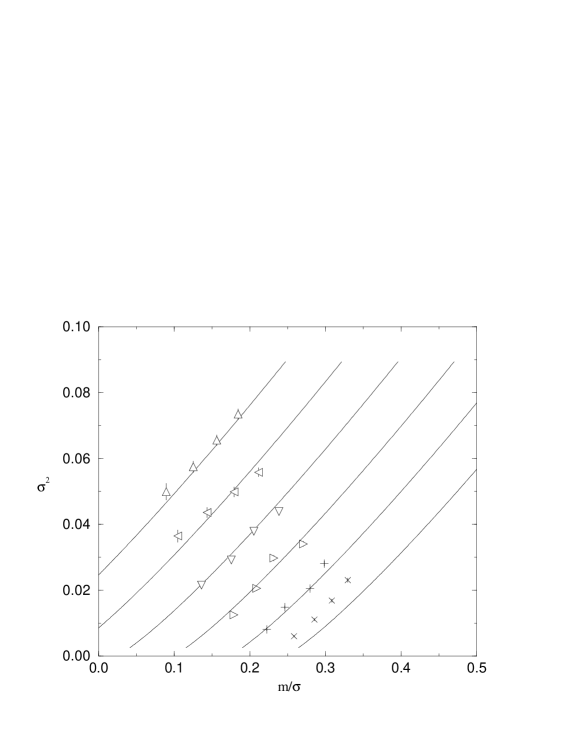
Figure 4: Fisher plot for $N_{f}=2$ on $12^{3}$ lattice. Values of $1/g^{2}$ range from 1.6 ($\triangle$) in steps of 0.2 to 2.6 ($\times$).

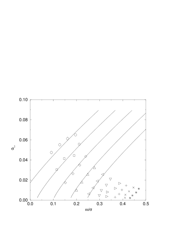
Figure 5: Fisher plot for $N_{f}=4$ on $12^{3}$ lattice. Values of $1/g^{2}$ range from 0.5 ($\bigcirc$) in steps of 0.1 to 1.4 ($\ast$).

In Figs. 4 and 5 we show the Fisher plots for $N_{f}=2,4$ on the $12^{3}$ lattice, together with the curves obtained using the parameters of fit II. The existence of a critical point separating a chirally symmetric phase from a phase where chiral symmetry is spontaneously broken can be easily spotted from the figures according to the above criterion. The corresponding lattice data can be fitted to the equation of state, yielding stable results and reasonably small $\chi^{2}$. The detailed results from the fits are reported in Tabs. 6 and 7. Fits I and II agree within errors for both values of $N_{f}$ on the $12^{3}$ lattice, justifying the use of the fit with the reduced number of parameters. From a practical point of view, such a justification becomes very important since a smaller number of variables is more easily fitted from the relatively small datasets that one can produce when dealing with dynamical fermions. In the following the results quoted will always be the ones from fit II, unless specified. The critical coupling $g_{c}$ does not seem to be unduly affected by finite-size effects, as one can see by comparing the results in Tab. 6, 7. The values extracted from the $12^{3}$ data for $N_{f}=2,4$ can thus be used to check the SD prediction of equation (1.9):

$$\frac{g^{2}_{c}(N_{f}=2)}{g^{2}_{c}(N_{f}=4)}=0.291$$ (3.13)

Comparing with our result

$$\frac{g^{2}_{c}(N_{f}=2)}{g^{2}_{c}(N_{f}=4)}=0.342\pm 0.015$$ (3.14)

we can conclude that the above prediction is more than three standard deviations away from the lattice data. This seems to favour the scenario where a critical number of flavors $N_{fc}$, exists. For $N_{f}>N_{fc}$ the theory would then be chirally symmetric for any value of the coupling. This conjecture is also supported by our data for $N_{f}=6$, shown in Fig. 6, where it is very difficult to identify a critical point corresponding to a symmetry breaking phase transition. Qualitatively as $g$ increases the trajectories seem to be accumulating around a line which if continued would intercept the horizontal axis. Quantitatively, neither fit I nor fit II provides a satisfactory description of the data. It is interesting to note that, in all the cases where the fit converged, the critical exponent $\delta$ is at least two standard deviations away from the mean field value $\delta=3$. Finally, let us remark that finite-size effects influence the value of the critical exponent $\delta$: the next sub–section is dedicated to the inclusion of these effects in our equation of state, so that the exponents extracted by our fitting procedure are those corresponding to the thermodynamic limit.

3.2 Finite size scaling and the equation of state

Finite size effects can be used to extract further information about the nature of the critical point. In the usual approach to finite size scaling, the RGE are assumed to be completely insensitive to finite size effects, since renormalisation deals with the short distance properties of the theory; they are therefore unchanged in a finite geometry. Nonetheless the finiteness of the volume affects the solutions of RGE, which now depend on one more dimensionful parameter. This is equivalent to considering the inverse linear size of the lattice, $1/L$, as an additional relevant scaling field with eigenvalue $1$ close to a fixed point at $L\rightarrow\infty$. By repeating the arguments explained above, we obtain an equation expressing the external field as a universal function of two rescaled variables:

$$m\langle\bar{\chi}\chi\rangle^{-\delta}\sim{\cal F}(tM^{-1/\beta},L^{-1/\nu}\langle\bar{\chi}\chi\rangle^{-1/\beta})$$ (3.15)

which can again be expanded to yield a new equation of state,

$$m=B\langle\bar{\chi}\chi\rangle^{\delta}+A(t+CL^{-1/\nu})\langle\bar{\chi}\chi\rangle^{\delta-1/\beta}+\mbox{higher order terms},$$ (3.16)

to which the data can be fitted, in principle allowing the extraction of three critical exponents ($\delta$, $\beta$ and $\nu$) and the critical coupling, taking into account finite size effects. The parameters obtained from this fit are the thermodynamic (infinite volume) limit ones. Hence, assuming the existence of a UV fixed point, the fit to this new equation of state provides a method to determine the thermodynamic limit of the critical exponents and coupling without further hypothesis.

Once again, it is important to stress that Eq. (3.16) is based on a Taylor expansion and is expected to describe the behaviour of the data only in a restricted region around the fixed point. As in the previous section, the set of data included in the fit is selected by maximising the $\chi^{2}$/d.o.f. In order to reduce the number of parameters in the fit, $\delta-1/\beta$ is set to 1 again and $\nu$ is assumed to obey the hyperscaling relation (3.9), as it should be in the vicinity of a RG fixed point so that $\nu=(\delta+1)/3(\delta-1)$. The number of parameters is then reduced from seven to five. Data from lattice sizes ranging from 8 to 16 have been included in the fit, whose results are reported in Tab. 8. It is clear from the values of the critical exponents that the theory is not mean-field and that the data around the critical point seem to match well the expected behaviour of a UV fixed point.

The data for the chiral condensate vs. $1/g^{2}$ are reported in Fig. 7 and 8 for the $12^{3}$ and $16^{3}$ lattices respectively, together with the curves obtained from the fit. The dashed line represents the chiral condensate for $m=0$ in the thermodynamic limit.

To conclude, in this section we have shown that the chiral condensate data of the $N_{f}=2$ and $N_{f}=4$ models support the hypothesis of a power-law equation of state in the critical region. The fits obtained were also consistent with the constraint $\delta-1/\beta=1$. In passing it is worth remarking that it is not possible to obtain a good fit to our data with a mean-field equation of state with logarithmic corrections, as used for ${\rm QED}_{4}$ in [35]. The critical exponents extracted for the two models are distinct, in neither case resembling those of mean field theory, suggesting that the two models have continuum limits described by distinct field theories. Of course, this in itself is not direct evidence for an interacting continuum limit at the fixed point; to establish that would require the study of lines of constant physics in the space of bare parameters $g$ and $m$, and measurement of $n$-point functions in the critical region. No similar fit was found for $N_{f}=6$, suggesting that in this case there is no transition, and that $N_{fc}<6$ for the Thirring model.

4 Susceptibilities and Spectroscopy

In this section we review results of susceptibility and spectroscopy measurements, principally on the $N_{f}=2$ model studied on a $16^{3}$ lattice with $m=0.01$ (ie. unless stated otherwise), but also showing some results from a smaller lattice, and for $N_{f}=4$, for comparison. First we consider susceptibilities, generically denoted $\chi$, which as discussed in Sec. 2 are equivalent to bound state propagators evaluated at zero three-momentum. They take large values whenever there are long-range correlations present. There are two reasons why $\chi$ is a useful quantity to study. Firstly, it can be separated into singlet $\chi_{s}$ and non-singlet $\chi_{ns}$ components; $\chi_{s}$, formed from disconnected valence fermion lines, is thus a useful measure of the importance of sea fermion loops in the vacuum. Since there are no dynamical bosons in the original model, any long-range interactions must be mediated by fermion “bubbles”. The relative strength of $\chi_{s}$ versus $\chi_{ns}$ is the simplest probe of this effect. Secondly, if we assume that fermion – anti-fermion composites resemble canonical bosons, then the relation

$$\chi={Z\over M^{2}}$$ (4.1)

holds, where $M$ is the bound state mass and $Z$ is a renormalisation constant associated with the projection of the composite operator onto the propagating state. Hence a large susceptibility signals a small bound state mass. However, in a non-confining theory the assumptions leading to (4.1) may not be justified, eg. when there is a contribution from the fermion – anti-fermion continuum as in the scalar channel of the three dimensional GN model [3]. In this case extraction of the bound-state mass is model dependent, whereas the susceptibility is still unambiguously defined.

First we consider the scalar channel, plotting in Fig. 9 $\chi_{ls}$, $\chi_{lns}$, and $\chi_{l}$ versus $1/g^{2}$ (see Eq. (2)). In the symmetric phase the signal is dominated by $\chi_{lns}$, which peaks at $1/g^{2}\sim 2\;-\;2.2$, indicating a possible light scalar state, before falling away in the broken phase. The singlet contribution is almost absent in the symmetric phase, but rises across the transition to dominate the signal by $1/g^{2}=1.6$. The total longitudinal susceptibility is approximately constant in the broken phase.

Next we compare longitudinal and transverse susceptibilities (2,2), showing data for $N_{f}=2$, $m=0.01$ on a $16^{3}$ lattice in Fig.10 and for $N_{f}=4$, $m=0.02$ on a $12^{3}$ lattice in Fig. 11. The main features are that $\chi_{l}\simeq\chi_{t}$ deep in the symmetric phase, but that $\chi_{t}$ rises steeply in the broken phase corresponding to the appearance of a massless Goldstone pion. Note that the non-singlet contribution $\chi_{tns}$ saturates the full Ward identity result within errors; this is as expected since singlet – non-singlet degeneracy could only be lifted by an axial anomaly, which is absent both for staggered fermions and for three dimensions.

There is an interesting relation between the ratio $R$ of longitudinal to transverse susceptibilities and the critical scaling behaviour of the model, first noted in [22] and subsequently developed in [35]. Using the action (2.1) and the Ward identity (2), we have

$$R(m,g^{2})={\chi_{l}\over\chi_{t}}={m\over{\langle\bar{\chi}\chi\rangle}}{{\partial\langle\bar{\chi}\chi\rangle}\over{\partial m}}.$$ (4.2)

Therefore $R$ can be calculated using the proposed equation of state (3.11):

$$R(m,g^{2})={1\over{\left(\delta-{\displaystyle 1\over\displaystyle\beta}\right)+{\displaystyle{B\langle\bar{\chi}\chi\rangle^{\delta}}\over\displaystyle{\beta m}}}}.$$ (4.3)

In general $R$ depends on $m$, but its limiting forms in the chiral limit are easily evaluated. In the broken phase, $\langle\bar{\chi}\chi\rangle$ remains non-vanishing in the chiral limit, whereas in the symmetric phase $\langle\bar{\chi}\chi\rangle^{\delta}$ vanishes faster than $m$; hence

$$\displaystyle\lim_{m\to 0}R=\cases{0,&$g^{2}>g_{c}^{2}$;\cr{1\over{\delta-{1\over\beta}}},&$g^{2}<g_{c}^{2}$.\cr}$$ (4.4)

The near-degeneracy of $\chi_{l}$ and $\chi_{t}$ in the symmetric phase from $1/g^{2}=2.4$ onwards seen in Fig. 10, and from $1/g^{2}=1.2$ onwards in Fig. 11, therefore provides additional support for our preferred value of $\delta-1/\beta=1$ in the equation of state (3.11). Exactly at the critical coupling, however, $R$ becomes independent of $m$, and we have

$$R|_{g=g_{c}}={1\over\delta}.$$ (4.5)

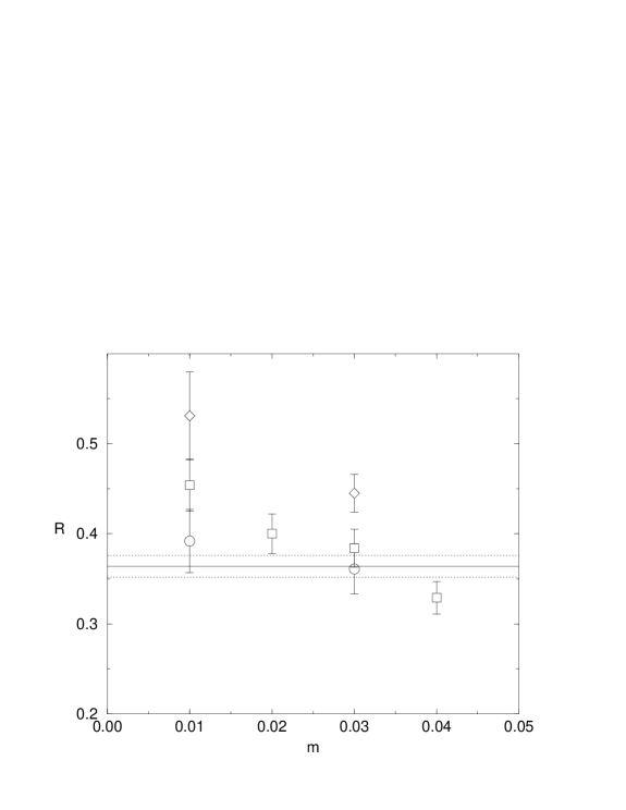
Figure 12: Susceptibility ratio $R$ vs. $m$ for $1/g^{2}=1.9$ (circles), 1.92 (squares) and 2.0 (diamonds). The horizontal band marks the value of $1/\delta$ from the fit (3.16).

In Tab. 9 and Fig. 12 we plot $R$ for various values of $m$ and $g$ near the critical point, in particular for four values of $m$ evaluated at our best estimate of the critical coupling $1/g^{2}=1.92$. It is worth noting that the ratio $\chi_{ls}/\chi_{lns}$ exceeds 40% in this region, showing the importance of including the disconnected contributions in this particular calculation. However, we also find that $R$ decreases significantly with $m$, at first sight implying that the model is in the symmetric phase at this coupling; the variation of $R$ with $m$ is less pronounced at $1/g^{2}=1.90$, which would thus appear to be closer to the critical coupling. This apparent contradiction is resolved if we take the finite-size scaling form (3.16) seriously. Using the fit parameters from Tab. 8 the coefficient multiplying the $\langle\bar{\chi}\chi\rangle^{\delta-1/\beta}$ term actually vanishes for $1/g^{2}\simeq 1.88$. We should therefore expect to observe a constant $R$ at slightly stronger couplings than the critical one on a finite system. Although we have insufficient data to verify this directly, it is clear that this kind of analysis has the potential to provide an independent estimate of $g_{c}^{2}$ and $\delta$. An optimistic reader would consider the near-agreement found here as a signal of the fact that the RG structure underlying the equation of state approach is indeed realised in the Thirring model.

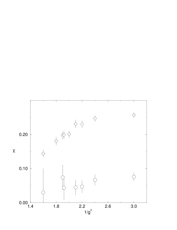
Figure 13: Vector susceptibilities $\chi_{vs}$ (circles) and $\chi_{vns}$ (diamonds) vs. $1/g^{2}$.

In Fig. 13 we plot the vector susceptibilities $\chi_{vs}$ and $\chi_{vns}$ (2). The data is quite noisy; the trends are that $\chi_{vns}$ appears roughly constant in the symmetric phase and fall away in the broken phase, and that the ratio $\chi_{vs}/\chi_{vns}$ lies between 0.2 and 0.3 throughout the region.

Next we discuss spectroscopy, which involves the calculation of the timesliced correlators $C(t)$ defined in Sec. 2. We follow the usual procedure of extracting the mass of the lowest–lying state contributing to the two–point functions from their single exponential decay for large time separations. In performing our minimum $\chi^{2}$ fits, we include correlations between the data at different timeslices. We used the bootstrap technique to estimate errors on the fitted parameters. We present results from $8^{2}\times 16$ and $16^{3}$ lattices.

First consider the fermion, pion and scalar channels. The fermion, since it cannot mix with any excited states, shows the clearest signal and can be fitted over the entire range by the form

$$C_{f}(t)=A\left(e^{-\mu_{R}t}-(-1)^{t}e^{-\mu_{R}(L-t)}\right),$$ (4.6)

where $\mu_{R}$ is the physical fermion mass and the minus sign between the forward and backward terms is due to our choice of antiperiodic boundary conditions in the timelike direction. All the quoted results are obtained from fitting in the range $t\in[2,13]$ with a typical $\chi^{2}$/dof $\sim 1$. Varying the fit range produces negligible variations in the fitted parameters and $\chi^{2}$/dof.

Both the scalar and pion channels were fitted by the form

$$C_{l}(t)=A\left(e^{-Mt}+e^{-M(L-t)}\right).$$ (4.7)

The pion exhibits single exponential decay from early timeslices and it is possible to fit the data in the range $t\in[3,13]$ in almost all cases, again with a typical $\chi^{2}/\mbox{dof}\sim 1$. Similarly to the fermion case, fitting over a smaller time interval within this range produces minimal variations. The scalar channel is more problematic. Firstly the signals exhibit greater statistical noise. Secondly, as distinct from the pion channel, we can only fit the correlators in a restricted time interval, suggesting contamination of the signal by higher-mass states. On the $8^{2}\times 16$ lattice it is not possible to reliably extract the ground-state signal for $m=0.05$, while for $m=0.02$, fits are possible but quite sensitive to the fitted range. In this latter case we therefore choose a conservative fit range $t\in[4,11]$; fitting outside this range leads to a much higher $\chi^{2}$/dof. The fits on the $16^{3}$ data are more stable for all values of the fermion bare mass. In the strong coupling regime, where the scalar mass gets larger, it proves harder to extract the ground–state mass regardless of bare mass or lattice size, resulting in larger errors on the fitted masses in this phase. In order to improve on this behaviour, it would be necessary to move to larger lattices. With regard to this last point, our present results should therefore be considered as an attempt to find qualitative evidence of the phase structure of the model, rather than a precise evaluation of its spectrum. The detailed results are presented in Tabs. 10, 11, 12, 13 and 14. Examples of the fermion, pion and scalar signals are shown in Figs. 14, 15 and 16 respectively.

A comparison between Tabs. 11 and 13 enables a crude assessment of finite volume effects. In the smaller volume the fermion mass $\mu_{R}$ is shifted upwards significantly in the symmetric phase, while remaining relatively unaffected, within errors, deep in the broken phase. The pion, in contrast, is lighter in the smaller volume, the effect again being more pronounced in the symmetric phase, but still significant in the broken phase. The scalar mass seems the least affected by the finite volume.

In Fig. 17 we plot the measured masses against $1/g^{2}$ for the $16^{3}$ system at $m=0.01$. While the pion mass stays constant, the fermion mass is small in the symmetric phase, but rises steeply across the transition to become heavier than the pion in the broken phase. Just on the symmetric side of the transition we have $M_{\pi}\simeq 2\mu_{R}$, indicating that the pion is a weakly bound state – unfortunately by $1/g^{2}=2.4$ this picture breaks down, perhaps due to finite volume effects. The scalar mass, meanwhile, is just greater but of the same order as the pion mass in the symmetric phase, but rises across the transition to become appreciably larger. The scalar and pion masses are respectively related to the longitudinal and transverse susceptibilities:

$$\chi_{l,t}=Z_{s,\pi}/M^{2}_{s,\pi}$$ (4.8)

The chiral Ward identity (2) then yields:

$$M^{2}_{\pi}=\frac{Z_{\pi}}{\langle\bar{\chi}\chi\rangle}m.$$ (4.9)

As long as chiral symmetry is broken, this equation states that the pion mass squared is a linear function of the bare mass and hence vanishes when the breaking is dynamical (Goldstone theorem). Fig. 18 shows the behaviour of the pion mass squared as $m\rightarrow 0$ in the broken phase for $1/g^{2}=1.8$. The line is a least squares fit; the fitted intercept lies two standard deviations from the origin, which is another signal of systematic error.

It is satisfying that the spectrum reflects the phase transition so sharply, moreover in a manner entirely consistent with standard expectations – there is no evidence for the unconventional spectrum in the symmetric phase, associated with an infinite order phase transition, discussed in [15]. Of course, it would be valuable to refine this initial study both by working closer to the chiral limit, and with more lattice spacings in the timelike direction to improve the mass estimates – clearly at present we are unable to make reliable estimates of binding energies, and hence are unable to make detailed comparisons with the predictions of the $1/N_{f}$ expansion in the symmetric phase.

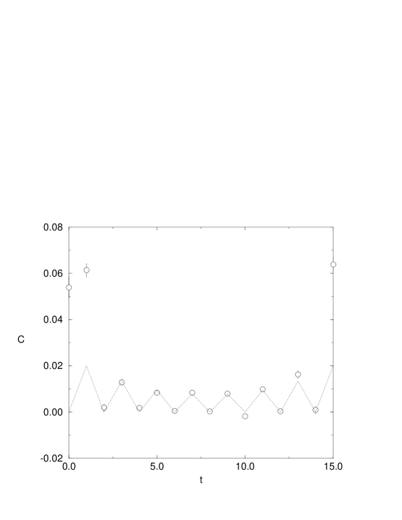
Figure 19: Conserved vector correlator, plus 2 parameter fit, at $1/g^{2}=2.4$.

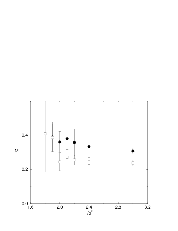
Figure 20: Local (circles) and conserved (squares) vector masses from 2 parameter fit vs. $1/g^{2}$.

Finally we turn to the vector channels, where we have employed both local (2.33) and one-link “conserved” (2.34) interpolating operators. In either case we found that the signal had a strong alternating component, exemplified by the plot shown in Fig. 19. Therefore fits of the form (2.35) were used. Superficially, the main difference between the two different vector channels was that the local vector gave numerically larger but noisier signals. For both operators we experimented with two parameter fits, with $B$ set equal to $-A$ and $M_{d}$ equal to $M_{a}$ in (2.35) for $t\in[3,13]$, then three parameter fits in which $A$ and $B$ are allowed to differ, and finally the most general four parameter fit in which $A$, $B$, $M_{d}$ and $M_{a}$ are all independent, the last two forms being fitted for $t\in[2,14]$. The results are summarised in Tabs. 15, 16, and plotted in Fig.  20.

The main trends we found are:

(i) For all fits the mass of the local operator lies significantly above that of the conserved operator. This should be no surprise, since as discussed in Sec. 2, and displayed in Tab. 5, the two operators have different quantum numbers in three dimensions.

(ii) The masses are approximately constant throughout the symmetric phase; across the transition the signal becomes smaller and thus noisier, consistent with the falloff in $\chi_{vns}$ of Fig. 13. Our mass fits are of limited use for $1/g^{2}\leq 1.8$. In the conserved channel, however, there is evidence for a sharp rise in mass at $1/g^{2}=1.9$. Hence there may be a light vector particle in the symmetric phase, in accordance with the $1/N_{f}$ expansion, but not in the broken phase.

(iii) Although the two parameter fits gave acceptable results, there is tentative evidence in the conserved channel that the four parameter fit is significantly better, with $M_{a}<M_{d}$, particularly from the results with $m=0.02$ at $1/g^{2}=2.4$. An examination of Tab. 5 reveals that the direct channel has the vector spin quantum number form $\bar{\psi}\gamma_{\mu}\psi$ while the alternating channel has the “axial vector” form $\bar{\psi}\gamma_{5}\gamma_{\mu}\psi$. Inspection of the lattice interaction in the form (2.12) shows that there is a contact interaction between axial vector currents of equal strength to that between vector currents; therefore it is reasonable that the one-link operator projects onto both states with comparable strengths, resulting in $C(t)$ almost vanishing on even timeslices (Fig. 19). Thus we find both light vectors and light axial vectors in the symmetric phase. We have no explanation for the light axial vector. Following the analysis of [8], we can examine the pole condition $p^{2}=-M_{A}^{2}$ in the axial vector channel to leading order in $1/N_{f}$:

$$1+{g^{2}\over{2\pi}}\left[m+{{4m^{2}-M_{A}^{2}}\over{4M_{A}}}\ln\left({{2m+M_{A}}\over{2m-M_{A}}}\right)\right]=0.$$ (4.10)

One readily sees that this equation has no bound state solution of the form $M_{A}=2m-\varepsilon$. It would be interesting to see whether this persists at next-to-leading order in $1/N_{f}$.

To summarise, the results in the vector channel present the only unexpected result; the light state in the axial vector channel is the first hint of departure from behaviour predicted by the $1/N_{f}$ expansion in the symmetric phase. In future studies at smaller bare fermion masses, it would be interesting to monitor the ratio $\chi_{vs}/\chi_{vns}$, to see whether the channel becomes dominated by fermion bubble chains as in the $1/N_{f}$ expansion. It would also be interesting to repeat this analysis in simulations of non-compact lattice $\mbox{QED}_{3}$ to see whether the light axial vector is present or not – in this case since the $A_{\mu}$ field is now a dynamical variable, it is possible that short-wavelength fluctuations will be suppressed by a factor $1/k^{2}$, preventing the strong coupling to the axial vector channel occurring in (2.12).

5 Conclusions

In conclusion we briefly summarise our main findings, and suggest further directions to explore. For $N_{f}=2$ and $N_{f}=4$ the Thirring model exhibits a phase transition at finite critical coupling $g^{2}_{c}$ to a phase in which chiral symmetry is spontaneously broken. This contradicts the naive $1/N_{f}$ expansion, but supports the predictions of non-perturbative methods such as the Schwinger-Dyson approach. In the vicinity of the critical point the model’s equation of state seems well fitted by a renormalisation-group inspired form corresponding to power-law scaling. The picture remains consistent for $N_{f}=2$ even once a finite volume scaling analysis, using data from larger lattices and smaller bare masses, is employed. The critical exponents we find differ significantly between $N_{f}=2$ and $N_{f}=4$, suggesting that the two models lie in different universality classes. Although it is tempting to infer the existence of non-perturbative continuum limits at these points, it would be nice to have direct evidence by measurement of a renormalised coupling constant via a 3- or 4-point correlation function.

For $N_{f}=6$ the picture is not so clear, and we did not find a fixed-point fit for the equation of state. The Fisher plot of Fig. 6 strongly suggests that in the chiral limit the model lies in the symmetric phase for all values of the coupling, and hence that $N_{fc}<6$. However, bearing in mind the practical difficulties in identifying the strong coupling limit discussed in Sec. 2, perhaps a more conservative conclusion is that the $N_{f}=6$ model seems qualitatively very different from $N_{f}=2,4$ [33]. It might be very difficult ever to exclude absolutely a chiral condensate exponentially suppressed in $N_{f}$ for large $N_{f}$; however our data disagrees with the only theoretical prediction (1.9) to put forward this scenario [11]. We intend to extend the $N_{f}=6$ studies to larger lattices and smaller $m$ to pursue this issue further.

Although we made no attempt to test the scaling form (1.8), corresponding to an infinite order phase transition, our studies of the susceptibilities and spectrum prejudice us against this scenario: the relative ordering of the physical fermion, scalar and pseudoscalar masses varies continuously across the transition; there appear to be light bound states in the symmetric phase, comparable with the scale set by the physical fermion mass, in contradiction to the behaviour expected near a conformal transition discussed in Refs. [15, 16]. It would be interesting to extend this study to $N_{f}=4$, where $g_{c}$ lies closer to the strong coupling limit, to see if the spectrum shows any qualitative difference. Work in this direction is in progress.

Finally, although our admittedly exploratory spectrum analysis has yielded important information, it is clear that larger lattices in the timelike direction will be needed before accurate measurements of masses and binding energies, or indeed departures from the exponential form of the decay corresponding to a spectral function more complicated than simple isolated poles, can be accomplished. Accurate mass measurements would be desirable in order to compare with predictions from the $1/N_{f}$ expansion, to check whether the latter approach has any validity near the transition even in the symmetric phase. There is a first hint of its breaking down in the apparent existence of a light axial vector state here; however it is clear much more work is needed both numerically and analytically.

6 Acknowledgements

LDD is supported by an EU HCM Institutional Fellowship, SJH by a PPARC Advanced Fellowship. Some of the computing work was performed using resources made available under PPARC research grant GR/J67475, and those of the UKQCD collaboration under GR/K41663, GR/K455745 and GR/L29927. We have enjoyed discussing aspects of this work with Roger Horsley, Yoonbai Kim, Kei-Ichi Kondo and Nick Mavromatos.

Table 1: List of results for the chiral condensate for $N_{f}=2$

$L$	$m$	$1/g^{2}$	$\langle\bar{\chi}\chi\rangle$	$\Delta\langle\bar{\chi}\chi\rangle$
8	0.01	1.8	0.08610	0.0030
8	0.01	2.0	0.06130	0.0020
8	0.01	2.2	0.05170	0.0020
8	0.01	2.4	0.00425	0.0010
8	0.02	0.5	0.25097	0.0084
8	0.02	1.0	0.28171	0.0110
8	0.02	1.5	0.20172	0.0068
8	0.05	1.6	0.26956	0.0080
8	0.05	1.8	0.22639	0.0060
8	0.05	2.0	0.20417	0.0040
8	0.05	2.2	0.18051	0.0043
8	0.05	2.4	0.15785	0.0038
8	0.05	2.6	0.14403	0.0035
8	0.05	2.8	0.13393	0.0028
12	0.01	1.6	0.17485	0.0057
12	0.02	1.6	0.22341	0.0055
12	0.02	1.8	0.19083	0.0047
12	0.02	2.0	0.14680	0.0040
12	0.02	2.2	0.11172	0.0026
12	0.02	2.4	0.08992	0.0020
12	0.02	2.6	0.07737	0.0015
12	0.02	2.8	0.06493	0.0010
12	0.02	3.0	0.05715	0.0008
12	0.02	3.2	0.05256	0.0007
12	0.02	3.4	0.04784	0.0006
12	0.03	1.6	0.23970	0.0035
12	0.03	1.8	0.20873	0.0036
12	0.03	2.0	0.17070	0.0023
12	0.03	2.2	0.14342	0.0025
12	0.03	2.4	0.12171	0.0017
12	0.03	2.6	0.10508	0.0013
12	0.03	2.8	0.09153	0.0011
12	0.03	3.0	0.08303	0.0008
12	0.03	3.2	0.07554	0.0008
12	0.03	3.4	0.07107	0.0007

Table 2: List of results for $N_{f}=2$ (continued)

$L$	$m$	$1/g^{2}$	$\langle\bar{\chi}\chi\rangle$	$\Delta\langle\bar{\chi}\chi\rangle$
12	0.04	1.6	0.25599	0.0031
12	0.04	1.8	0.22321	0.0032
12	0.04	2.0	0.19460	0.0030
12	0.04	2.2	0.17244	0.0024
12	0.04	2.4	0.14307	0.0019
12	0.04	2.6	0.12966	0.0018
12	0.04	2.8	0.11604	0.0015
12	0.04	3.0	0.10851	0.0012
12	0.04	3.2	0.09707	0.0011
12	0.04	3.4	0.09282	0.0008
12	0.05	1.6	0.27098	0.0030
12	0.05	1.8	0.23624	0.0028
12	0.05	2.0	0.20952	0.0025
12	0.05	2.2	0.18450	0.0020
12	0.05	2.4	0.16750	0.0020
12	0.05	2.6	0.15171	0.0020
12	0.05	2.8	0.13861	0.0014
12	0.05	3.0	0.12572	0.0012
12	0.05	3.2	0.11861	0.0011
12	0.05	3.4	0.11118	0.0010
16	0.01	1.6	0.20250	0.0028
16	0.01	1.8	0.14190	0.0021
16	0.01	1.9	0.12780	0.0032
16	0.01	1.92	0.12419	0.0018
16	0.01	2.0	0.10250	0.0021
16	0.01	2.1	0.08614	0.0020
16	0.01	2.2	0.07177	0.0012
16	0.01	2.4	0.05287	0.0010
16	0.02	1.6	0.22040	0.0030
16	0.02	1.92	0.15733	0.0013
16	0.02	2.0	0.14580	0.0012
16	0.02	2.4	0.09430	0.0006
16	0.03	1.8	0.20440	0.0010
16	0.03	1.9	0.18624	0.0009
16	0.03	1.92	0.18547	0.0010
16	0.03	2.0	0.17174	0.0009
16	0.03	2.1	0.15632	0.0009
16	0.04	1.92	0.20576	0.0008

Table 3: List of results for $N_{f}=4$

$L$	$m$	$1/g^{2}$	$\langle\bar{\chi}\chi\rangle$	$\Delta\langle\bar{\chi}\chi\rangle$
12	0.02	0.6	0.21771	0.0037
12	0.02	0.7	0.17435	0.0032
12	0.02	0.8	0.13163	0.0030
12	0.02	0.9	0.09994	0.0024
12	0.02	1.0	0.07917	0.0018
12	0.02	1.1	0.06700	0.0011
12	0.02	1.2	0.06030	0.0008
12	0.02	1.3	0.05453	0.0007
12	0.02	1.4	0.04882	0.0005
12	0.02	1.5	0.04636	0.0005
12	0.03	0.6	0.23476	0.0033
12	0.03	0.7	0.20343	0.0031
12	0.03	0.8	0.16221	0.0028
12	0.03	0.9	0.13419	0.0020
12	0.03	1.0	0.11065	0.0017
12	0.03	1.1	0.09750	0.0020
12	0.03	1.2	0.08977	0.0016
12	0.03	1.3	0.07804	0.0009
12	0.03	1.4	0.07295	0.0009
12	0.03	1.5	0.06793	0.0006
12	0.04	0.6	0.24741	0.0036
12	0.04	0.7	0.21080	0.0028
12	0.04	0.8	0.18680	0.0024
12	0.04	0.9	0.16079	0.0030
12	0.04	1.0	0.13808	0.0020
12	0.04	1.1	0.12140	0.0018
12	0.04	1.2	0.10850	0.0013
12	0.04	1.3	0.10094	0.0010
12	0.04	1.4	0.09362	0.0009
12	0.04	1.5	0.08734	0.0008
12	0.05	0.6	0.25489	0.0026
12	0.05	0.7	0.23618	0.0025
12	0.05	0.8	0.20854	0.0022
12	0.05	0.9	0.18000	0.0021
12	0.05	1.0	0.160	0.0016
12	0.05	1.1	0.14423	0.0015
12	0.05	1.2	0.12921	0.0013
12	0.05	1.3	0.12051	0.0012
12	0.05	1.4	0.11202	0.0011
12	0.05	1.5	0.10653	0.0010

Table 4: List of results for $N_{f}=6$

$L$	$m$	$1/g^{2}$	$\langle\bar{\chi}\chi\rangle$	$\Delta\langle\bar{\chi}\chi\rangle$
12	0.02	0.25	0.14342	0.0034
12	0.02	0.3	0.14687	0.0035
12	0.02	0.35	0.13924	0.0040
12	0.02	0.4	0.11832	0.0030
12	0.02	0.45	0.09867	0.0040
12	0.02	0.5	0.07608	0.0020
12	0.03	0.25	0.16721	0.0030
12	0.03	0.3	0.17836	0.0040
12	0.03	0.35	0.17099	0.0032
12	0.03	0.4	0.15218	0.0028
12	0.03	0.45	0.12766	0.0030
12	0.03	0.5	0.10716	0.0020
12	0.04	0.3	0.18403	0.0029
12	0.04	0.35	0.18659	0.0031
12	0.04	0.4	0.17549	0.0026
12	0.04	0.45	0.15650	0.0022
12	0.04	0.5	0.13959	0.0038
12	0.05	0.25	0.19691	0.0028
12	0.05	0.3	0.20373	0.0029
12	0.05	0.35	0.20636	0.0028
12	0.05	0.4	0.19784	0.0030
12	0.05	0.45	0.17549	0.0017
12	0.05	0.5	0.15903	0.0020

Table 5: Spin/flavor assignments of the fermion bilinears used in spectroscopy

	direct	alternating
pion	$\gamma_{5}\otimes 1\kern-4.5pt1$	$\gamma_{\mu}\gamma_{\nu}\otimes\tau_{\mu}^{*}\tau_{\nu}^{*}$
scalar	$1\kern-4.5pt1\otimes 1\kern-4.5pt1$	$\gamma_{5}\gamma_{\mu}\gamma_{\nu}\otimes\tau_{\mu}^{*}\tau_{\nu}^{*}$
local vector	$\gamma_{\mu}\gamma_{3}\otimes\tau_{3}^{*}\tau_{\mu}^{*}$	$\gamma_{5}\gamma_{\mu}\gamma_{3}\otimes\tau_{3}^{*}\tau_{\mu}^{*}$
conserved vector	$\gamma_{\mu}\otimes 1\kern-4.5pt1$	$\gamma_{5}\gamma_{\mu}\otimes\tau_{3}^{*}$

Table 6: Results from fits on the $12^{3}$ lattice.

	Parameter	Fit I	Fit II
$N_{f}=2$	$1/g^{2}_{c}$	2.03(9)	1.94(4)
	$\delta$	2.32(23)	2.68(16)
	$\beta$	0.71(9)	—
	$A$	0.32(5)	0.37(1)
	$B$	1.91(43)	2.86(35)
	$\chi^{2}$/d.o.f	2.4	2.1
$N_{f}=4$	$1/g^{2}_{c}$	0.63(1)	0.66(1)
	$\delta$	3.67(28)	3.43(19)
	$\beta$	0.38(4)	—
	$A$	0.78(5)	0.73(2)
	$B$	7.9(2.8)	6.4(1.5)
	$\chi^{2}$/d.o.f	3.1	2.0

Table 7: Results from fits on the $16^{3}$ lattice.

	Parameter	Fit I	Fit II
$N_{f}=2$	$1/g^{2}_{c}$		1.93(4)
	$\delta$		2.55(15)
	$\beta$		—
	$A$		0.38(1)
	$B$		2.29(35)
	$\chi^{2}$/d.o.f		2.3

Table 8: Results from fit including finite size scaling.

	Parameter	Fit III
$N_{f}=2$	$1/g^{2}_{c}$	1.92(2)
	$\delta$	2.75(9)
	$\beta$	0.57(2)
	$\eta$	0.60(2)
	$\nu$	0.71(4)
	$A$	0.334(7)
	$B$	2.7(3)
	$C$	2.1(7)
	$\chi^{2}$/d.o.f	1.76

Table 9: Longitudinal and transverse susceptibilities in the vicinity of the critical coupling.

$1/g^{2}$	$m$	$\chi_{ls}$	$\chi_{lns}$	$\chi_{l}$	$\chi_{t}$	$R=\chi_{l}/\chi_{t}$
1.9	0.01	1.51(15)	3.40(40)	4.90(43)	12.49(20)	0.392(35)
	0.03	0.57(8)	1.68(15)	2.24(17)	6.22(4)	0.361(28)
1.92	0.01	1.65(19)	3.88(28)	5.53(34)	12.17(25)	0.454(29)
	0.02	0.72(8)	2.41(15)	3.13(17)	7.83(7)	0.400(22)
	0.03	0.67(9)	1.70(10)	2.37(13)	6.17(5)	0.384(21)
	0.04	0.34(5)	1.35(8)	1.69(9)	5.15(3)	0.329(18)
2.0	0.01	1.13(19)	4.25(44)	5.37(48)	10.12(21)	0.531(49)
	0.03	0.62(8)	1.93(9)	2.54(12)	5.71(5)	0.445(21)

Table 10: Masses for the fermion, pion and scalar, $16^{3}$ lattice, $m=0.01$

$1/g^{2}$	$\mu_{R}$	$M_{\pi}$	$M_{s}$
1.6	0.36 (3)	0.20 (1)	—
1.8	0.23 (2)	0.23 (2)	0.47 (4)
1.9	0.16 (1)	0.21 (1)	0.33 (2)
2.0	0.10 (1)	0.24 (1)	0.29 (1)
2.1	0.10 (1)	0.22 (1)	0.27 (1)
2.2	0.08 (1)	0.21 (1)	0.26 (1)
2.4	0.06 (1)	0.21 (1)	0.23 (1)

Table 11: Masses for the fermion, pion and scalar, $16^{3}$ lattice, $m=0.02$

$1/g^{2}$	$\mu_{R}$	$M_{\pi}$	$M_{s}$
1.6	0.330 (40)	0.280 (4)	0.52 (15)
1.8	0.360 (40)	0.290 (6)	0.39 (8)
1.92	0.200 (10)	0.280 (4)	0.43 (6)
2.0	0.190 (10)	0.300 (5)	0.35 (5)
2.4	0.109 (3)	0.290 (4)	0.27 (1)

Table 12: Masses for the fermion, pion and scalar, $16^{3}$ lattice, $m=0.03$

$1/g^{2}$	$\mu_{R}$	$M_{\pi}$	$M_{s}$
1.8	0.290 (20)	0.340 (5)	0.64 (9)
1.9	0.240 (20)	0.338 (4)	0.60 (4)
1.92	0.250 (20)	0.338 (4)	0.64 (6)
2.0	0.270 (20)	0.344 (4)	0.54 (4)
2.1	0.210 (10)	0.341 (4)	0.50 (3)

Table 13: Masses for the fermion, pion and scalar, $8^{2}\times 16$ lattice, $m=0.02$

$1/g^{2}$	$\mu_{R}$	$M_{\pi}$	$M_{s}$
1.6	****	****	****
1.7	0.340 (30)	0.256 (4)	0.42 (5)
1.9	0.290 (20)	0.240 (5)	0.44 (7)
2.0	0.280 (10)	0.231 (6)	0.30 (7)
2.1	0.200 (10)	0.231 (6)	0.26 (3)
2.2	0.240 (10)	0.225 (5)	0.29 (2)
2.3	0.185 (5)	0.225 (6)	0.23 (2)
2.4	0.170 (9)	0.206 (5)	0.26 (2)

Table 14: Masses for the fermion, pion and scalar, $8^{2}\times 16$ lattice, $m=0.05$

$1/g^{2}$	$\mu_{R}$	$M_{\pi}$	$M_{s}$
1.6	0.480 (40)	0.398 (4)	—
1.7	0.470 (30)	0.390 (4)	—
1.8	—	0.390 (4)	—
1.9	0.350 (10)	0.386 (3)	—
2.0	0.350 (20)	0.378 (4)	—
2.1	0.320 (10)	0.368 (4)	—
2.2	0.280 (10)	0.362 (4)	—
2.3	—	0.359 (3)	—
2.4	0.255 (9)	0.349 (3)	—
2.5	0.246 (7)	0.340 (3)	—

Table 15: Masses obtained in the local vector channel from a $16^{3}$ lattice

# fitted parameters	$m$	$1/g^{2}$	$M_{d}$	$M_{a}$	$\chi^{2}$/dof
2	0.01	3.0	0.307(18)		7.1
		2.4	0.332(63)		1.4
		2.2	0.357(79)		4.2
		2.1	0.379(109)		1.2
		2.0	0.360(61)		1.7
		1.9	0.389(88)		0.4
		1.8	0.807(665)		2.3
	0.02	2.4	0.365(34)		4.2
	0.03	2.1	0.952(183)		3.7
		2.0	0.870(171)		2.6
		1.9	0.438(88)		2.5
		1.8	0.928(333)		1.5
3	0.01	3.0	0.310(19)		3.4
		2.4	0.350(57)		0.8
		2.2	0.388(67)		1.8
		2.1	0.479(132)		1.5
		2.0	0.358(59)		1.0
		1.9	0.397(87)		0.3
		1.8	0.764(495)		2.4
4	0.01	3.0	0.263(18)	0.256(19)	1.2
		2.4	0.309(57)	0.294(62)	0.7
		2.2	0.336(66)	0.284(100)	1.9
		2.1	0.448(106)	0.312(103)	1.1
		2.0	0.358(60)	0.345(79)	1.3
		1.9	0.395(100)	0.337(173)	0.5
		1.8	0.701(457)	1.368(2.7)	2.5

Table 16: Masses obtained in the conserved vector channel from a $16^{3}$ lattice

# fitted parameters	$m$	$1/g^{2}$	$M_{d}$	$M_{a}$	$\chi^{2}$/dof
2	0.01	3.0	0.237(18)		3.0
		2.4	0.259(30)		2.1
		2.2	0.255(29)		1.3
		2.1	0.271(45)		0.7
		2.0	0.244(53)		1.5
		1.9	0.386(80)		0.5
		1.8	0.409(224)		0.6
	0.02	2.4	0.306(18)		2.2
	0.03	2.1	0.489(45)		1.3
		2.0	0.656(75)		1.9
		1.9	0.566(114)		2.8
		1.8	0.814(218)		0.9
3	0.01	3.0	0.239(15)		2.8
		2.4	0.266(30)		1.9
		2.2	0.257(29)		1.5
		2.1	0.312(42)		0.5
		2.0	0.258(56)		1.8
		1.9	0.456(89)		0.9
		1.8	0.974(879)		0.9
4	0.01	3.0	0.253(18)	0.230(17)	2.9
		2.4	0.293(34)	0.229(36)	1.8
		2.2	0.325(37)	0.162(46)	0.5
		2.1	0.320(43)	0.259(73)	0.5
		2.0	0.302(63)	0.223(67)	1.9
		1.9	0.605(204)	0.190(203)	0.5
	0.02	2.4	0.366(20)	0.220(23)	1.2

Figure 1: $\beta$-function for $d=2$ and $2<d<4$, showing for the latter case a non-trivial UV fixed point and phase structure.

Figure 2: Diagrams contributing to vacuum polarisation in lattice QED.

Figure 6: Fisher plot for $N_{f}=6$ on $12^{3}$ lattice.

Figure 7: Chiral condensate vs. $1/g^{2}$ on $12^{3}$ lattice. The solid lines are the fits from (3.16), the dashed line the extrapolation to chiral and thermodynamic limits.

Figure 8: Chiral condensate vs. $1/g^{2}$ on $16^{3}$ lattice.

Figure 9: $\chi_{ls}$ (circles), $\chi_{nls}$ (squares) and $\chi_{l}$ (diamonds) vs. $1/g^{2}$.

Figure 10: $\chi_{t}$ (squares), $\chi_{tns}$ (triangles) and $\chi_{lns}$ (circles) vs. $1/g^{2}$ for $N_{f}=2$.

Figure 11: $\chi_{t}$ (squares), $\chi_{tns}$ (triangles) and $\chi_{lns}$ (circles) vs. $1/g^{2}$ for $N_{f}=4$.

Figure 14: Fermion correlator for $1/g^{2}=2.2$.

Figure 15: Pion correlator for $1/g^{2}=2.2$.

Figure 16: Scalar correlator for $1/g^{2}=2.2$.

Figure 17: Fermion (filled circles), pion (squares) and scalar (diamonds) masses vs. $1/g^{2}$.

Figure 18: $M_{\pi}^{2}$ vs. $m$ in the broken phase at $1/g^{2}=1.8$.

References

-
[1]
G. Parisi, Nucl. Phys. B 100 (1975) 368;
S. Hikami and T. Muta, Prog. Theor. Phys. 57 (1977) 785;
Z. Yang, Texas preprint UTTG-40-90 (1990). - [2] M. Gomes, R.S. Mendes, R.F. Ribeiro and A.J. da Silva, Phys. Rev. D 43 (1991) 3516.
- [3] S.J. Hands, A. Kocić and J.B. Kogut, Ann. Phys. 224 (1993) 29.
- [4] B. Rosenstein, B.J. Warr and S.H. Park, Phys. Rep. 205 (1991) 59.
- [5] L. Karkkainen, R. Lacaze, P. Lacock and B. Petersson, Nucl. Phys. B415 (1994) 781; erratum ibid B438 (1995) 650.
-
[6]
K.-I. Shizuya, Phys. Rev. D21 (1980)
2327;
J. Zinn-Justin, Nucl. Phys. B367 (1991) 105. - [7] T. Muta, Proceedings of the 1991 Nagoya Spring School on Dynamical Symmetry Breaking, ed. K. Yamawaki, World Scientific 1992.
- [8] S.J. Hands, Phys. Rev. D 51 (1995) 5816.
- [9] G. Gat, A. Kovner and B. Rosenstein, Nucl. Phys. B 385 (1992) 76.
-
[10]
D.Espriu, A. Palanques-Mestre, P. Pascual and R. Tarrach,
Z. Phys. C 13 (1982) 153;
A. Palanques-Mestre and P. Pascual, Comm. Math. Phys. 95 (1984) 277. - [11] D.K. Hong and S.H. Park, Phys. Rev. D 49 (1994) 5507.
- [12] T. Itoh, Y. Kim, M. Sugiura and K. Yamawaki, Prog. Theor. Phys. 93 (1995) 417.
- [13] T.W. Appelquist, M.J. Bowick, D. Karabali and L.C.R. Wijewardhana, Phys. Rev. D33 (1986) 3704; 3774.
-
[14]
P.I. Fomin, V.P. Gusynin, V.A. Miranskii and
Yu.A. Sitenko, Riv. Nuovo Cimento 6 (1983) 1;
V.A. Miranskii, Nuovo Cimento 90 A (1985) 149. - [15] V.A. Miranskii and K. Yamawaki, Nagoya preprint DPNU-96-58, hep-th/9611142 (1996).
- [16] T.W. Appelquist, J. Terning and L.C.R. Wijewardhana, Phys. Rev. Lett. 77 (1996) 1214.
- [17] K.-I. Kondo, Nucl. Phys. B 450 (1995) 251.
-
[18]
L. Del Debbio, S.J. Hands, Phys. Lett. B 373
(1996) 171
L. Del Debbio, talk presented at St. Louis Symposium on Lattice Field Theory, hep-lat/9608003 (1996). - [19] I.J.R. Aitchison and N.E. Mavromatos, Phys. Rev. B53 (1996) 9321.
-
[20]
M.R. Pennington and S.P. Webb, Brookhaven
preprint BNL-40886 (1988);
D. Atkinson, P.W. Johnson and M.R. Pennington, Brookhaven preprint BNL-41615 (1988);
M.R.Pennington and D. Walsh, Phys. Lett. B 253 (1991) 246. - [21] E. Dagotto, S.J. Hands, A. Kocić and J.B. Kogut, Nucl. Phys. B347 (1990) 217.
- [22] A. Kocić, J.B. Kogut and K.C. Wang, Nucl. Phys. B398 (1993) 405.
- [23] S.J. Hands, A. Kocić, J.B. Kogut, R.L. Renken, D.K. Sinclair and K.C. Wang, Nucl. Phys. B413 (1994) 503.
- [24] C.J. Burden and A.N. Burkitt, Europhys. Lett. 3 (1987) 545.
- [25] M.F.L. Golterman and J.Smit, Nucl. Phys. B245 (1984) 61.
- [26] M. Göckeler, private communication.
- [27] Y. Cohen, S. Elitzur and E. Rabinovici, Nucl. Phys. B220 (1983) 102.
-
[28]
Th. Jolicœur, Phys. Lett. B171 (1986) 143;
Th. Jolicœur, A. Morel and B. Petersson, Nucl. Phys. B274 (1986) 225. - [29] H.J. Rothe, Lattice Gauge Theories: An Introduction, ch. 13 (World Scientific, Singapore) (1992).
- [30] S.P. Booth, R.D. Kenway and B.J. Pendleton, Phys. Lett. B228 (1989) 115.
- [31] A. Ali Khan, M. Göckeler, R. Horsley, P.E.L. Rakow, G. Schierholz and H. Stüben, Phys. Rev. D51 (1995) 3751.
- [32] C. Frick and J. Jersák, Phys. Rev. D52 (1995) 340.
- [33] S. Kim and Y. Kim, Seoul preprint SNUTP-96-010, hep-lat/9605021 (1996).
- [34] J. Zinn-Justin, Quantum Field Theory and Critical Phenomena, ch. 25.6, (Oxford Science Publications) (1989).
- [35] M. Göckeler, R. Horsley, V. Linke, P.E.L. Rakow, G. Schierholz and H. Stüben, preprint DESY-96-084, hep-lat/9605035 (1996).