Topology of the SU(2) vacuum: a lattice study using improved cooling
Philippe de Forcrand^a, Margarita García Pérez^b
and
Ion-Olimpiu Stamatescu^c,b

^a SCSC, ETH-Zürich, CH-8092 Zürich, Switzerland.

^b Institut f. Theoretische Physik, University of Heidelberg,

D-69120 Heidelberg, Germany.

^c FEST, Schmeilweg 5, D-69118 Heidelberg, Germany.

Abstract: We study the topological structure of the SU(2) vacuum at zero temperature: topological susceptibility, size, shape and distance distributions of the instantons. We use a cooling algorithm based on an improved action with scale invariant instanton solutions. This algorithm needs no monitoring or calibration, has an inherent cut off for dislocations and leaves unchanged instantons at physical scales. The physical relevance of our results is checked by studying the scaling and finite volume dependence. We obtain a susceptibility of $(200(15){\rm MeV})^{4}$. The instanton size distribution is peaked around $0.43$fm, and the distance distribution indicates a homogeneous, random spatial structure.

1 Introduction

Much work has been devoted to the study of topology within the framework of lattice gauge theories. Among other topics the measurement of the topological susceptibility and investigations of the relevance of instantons to the QCD vacuum have attracted a lot of interest.

The topological susceptibility is a physical quantity which measures the fluctuations of the topological charge of the vacuum. It is related via the Witten-Veneziano formula [1, 2] to a phenomenological parameter (the $\eta^{\prime}-\eta$ mass difference) and attributed to the presence of instantons in the QCD vacuum. It can be measured on the lattice where it is expected to scale according to its dimension as the continuum limit is approached.

Instantons are classical solutions of the (euclidean) equations of motion, that is, they represent minima of the euclidean action [3, 4]. They have been conjectured to be relevant for various effects like the hadronic spectrum or the chiral phase transition and used as the basic degrees of freedom of several effective models. Such models assume certain characteristics of the instanton ensemble concerning for instance the density correlations (crystal, liquid or gas), the size distribution and other features [5]. Tests of the assumptions on which these models are based, or direct tests of the physical effects of instantons can be provided by the study of the physical, non-trivial topological excitations present in lattice configurations.

In connection with the measurement of the topological susceptibility on the lattice most approaches have concentrated on devising appropriate topological charge operators. The operators commonly used belong to three categories:

• Geometric, based on a geometric construction of the topological charge [6, 7].

• Analytic, based on the field-theoretical definition of the charge [8, 9].

• Fermionic, based on the relation between the topological charge and the zero modes of the Dirac operator [4, 10, 11, 12].

The latter, although promising, has not been pursued too far yet due to the problems involved in taking the zero mass limit of the Dirac operator. There has also been a recent proposal for simulating chiral fermions on the lattice (the overlap formalism) [13] which simultaneously provides a method to measure the topological charge. It has been applied to measure the topological susceptibility and preliminary results indicate good agreement with the Witten-Veneziano formula [14].

The other two approaches face several difficulties related to lattice artifacts due in particular to the bad behavior of the Wilson action regarding scale-invariance. Instead of assigning to an instanton an action independent of its size, the Wilson action gives an action which monotonically decreases with the instanton size. This leads, in a Monte Carlo simulation, to an unphysical abundance of small instantons at the scale of the cut-off (“dislocations”). These dislocations are not physical but still they contribute to the geometrical charge which hence tends to overestimate the topological susceptibility [15, 16]. According to an argument by Pugh and Teper [17] their contribution will even diverge in the continuum limit. On the other hand naive field-theoretical definitions of the topological charge have strong renormalization effects induced by the lattice regularization which tend to decrease the topological susceptibility and again spoil its scaling behavior [18].

These problems can be handled at two levels: in the Monte Carlo simulation, by improving the scale invariance of the action used in order to decrease the contribution from dislocations; or in the measurement, by designing a method to disentangle dislocations from physical instantons and to decrease renormalization effects.

Both approaches have been pursued. Cooling (an iterative minimization of the lattice action) [19] has been used to handle the problem at the level of measurement. Ideally it eliminates rough topological fluctuations (dislocations) while keeping large instantons unchanged and decreases renormalization effects by smoothing out the ultraviolet noise. For the configurations remaining after cooling good agreement is found between field-theoretical and geometric determinations of the topological charge. However cooling with the Wilson action induces more changes than just smoothing out the UV noise and eliminating dislocations. The decrease of the Wilson action with the instanton size means that this action has actually no stable instantons: under cooling with the Wilson action even wide (physically relevant) instantons shrink and decay. Hence cooling algorithms based on such action cannot provide a reliable plateau for the topological charge as a function of cooling time. Moreover these algorithms do not preserve the physical scale structure of the original configurations. Because of this one usually attempts to calibrate or engineer the cooling procedure based on the Wilson action so as to obtain some meta-stability window [20, 21], after the noise has been reduced but before instantons have shrunk to zero. This, however, makes cooling more an art than a method and also does not unambiguously preserve information concerning, for instance, the physical size of the instantons present in the original configuration.

There have been quite successful attempts to combine cooling with other methods, like “heating” [18], to compute the lattice renormalization factor of the topological susceptibility, or more recently to define “smeared” topological charge operators [22]. They were shown to improve susceptibility data but no results have been provided concerning size distributions or other features of the topological structure of the vacuum.

At the level of the Monte Carlo simulations, improved actions, which generally have better scaling properties than Wilson action, are expected to at least reduce the contribution of dislocations to the susceptibility [17]. Two proposals in this direction have been formulated recently. On one hand “fixed point perfect actions” have been constructed in terms of many loops and higher representations [23]. These actions are defined with the help of a blocking procedure whose choice should ensure the persistence of the good scaling qualities found at the fixed point even far from it, where the simulations are performed. On the other hand a proposal for a lattice action has been formulated using interpolating gauge fields, with the aim of ensuring on the lattice some of the properties of the continuum fields [24]. Both of these approaches could be argued at the semi-classical level not to give a divergent topological susceptibility in the continuum limit. The first analyses of SU(2) topology using perfect actions have already been performed [25], [26]. They indicate that even in this case there is an abundance of dislocations in the Monte Carlo configurations. To disentangle them from physically relevant structures a refined construction in many steps, using special reverse blocking procedures in combination with minimization steps has been developed to take advantage of the qualities of the fixed point actions [25], [26]. By fixing the number of blockings (typically, one) one fixes the scale (in lattice units) at which one wants to extract the topological structure.

We consider here the problem of measurement, although the lattice operators we use could also be used for the Monte Carlo generation of configurations, with great benefits. We propose to take advantage of the better scale-invariance of improved actions to design a cooling algorithm which by itself avoids most of the diseases of the usual cooling, and use it to analyze data from Monte Carlo simulations with any action. In fact, cooling should fulfill a number of requirements in order to qualify as an IR filtering procedure, that is, as a method to eliminate UV noise and permit studying topological excitations:

- It should smooth out the short range fluctuations, including “dislocations”

- It should preserve the structure at all physical scales, including size and location of instantons under any amount of cooling

- It should need no monitoring or any engineering which would only slow it down without ensuring stability and would make the algorithm configuration dependent (introducing therefore a systematic error).

The problem of finding a good cooling algorithm is of course related to that of finding an action possessing scale invariant classical solutions. From that point of view perfect actions provide a good basis for such an algorithm. However the use of many loops and higher representations makes cooling with the perfect actions computationally rather expensive. Moreover the truncations performed to obtain an action easy to handle numerically may distort its good scaling properties (the truncated actions are no longer defined rigorously by a fixed point equation). We look for a simpler construction of a good scale invariant action which does not involve as many loops as perfect actions and contains only linear dependence on the links, hence simplifying considerably the minimization algorithm. Since instantons are classical solutions tree level improvement is enough to guarantee scale invariance (up to corrections due to replacing integrals by discrete sums). We start therefore with order $a^{4}$ tree level improvement which is analytically defined [27], and account for higher order corrections by tuning a free parameter in the action to obtain instanton solutions which are practically scale invariant beyond some small-size threshold. This rather straightforward construction leads to an action with very good scaling properties (which therefore makes it interesting also as an improved action for Monte Carlo simulations). It also provides an improved topological charge operator. The improved cooling algorithm based on this action and presented below (see also [28], [29]) fulfills most of the requirements stated above. The small size threshold is fixed in lattice units to $\simeq 2.3a$ (and therefore shrinks in approaching the continuum limit). It ensures that dislocations are eliminated during cooling while physically relevant instantons are preserved (including their size) if the lattice cut off $a$ is chosen small enough. Improved cooling is useful not only for producing good susceptibility data, but also for studying various conjectured effects of instantons on the hadronic spectrum or on the chiral transition, by providing smooth configurations preserving the large scale structure of the original ones. The algorithm simply minimizes the action in the standard way and involves no further procedures (heating, blocking, etc).

In the analysis concerning the determination of physical quantities like topological susceptibility, size distribution, etc we shall account for two potential problems, namely

• threshold effects (for coarse lattices $2.3a$ may already represent a physically relevant distance) and

• finite size effects (small lattices may not accommodate large, physical instantons and moreover for certain sets of boundary conditions, self-dual $Q=\pm 1$ configurations do not exist in finite volumes [30]).

These questions will appear explicitly in our study of the scaling behavior and of the dependence on size and boundary conditions. To disentangle threshold from finite size effects we work at different values of the lattice spacing, $a$, with the same physical volume. We also use different lattice geometries (elongated and symmetrical) with periodic and twisted boundary conditions. This allows us to study threshold and finite size effects separately, and to assert that our lattices are such that the physical sizes of interest are affected by neither of these effects.

Note that the only structures which in the end will survive cooling are those which are solutions of the lattice equations of motion. Instantons present in Monte Carlo configurations are only approximate solutions and during cooling will evolve toward true solutions. Some of the properties of the original instanton ensemble change therefore while cooling. These concern especially the features of the instanton - anti-instanton (I-A) pair population (I-A pairs are not minima of the action, hence they annihilate). Since in the physical range of sizes practically no other changes in the topological structure occur during cooling one can disentangle and study these effects to some extent by following the cooling history. Thereby it is very helpful that we can use the improved charge operator which allows to get meaningful charge density data already after a few cooling sweeps. The measured topological charge is an integer within ${\cal O}(1{\%})$ already after about 5 sweeps.

The paper is organized as follows: the improved cooling is introduced and analyzed in section 2. In section 3 we present physical results for the topological susceptibility as well as for several properties of the instanton ensemble obtained by improved cooling on SU(2) configurations generated with the Wilson action. Both sections contain a number of necessary technical points, which however the reader interested only in the physical results may skip. Section 4 contains a summary of these results and our conclusions.

While our analysis here refers explicitly to $SU(2)$, most relations are valid for $SU(N)$.

2 The Method of Improved Cooling

2.1 Improving the Action and the Observables

As was pointed out in Ref. [27] the stability of instantons under cooling depends on the sign of the lattice corrections to the continuum action. On the ground of pure dimensional arguments it is easy to see that deviations from the continuum action for instantons of size $\tilde{\rho}$ will go as $S-8\pi^{2}=a_{0}\ (a/\tilde{\rho})^{2}+{\cal O}((a/\tilde{\rho})^{4})$, for $\tilde{\rho}>>a$ (from now on we will put a tilde over dimensionful quantities, otherwise everything will be given in lattice units, hence $\tilde{\rho}=\rho a$, etc). This allows to differentiate between “under-improved” (e.g., Wilson) actions, for which $a_{0}<0$, and “over-improved” ones, $a_{0}>0$; under the former instantons shrink, under the latter instantons beyond a certain size grow. This idea was used in [27] to design a set of actions, $S(\epsilon)$, based on a combination of 1$\times$1 and 2$\times$2 plaquettes, with coefficients

$$c_{1\times 1}=\frac{4-\epsilon}{3},\ \ \ c_{2\times 2}=\frac{\epsilon-1}{48},$$ (1)

where $\epsilon$ is a free parameter which controls the sign of the $a^{2}$ corrections. They are under-improving for $\epsilon>0$ or over-improving for $\epsilon<0$. Since these actions have been thoroughly studied in [27] we shall not discuss them here any longer. They have also been used in [31, 32], to study topology on the lattice.

Following this idea we addressed the problem of designing a lattice action for which the instanton action deviates as little as possible from the continuum one. Starting from the results in [27] one can construct a one-parameter set of actions with no ${\cal O}(a^{2})$ and ${\cal O}(a^{4})$ corrections using five fundamental, planar loops of size $m\times n$:

$$S_{m,n} = \ {1\over{m^{2}n^{2}}}\sum_{x,\mu,\nu}{\rm Tr}\left(1-\ \ \ \ \raisebox{-5.69046pt}{ \begin{picture}(2.2,1.2)(-1.0,-0.6) \put(-1.0,-0.5){\line(1,0){2.0}} \put(-1.0,0.5){\line(1,0){2.0}} \put(-1.0,-0.5){\line(0,1){1.0}} \put(1.0,-0.5){\line(0,1){1.0}} \put(0.0,0.5){\vector(1,0){0.0}} \put(0.0,-0.5){\vector(-1,0){0.0}} \put(-1.0,0.0){\vector(0,1){0.0}} \put(1.0,0.0){\vector(0,-1){0.0}} \put(-1.6,-0.9){$x$} \put(1.2,-0.9){$x\!+\!m\mu$} \put(-2.3,0.9){$x\!+\!n\nu$} \put(1.0,-0.5){\circle*{0.2}} \put(-1.0,-0.5){\circle*{0.2}} \put(-1.0,0.5){\circle*{0.2}} \end{picture}}\hskip 42.67912pt\right)$$

$$S = \sum_{i=1}^{5}c_{i}\ S_{m_{i},n_{i}}.$$ (2)

Here $(m_{i},n_{i})=(1,1),(2,2),(1,2),(1,3),(3,3)$ for $i=1,\ldots,5$ (other choices would imply larger loops) and:

$$c_{1} = (19-55\ c_{5})/9,\ \ c_{2}=(1-64\ c_{5})/9$$

$$c_{3} = (-64+640\ c_{5})/45,\ \ c_{4}=1/5-2\ c_{5}.$$ (3)

Our choice for an improved action [28],

$$c_{5}=1/20,$$ (4)

is obtained by tuning $c_{5}$ numerically, taking as criterion that the size of any instanton above a certain threshold $\rho_{0}$ should remain unchanged during the cooling procedure (details will be given in section 2.3). We shall call this loop combination $S(5Li)$, 5-loop-improved. We shall also discuss in section 2.3 two further choices obtained by setting $c_{5}=0$ and $c_{5}=1/10$ respectively, which we shall call “$4Li$” and “$3Li$”.

In addition we use an improved topological charge operator based on the same set of five loops:

$$Q=\sum_{i=1}^{5}c_{i}\ Q_{m_{i},n_{i}}.$$ (5)

with $c_{i}$ as in eq. (3) and where $Q_{m,n}$ is the naive topological charge operator defined through loops of size $(m,n)$, i.e.

$$Q_{m,n}=\ \frac{1}{32\pi^{2}}{1\over{m^{2}n^{2}}}\sum_{x}\sum_{\mu,\nu,\rho,\sigma}\epsilon_{\mu\nu\rho\sigma}{\rm Tr}\left(\hat{F}_{\mu\nu}(x;m,n)\hat{F}_{\rho\sigma}(x;m,n)\right)$$ (6)

with $\hat{F}_{\mu\nu}(x;m,n)$ given in terms of oriented clover averages of $m\times n$ plaquettes

$$\hat{F}_{\mu\nu}(x;m,n)=\frac{1}{8}\ {\rm Im}\Biggl{\{}\ \ \raisebox{-14.22636pt}{ \begin{picture}(2.8,2.8)(-1.6,-1.2)\put(-1.2,0.0){\begin{picture}(1.2,1.2)(-0.6,-0.6) \put(-1.0,-0.5){\line(1,0){2.0}} \put(-1.0,0.5){\line(1,0){2.0}} \put(-1.0,-0.5){\line(0,1){1.0}} \put(1.0,-0.5){\line(0,1){1.0}} \put(0.0,0.5){\vector(1,0){0.0}} \put(0.0,-0.5){\vector(-1,0){0.0}} \put(-1.0,0.0){\vector(0,1){0.0}} \put(1.0,0.0){\vector(0,-1){0.0}} \end{picture}}\put(1.0,0.0){\begin{picture}(1.2,1.2)(-0.6,-0.6) \put(-1.0,-0.5){\line(1,0){2.0}} \put(-1.0,0.5){\line(1,0){2.0}} \put(-1.0,-0.5){\line(0,1){1.0}} \put(1.0,-0.5){\line(0,1){1.0}} \put(0.0,0.5){\vector(1,0){0.0}} \put(0.0,-0.5){\vector(-1,0){0.0}} \put(-1.0,0.0){\vector(0,1){0.0}} \put(1.0,0.0){\vector(0,-1){0.0}} \end{picture}} \put(-1.2,-1.2){\begin{picture}(1.2,1.2)(-0.6,-0.6) \put(-1.0,-0.5){\line(1,0){2.0}} \put(-1.0,0.5){\line(1,0){2.0}} \put(-1.0,-0.5){\line(0,1){1.0}} \put(1.0,-0.5){\line(0,1){1.0}} \put(0.0,0.5){\vector(1,0){0.0}} \put(0.0,-0.5){\vector(-1,0){0.0}} \put(-1.0,0.0){\vector(0,1){0.0}} \put(1.0,0.0){\vector(0,-1){0.0}} \end{picture}}\put(1.0,-1.2){\begin{picture}(1.2,1.2)(-0.6,-0.6) \put(-1.0,-0.5){\line(1,0){2.0}} \put(-1.0,0.5){\line(1,0){2.0}} \put(-1.0,-0.5){\line(0,1){1.0}} \put(1.0,-0.5){\line(0,1){1.0}} \put(0.0,0.5){\vector(1,0){0.0}} \put(0.0,-0.5){\vector(-1,0){0.0}} \put(-1.0,0.0){\vector(0,1){0.0}} \put(1.0,0.0){\vector(0,-1){0.0}} \end{picture}} \put(0.4,-0.1){\circle*{0.2}} \put(0.4,0.1){\circle*{0.2}} \put(0.65,-0.1){\circle*{0.2}} \put(0.65,0.1){\circle*{0.2}} \end{picture}}\hskip 28.45274pt+\ \ \raisebox{-14.22636pt}{ \begin{picture}(2.8,2.8)(-1.6,-1.6)\put(-2.2,0.0){\begin{picture}(1.2,1.2)(-0.6,-0.6) \put(-0.5,-1.0){\line(1,0){1.0}} \put(-0.5,1.0){\line(1,0){1.0}} \put(-0.5,-1.0){\line(0,1){2.0}} \put(0.5,-1.0){\line(0,1){2.0}} \put(0.0,1.0){\vector(1,0){0.0}} \put(0.0,-1.0){\vector(-1,0){0.0}} \put(-0.5,0.0){\vector(0,1){0.0}} \put(0.5,0.0){\vector(0,-1){0.0}} \end{picture}}\put(-1.0,0.0){\begin{picture}(1.2,1.2)(-0.6,-0.6) \put(-0.5,-1.0){\line(1,0){1.0}} \put(-0.5,1.0){\line(1,0){1.0}} \put(-0.5,-1.0){\line(0,1){2.0}} \put(0.5,-1.0){\line(0,1){2.0}} \put(0.0,1.0){\vector(1,0){0.0}} \put(0.0,-1.0){\vector(-1,0){0.0}} \put(-0.5,0.0){\vector(0,1){0.0}} \put(0.5,0.0){\vector(0,-1){0.0}} \end{picture}} \put(-2.2,-2.2){\begin{picture}(1.2,1.2)(-0.6,-0.6) \put(-0.5,-1.0){\line(1,0){1.0}} \put(-0.5,1.0){\line(1,0){1.0}} \put(-0.5,-1.0){\line(0,1){2.0}} \put(0.5,-1.0){\line(0,1){2.0}} \put(0.0,1.0){\vector(1,0){0.0}} \put(0.0,-1.0){\vector(-1,0){0.0}} \put(-0.5,0.0){\vector(0,1){0.0}} \put(0.5,0.0){\vector(0,-1){0.0}} \end{picture}}\put(-1.0,-2.2){\begin{picture}(1.2,1.2)(-0.6,-0.6) \put(-0.5,-1.0){\line(1,0){1.0}} \put(-0.5,1.0){\line(1,0){1.0}} \put(-0.5,-1.0){\line(0,1){2.0}} \put(0.5,-1.0){\line(0,1){2.0}} \put(0.0,1.0){\vector(1,0){0.0}} \put(0.0,-1.0){\vector(-1,0){0.0}} \put(-0.5,0.0){\vector(0,1){0.0}} \put(0.5,0.0){\vector(0,-1){0.0}} \end{picture}} \put(-0.9,-0.6){\circle*{0.2}} \put(-0.9,-0.4){\circle*{0.2}} \put(-1.1,-0.6){\circle*{0.2}} \put(-1.1,-0.4){\circle*{0.2}} \end{picture}}\Biggr{\}}.$$ (7)

It can be easily shown that this definition of the topological charge is also free of ${\cal O}(a^{2})$ and ${\cal O}(a^{4})$ corrections. We shall call $Q(5Li)$ the combination for which $c_{5}$ is set as in eq. (4). The naive, non-improved, topological charge can be obtained from eq. (5) by setting $c_{1}=1$ and $c_{i\neq 1}=0$, we will call it in what follows $Q(W)$.

Our cooling algorithm exactly minimizes the local action at each step. It consists in an iterative replacement of each link by the normalized sum of staples connected to it through eq. (2). It involves no further calibration or engineering. The $Q(5Li)$ charge operator produces reasonable density data already on still rough configurations and can be used to observe I-A pairs from the early stages of cooling.

2.2 Instanton Description and Size Definitions

Before describing how instantons evolve under our improved cooling it is useful to point out how the instanton size can be determined. This discussion provides also the basis for our analysis of the size distributions and other characteristics of the vacuum structure in the next section.

One can design alternative definitions of the size based on the continuum ’t Hooft ansatz [3, 4]. This ansatz describes an isolated instanton in infinite volume. However, both the finite volume and the interaction among (anti-)instantons may lead to deviations from this ansatz (see, e.g. [33]). Moreover, the original “instantons” produced by Monte Carlo, which are only approximate solutions of the classical equations of motion, will typically be deformed by quantum excitations showing up in a departure from spherical symmetry. To partially account for these effects in identifying these structures we use an ellipsoid generalization of the continuum ansatz for an instanton centered at $\{x_{\mu}^{0}\}$:

$$q(x)={6N\over{\pi^{2}\prod_{\mu=1}^{4}\rho_{\mu}}}\left[1+\sum_{\mu=1}^{4}\left({{x_{\mu}-x_{\mu}^{0}}\over{\rho_{\mu}}}\right)^{2}\right]^{-4},$$ (8)

and similarly for $\hat{s}(x)=s(x)/8\pi^{2}$ (notice that we have introduced a normalized action $\hat{S}$, and action density $\hat{s}(x)$ dividing by $8\pi^{2}$). Here $x_{\mu},\ x_{\mu}^{0}$ are taken as real numbers and the ansatz eq. (8) interpolates between the lattice points. For an instanton or anti-instanton the normalization $N$ is +1 or -1, respectively. The shape of the instanton is characterized concisely by the geometric average size

$$\rho=\prod_{\mu=1}^{4}\rho_{\mu}^{1/4}.$$ (9)

and the quantity:

$$\epsilon=\left[\sum_{\mu=1}^{4}\left(\frac{\rho_{\mu}}{\rho}-1\right)^{2}\right]^{1/2}$$ (10)

introduced as a measure of “excentricity”.

We also use the partially integrated quantities (“profiles”):

$$s_{\mu}(x_{\mu}) = \sum_{x_{\nu\neq\mu}}\hat{s}(x)$$ (11)

$${\rm or}\ \ q_{\mu}(x_{\mu}) = \sum_{x_{\nu\neq\mu}}q(x).$$ (12)

to be fitted by the formula:

$$O_{\mu}(x_{\mu})={3N\over{4\rho_{\mu}}}\left[1+\left({{x_{\mu}-x_{\mu}^{0}}\over{\rho_{\mu}}}\right)^{2}\right]^{-5/2},$$ (13)

Here periodicity effects are taken explicitly into account by adding in the fit satellites $O_{\mu}(x_{\mu}\pm N_{\mu})$ ($O=\{q,\hat{s}\}$), where $N_{\mu}$ is the lattice size.

The size definitions we have used for our analysis are:

• $\rho_{{\rm peak}}$, the so called “peak” radius,

  $$\rho_{{\rm peak}}(Q)=\left[\frac{6}{\pi^{2}|q(x^{0})|}\right]^{1/4}$$ (14)

  with $q(x^{0})$ the lattice topological charge density at the center of the instanton (one could use the action density $\hat{s}(x^{0})$ instead, we call the size extracted from it $\rho_{\rm peak}(S)$). To obtain the position of the center we interpolate between the lattice points using the ansatz eq. (8) (see (def.2) below).

• $\rho_{\rm c}$, extracted by solving eq. (8) on the central and nearest neighbor points for $\{x_{\mu}^{0},\rho_{\mu},N\}$ and then taking the geometric average eq. (9). The corresponding excentricity (see eq. (10)) will be denoted ${\bf\epsilon_{c}}$. $\rho_{\rm c}$ and $\rho_{{\rm peak}}$ are related through eq. (8):

  $$\rho_{{\rm peak}}=\rho_{\rm c}/|N|^{1/4}$$ (15)

• $\rho_{\rm f}$, obtained with the help of a global fit of the configurations to eq. (8). For multi-instanton structures we use a linear superposition ansatz. Then we take again the geometric average eq. (9) to obtain $\rho_{\rm f}$ and we use eq. (10) to obtain the excentricity ${\bf\epsilon_{f}}$.

• $\rho^{x_{\mu}}_{\rm peak}$, based on partially integrated densities eqs. (11, 12, 13):

  $$\rho^{x_{\mu}}_{\rm peak}(O_{\mu})=\frac{3}{4|O_{\mu}(x_{\mu}^{0})|}$$ (16)

  with $O_{\mu}(x_{\mu}^{0})$ the value of $\hat{s},q$ at the center of the instanton. Here we have interpolated between lattice points using a second order polynomial in $x_{\mu}$. We call ${\bf\rho_{\rm f}^{x_{\mu}}}$ the size obtained from a full fit of the correspondingly integrated ansatz, eq. (13).

• $\rho_{\rm d}(R)$. For an isolated instanton, and assuming spherical symmetry as a first approximation, one can compute analytically the action density integrated over a hyper-sphere of radius $R$ centered at the instanton position:

  $$\hat{S}_{R}=1-\frac{(3R^{2}+\rho^{2})\rho^{4}}{(\rho^{2}+R^{2})^{3}}.$$ (17)

  This expression can be used to compute $\rho$ given $R$ and $\hat{S}_{R}$. It will provide a set of definitions of the instanton size which we call $\rho_{\rm d}(R)$. Of course for an isolated instanton well described by the continuum ansatz they should be $R$ independent. The way we have proceeded to extract them from the data is as follows: locate the center of the instanton, compute the action contained in a sphere around it of radius $R$ and use eq. (17) to obtain $\rho_{\rm d}(R)$. The same can be done using the topological charge instead of the action. In particular we have used for our analysis $R=\rho_{\rm peak}$ and $R=\rho_{\rm peak}/\sqrt{2}$.

All these definitions, most of which have already been used in other works, agree reasonably well with each other as long as the instanton does not depart too much from the continuum ansatz. Large instantons, which may be deformed by finite size effects, or very small instantons, distorted by lattice artifact effects, may give rise to differences. Of course most of the definitions above are based on a dilute instanton picture, since they do not take into account the overlap between instantons or instanton-anti-instanton interactions. Definition (def.3) based on a global fit to a linear superposition of continuum solutions eq. (8), can correct for the first of these effects as well as for periodicity effects, and will ideally account for all the topological objects present in the configuration. As a rule, after a few cooling sweeps the $5Li$-densities around the peaks of the action are well described by this ansatz. We will present below a detailed comparison of the different definitions for $\rho$, in connection with the Monte Carlo results.

Of course, it is possible to use more “model-independent” definitions for the size, e.g. the 4-th root of the volume at whose boundary the density has dropped to half the value of the maximum (see, e.g., [21]). However, the physical meaning and the compatibility of such definitions among themselves ultimately rely on the continuum ansatz. Since we found that the ellipsoid ansatz can take care of most cases we preferred to stay with definitions based directly on it in order to have less arbitrariness in the interpretation of the results and to fully automatize the analysis (with exception of (def.3) all size determinations above can in fact be done on line).

2.3 Tuning of the Action for Optimal Scale Invariance

To check the effects of tuning the parameter $c_{5}$ in eq. (3), we cooled with different values of $c_{5}$ a set of instantons of various sizes (generated numerically by cooling with $S(\epsilon)$ with various $\epsilon$ in order to vary their sizes), obtained on $12^{4}$ lattices with gauge group $SU(2)$. Since we want to disentangle small distance from finite lattice size effects (see next section), we use here twisted boundary conditions in the time direction with $k=(1,1,1)$ twist, to ensure that instanton solutions exist on finite lattices [30, 27]. In Fig. 1 we compare the cooling behavior for different choices of $c_{5}$ of: (a) the action and (b) the size $\rho_{\rm peak}^{t}$ (def.4) for the same instanton, as a function of the cooling step. The two improved actions denoted $3Li$ and $4Li$ correspond to the settings $c_{5}=1/10$ and $c_{5}=0$, respectively, in eqs. (2,  3). Although at tree level both of them have no ${\cal O}(a^{2})$ and ${\cal O}(a^{4})$ corrections they tend to act over- or under-improving, respectively, while the choice $5Li$ preserves the size of all instantons above the threshold for an indefinite number of sweeps. This illustrates the significance of the tuning eq. (4). The $3Li$ loop combination, however, is simpler and since it also guarantees that physical instantons will not decay under any number of cooling sweeps, it may be useful for more extensive analyses (large lattices, etc).

Fig. 2 shows the behavior of instantons of various initial sizes under $5Li$-cooling. They remain practically unchanged over any practicable number of cooling sweeps provided that

$$\rho>\rho_{0}\simeq 2.3,$$ (18)

(in units of $a$). The size of the original instanton has been varied by applying $S(\epsilon)$ cooling, therefore the original instantons do not correspond to minima of $S(5Li)$. Submitting such configurations to $5Li$ cooling first re-adapts them to the new equations of motion, implying the small changes which can be observed in the first $\simeq 50$ sweeps of Fig. 2.

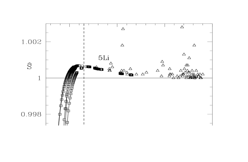
Figure 3: Dependence of the $5Li$ action (squares) and Wilson action (circles) on the instanton size. The triangles are data coming from Monte Carlo configurations generated with the Wilson action and cooled with 300 sweeps of $5Li$ cooling. The vertical dashed line indicates the location of the threshold $\rho_{0}=2.3$. The dotted curve is the value of the Wilson action for an instanton of size $\rho$ calculated at tree level to ${\cal O}(a^{2})$; it shows the deviation from scale invariance of the Wilson action.

In Fig. 3 we present a comparison between the size dependence of the $5Li$-action and Wilson action. Instantons of different sizes are extracted from various stages of Wilson cooling of 3 different starting configurations. The triangles are data from Monte Carlo instantons ($\beta=2.5,\ 12^{4}$ lattice) cooled with 300 sweeps of $5Li$ cooling. For the improved action the dependence on the size is close to a step-function, giving $8\pi^{2}$ to better than $0.1\%$ for $\rho>\rho_{0}$ and a steep descent (slightly configuration dependent) in the interval $(0.8-1.0)\rho_{0}$ [28]. As Fig. 3 shows clearly, there is a small energy barrier which prevents the decay of any instanton of size greater than $\rho_{0}$.

There are simpler actions with no ${\cal O}(a^{2})$ corrections, like the $\epsilon$ action described in section 2.1 with $\epsilon=0$, which have been shown to improve results on the susceptibility (see [36] for a QCD study using such an action). Our analysis indicates, however, that the ${\cal O}(a^{4})$ terms may be relatively important in the region of physical sizes and they may lead to shifts in the instanton size with cooling, as already observed by Brower et al [36]. These terms are also important in the threshold region, which tends to loose its step-function like behavior. The cooling dependence of the sizes will also make a scaling test more involved.

2.4 Finite Size Effects

Lattice instantons may differ from the continuum ansatz due also to the finite lattice volume, therefore the question of stability of instantons cannot be completely decoupled from finite size effects. The influence of finite size effects on the quantities we want to study comes mostly in two ways:

• They affect the stability of instantons under cooling. Since on a periodic hyper-torus self-dual $Q=\pm 1$ solutions do not exist [30], single instanton configurations will always collapse after a while during cooling. Of course if the lattice size is much larger than the instanton size there is a wide window of meta-stability for $Q=\pm 1$ which for all practical purposes would amount to stable instantons. This window can be enlarged by choosing at least one of the lattice sizes, say $N_{t}$, very large. The problem can be completely avoided by imposing twisted boundary conditions in one of the lattice directions. In this case our cooling algorithm guarantees stability of the cooled structures for any value of the topological charge and an indefinite number of cooling sweeps.

• There is a maximal instanton size $\rho_{\rm max}$, determined by the length of the lattice and by the boundary conditions, hence the large-size part of the size distribution will be cut off and distorted. Due to point (a) above, $\rho_{\rm max}$ will also depend on the total topological charge of the configuration. We have observed that for self-dual $Q=\pm 1$ configurations and for symmetric lattices with periodic boundary conditions (p.b.c.) $\rho_{\rm max}^{t}\approx N_{s}/5$ [32], for elongated lattices with p.b.c. $\rho_{\rm max}^{t}\approx N_{s}/4$ and for twisted boundary conditions (t.b.c.) $\rho_{\rm max}^{t}\approx 2N_{s}/5$. Moreover large instantons which “feel” the boundaries will typically be deformed by them. As a consequence for large instantons different size definitions can give quite different results. To obtain a size distribution free from this effect the typical physical instanton size has to be less than the maximal instanton size, $\rho_{\rm max}$, allowed by the lattice. Note however that for higher topological charge $\rho_{\rm max}$ can be larger and may not show such a strong dependence on boundary conditions, hence the previous estimate is quite conservative.

This provides a general window to retrieve the physical size distribution, which goes from the cooling threshold $\tilde{\rho}_{0}=2.3a$ to at most the maximal instanton size. The threshold is a feature of the algorithm and is essential in discarding dislocations; it is fixed by choosing $\beta$. As already said $\tilde{\rho}_{\rm max}$ is fixed by the lattice size, boundary conditions and topological charge of the configuration.

Point (a) is illustrated for $12^{4}$ and $12^{3}\times 36$ lattices on Fig. 4, where we also show for comparison the behavior of a $Q=2$ configuration. For $N_{s}=N_{t}=12$ p.b.c. the maximal instanton size (attained by over-improved cooling) is too close to our stability threshold $\rho_{0}=2.3$, in consequence any isolated instanton decays quite fast. We expect the region of meta-stability to be enlarged when $\tilde{\rho}_{\rm max}$ gets away from the threshold (see for instance the $12^{3}\times 36$ p.b.c. lattice). We stress that the instability only affects self-dual $Q=\pm 1$ configurations but not multi-instanton configurations and can be completely avoided by using twisted boundary conditions in at least one lattice direction. The effect on the susceptibility and size distribution measured on p.b.c. lattices will be less strong for large physical volumes where the contribution to the susceptibility of configurations with single instantons is smaller.

As an illustration of the uncertainties in assigning physical parameters to very large instantons we present in Table 2.4 data coming from the analysis of the maximal size instanton on a $12^{4}$ lattice with twisted boundary condition in time. Although this (completely stable) configuration has total charge 1 and action $8\pi^{2}$ the number of peaks in the energy density is 6 and in consequence a naive assignment of instantons to peaks will misleadingly interpret it as 6 different instantons, with quite large sizes and excentricity. On the other hand an analysis of the time profile reveals only one peak with much smaller size.

$(x,y,z,t){\vrule height=13.0pt,depth=6.0pt,width=0.0pt}$ $\rho_{c}{\vrule height=13.0pt,depth=6.0pt,width=0.0pt}$ $\rho_{p}{\vrule height=13.0pt,depth=6.0pt,width=0.0pt}$ $\epsilon_{c}{\vrule height=13.0pt,depth=6.0pt,width=0.0pt}$ $N{\vrule height=13.0pt,depth=6.0pt,width=0.0pt}$   $(3,4,2,2){\vrule height=13.0pt,depth=6.0pt,width=0.0pt}$ $7.90{\vrule height=13.0pt,depth=6.0pt,width=0.0pt}$ $7.22{\vrule height=13.0pt,depth=6.0pt,width=0.0pt}$ $0.66{\vrule height=13.0pt,depth=6.0pt,width=0.0pt}$ $-1.43{\vrule height=13.0pt,depth=6.0pt,width=0.0pt}$ $(4,6,2,2){\vrule height=13.0pt,depth=6.0pt,width=0.0pt}$ $7.61{\vrule height=13.0pt,depth=6.0pt,width=0.0pt}$ $7.09{\vrule height=13.0pt,depth=6.0pt,width=0.0pt}$ $0.58{\vrule height=13.0pt,depth=6.0pt,width=0.0pt}$ $-1.33{\vrule height=13.0pt,depth=6.0pt,width=0.0pt}$ $(1,1,3,2){\vrule height=13.0pt,depth=6.0pt,width=0.0pt}$ $7.38{\vrule height=13.0pt,depth=6.0pt,width=0.0pt}$ $6.96{\vrule height=13.0pt,depth=6.0pt,width=0.0pt}$ $0.58{\vrule height=13.0pt,depth=6.0pt,width=0.0pt}$ $-1.26{\vrule height=13.0pt,depth=6.0pt,width=0.0pt}$ $(6,7,3,2){\vrule height=13.0pt,depth=6.0pt,width=0.0pt}$ $7.31{\vrule height=13.0pt,depth=6.0pt,width=0.0pt}$ $7.00{\vrule height=13.0pt,depth=6.0pt,width=0.0pt}$ $0.45{\vrule height=13.0pt,depth=6.0pt,width=0.0pt}$ $-1.19{\vrule height=13.0pt,depth=6.0pt,width=0.0pt}$ $(10,4,5,2){\vrule height=13.0pt,depth=6.0pt,width=0.0pt}$ $10.06{\vrule height=13.0pt,depth=6.0pt,width=0.0pt}$ $7.52{\vrule height=13.0pt,depth=6.0pt,width=0.0pt}$ $2.21{\vrule height=13.0pt,depth=6.0pt,width=0.0pt}$ $-3.21{\vrule height=13.0pt,depth=6.0pt,width=0.0pt}$ $(10,10,5,2){\vrule height=13.0pt,depth=6.0pt,width=0.0pt}$ $7.93{\vrule height=13.0pt,depth=6.0pt,width=0.0pt}$ $7.23{\vrule height=13.0pt,depth=6.0pt,width=0.0pt}$ $0.66{\vrule height=13.0pt,depth=6.0pt,width=0.0pt}$ $-1.44{\vrule height=13.0pt,depth=6.0pt,width=0.0pt}$ Table 2.4: Assignment of parameters made by the fitting programs to the maximal size instanton ($\hat{S}=1.0000$, $Q=-1.0001$) on a $12^{4}$ t.b.c. lattice. $(x,y,z,t)$ represents the location of the 6 peaks in the action and charge densities. $N$ is the normalization appearing in the continuum ansatz, eq. (8), as given by the “center and nearest neighbors” fit (def.2) in section 2.2. Notice that all the peaks have the same time coordinate, hence only one peak will be detected in the integrated densities $s_{t}(t)$ and $q_{t}(t)$ eq. (13) giving a value $\rho_{\rm peak}^{t}=4.66$ (the time coordinate is selected by the twist).

3 SU(2) Topology by Improved Cooling

3.1 Simulation with Wilson Action

The first criterion for the physical relevance of all results is how they scale with the removal of the cut-off. We work in a region of $\beta$ where one expects to see scaling behavior, therefore all quantities of physical significance (susceptibility, charge distribution, size distribution, etc) should scale according to their dimension when approaching the continuum. As mentioned above, one may expect short-range topological excitations which are unphysical in the sense that they do not correspond to attributes of the continuum physics. These are therefore artifacts of the discretization and will show up as non-scaling, cut-off dependent structures in the results. Our algorithm has an inherent cut-off for such structure, the threshold $\rho_{0}\simeq 2.3$. Since the threshold is fixed in lattice units, it shrinks physically and it should not affect physical sizes if $a$ is small enough: the physical threshold ${\tilde{\rho}_{0}}\simeq 2.3a\rightarrow 0\ {\rm for}\ a\rightarrow 0$. This we shall test below when studying the scaling of various quantities. On the other hand, since Monte Carlo simulations with the Wilson action copiously produce short range fluctuations one can generally ask whether this shrinking cut-off at ${\tilde{\rho}_{0}}$ can indeed ensure the absence of unphysical fluctuations in cooled configurations when approaching the continuum.

Following an argument of Pugh and Teper [17] we write the contribution of small instantons of size $\rho_{0}$ to the partition function as ($N=2$ here)

$$\left[\rho_{0}(a)a\right]^{-4}\hbox{e}^{-S_{W}(\rho_{0})/g^{2}};\ \ a(\beta)\simeq\Lambda^{-1}\hbox{e}^{-{1\over{Ng^{2}\beta_{1}}}},\ \ \beta_{1}={{11N}\over{48\pi^{2}}}.$$

The contribution of instantons of a size $\rho$ such that $\hat{S}_{W}(\rho)<1/(2\pi^{2}N\beta_{1})=24/11N^{2}$ diverges for $\beta=4/g^{2}\rightarrow\infty$. We can calculate $\hat{S}_{W}(\rho)$ by cooling large instantons with the Wilson action and measuring the action and the size as the instantons shrink during cooling (see Fig. 3). This analysis leads to an UV threshold $1<\rho_{0}<2$. It is difficult to get a precise estimate since the dependence of $S_{W}$ on $\rho$ in this region is sensitive to details of the configuration. We can conclude, however, that our threshold $\rho_{0}$ of about 2.3 is fully satisfactory when dealing with configurations produced with the Wilson action: it ensures removal of the divergent contribution of lattice artifacts, without cutting too much from the physical sizes even at rather low $\beta$.

Likewise, the correction due to the finite lattice size should be estimated by changing the volume and/or boundary conditions and checking the sensitivity of the results to these changes. Quite generally, they will affect structures at the long-range edge of the size distribution. To estimate the importance of the finite lattice size effects we use both different physical volumes and boundary conditions.

We base our analysis on the following $SU(2)$ Monte Carlo simulations (heat–bath, Wilson action):

$N_{s}{\vrule height=13.0pt,depth=6.0pt,width=0.0pt}$ $N_{t}{\vrule height=13.0pt,depth=6.0pt,width=0.0pt}$ $\beta{\vrule height=13.0pt,depth=6.0pt,width=0.0pt}$ $a(\beta)\ ({\rm fm}){\vrule height=13.0pt,depth=6.0pt,width=0.0pt}$ $L\ ({\rm fm}){\vrule height=13.0pt,depth=6.0pt,width=0.0pt}$ ${\rm b.}\ {\rm cond.}{\vrule height=13.0pt,depth=6.0pt,width=0.0pt}$ $\#{\rm conf.}{\vrule height=13.0pt,depth=6.0pt,width=0.0pt}$ $\#{\rm sw.}\ {\rm betw.}\ {\rm conf.}{\vrule height=13.0pt,depth=6.0pt,width=0.0pt}$     ${\bf(1a)}{\vrule height=13.0pt,depth=6.0pt,width=0.0pt}$ $12{\vrule height=13.0pt,depth=6.0pt,width=0.0pt}$ $12{\vrule height=13.0pt,depth=6.0pt,width=0.0pt}$ $2.4{\vrule height=13.0pt,depth=6.0pt,width=0.0pt}$ $0.12{\vrule height=13.0pt,depth=6.0pt,width=0.0pt}$ $1.44{\vrule height=13.0pt,depth=6.0pt,width=0.0pt}$ ${\rm t.b.c.}{\vrule height=13.0pt,depth=6.0pt,width=0.0pt}$ $237{\vrule height=13.0pt,depth=6.0pt,width=0.0pt}$ $100{\vrule height=13.0pt,depth=6.0pt,width=0.0pt}$ ${\bf(1b)}{\vrule height=13.0pt,depth=6.0pt,width=0.0pt}$ $12{\vrule height=13.0pt,depth=6.0pt,width=0.0pt}$ $12{\vrule height=13.0pt,depth=6.0pt,width=0.0pt}$ $2.4{\vrule height=13.0pt,depth=6.0pt,width=0.0pt}$ $0.12{\vrule height=13.0pt,depth=6.0pt,width=0.0pt}$ $1.44{\vrule height=13.0pt,depth=6.0pt,width=0.0pt}$ ${\rm p.b.c.}{\vrule height=13.0pt,depth=6.0pt,width=0.0pt}$ $202{\vrule height=13.0pt,depth=6.0pt,width=0.0pt}$ $100{\vrule height=13.0pt,depth=6.0pt,width=0.0pt}$ ${\bf(1c)}{\vrule height=13.0pt,depth=6.0pt,width=0.0pt}$ $12{\vrule height=13.0pt,depth=6.0pt,width=0.0pt}$ $36{\vrule height=13.0pt,depth=6.0pt,width=0.0pt}$ $2.4{\vrule height=13.0pt,depth=6.0pt,width=0.0pt}$ $0.12{\vrule height=13.0pt,depth=6.0pt,width=0.0pt}$ $1.44{\vrule height=13.0pt,depth=6.0pt,width=0.0pt}$ ${\rm p.b.c.}{\vrule height=13.0pt,depth=6.0pt,width=0.0pt}$ $198{\vrule height=13.0pt,depth=6.0pt,width=0.0pt}$ $100{\vrule height=13.0pt,depth=6.0pt,width=0.0pt}$ ${\bf(2)}{\vrule height=13.0pt,depth=6.0pt,width=0.0pt}$ $12{\vrule height=13.0pt,depth=6.0pt,width=0.0pt}$ $12{\vrule height=13.0pt,depth=6.0pt,width=0.0pt}$ $2.5{\vrule height=13.0pt,depth=6.0pt,width=0.0pt}$ $0.085{\vrule height=13.0pt,depth=6.0pt,width=0.0pt}$ $1.02{\vrule height=13.0pt,depth=6.0pt,width=0.0pt}$ ${\rm t.b.c.}{\vrule height=13.0pt,depth=6.0pt,width=0.0pt}$ $160{\vrule height=13.0pt,depth=6.0pt,width=0.0pt}$ $250{\vrule height=13.0pt,depth=6.0pt,width=0.0pt}$ ${\bf(3)}{\vrule height=13.0pt,depth=6.0pt,width=0.0pt}$ $24{\vrule height=13.0pt,depth=6.0pt,width=0.0pt}$ $24{\vrule height=13.0pt,depth=6.0pt,width=0.0pt}$ $2.6{\vrule height=13.0pt,depth=6.0pt,width=0.0pt}$ $0.06{\vrule height=13.0pt,depth=6.0pt,width=0.0pt}$ $1.44{\vrule height=13.0pt,depth=6.0pt,width=0.0pt}$ ${\rm t.b.c.}{\vrule height=13.0pt,depth=6.0pt,width=0.0pt}$ $84{\vrule height=13.0pt,depth=6.0pt,width=0.0pt}$ $200{\vrule height=13.0pt,depth=6.0pt,width=0.0pt}$ Table 3.1: Ensembles of gauge field configurations analyzed; t.b.c lattices have $k=(1,1,1)$ twist in the time direction and periodic boundary conditions in space; p.b.c. lattices have periodic boundary conditions in all directions.

where we have estimated $a(\beta)$ using the 1-loop phenomenological formula (derived from data in [37])

$$a(\beta)=400\exp{\biggl{\{}-\frac{\beta\ln 2}{0.205}\biggr{\}}}\ {\rm fm}.$$ (19)

Here all data are taken after 20000 sweeps for thermalization. Part of these data have been presented at the Lattice’95 [28] and Lattice’96 [29] conferences.

As a rule, during cooling we performed measurements after 5, 20, 50, 150 and 300 cooling sweeps for lattices (1) and (3), and every 20 sweeps for lattice (2) (up to 300).

We typically calculate the $5Li$ charge and electric and magnetic action 4-dimensional densities and thereby the total topological charge and action of the configurations.

3.2 Topological Susceptibility and Charge Distribution

Since the topological charge $Q(5Li)$ stabilizes very fast to an integer within less than $1\%$, we expect deviations from the physical values in the susceptibility to be only due to threshold or to finite size effects. Our results are presented in Fig. 5 and Table 3.2a. The susceptibility (from $Q(5Li)$) settles early in the cooling. It scales very well with the cut-off (compare the (1) and (3) data) and shows little dependence on the volume (compare lattices (1a-b) and (3) with (1c) and with (2)). Data coming from the smaller physical volume seem to be higher by about 5$\%$, although they are compatible within errors with the other two determinations. The effect can be due to our particular estimation of the physical scale eq. (19) or it can be a volume effect (that the lattice size for these data is too small is evident in the size distribution – see next section). The small decrease in the susceptibility during cooling showing up in the data from lattices (1) ($\beta=2.4$) appears to be mostly a threshold effect. Our cutoff on small sizes ($\tilde{\rho}_{0}=2.3a$) will induce a systematic underestimate in the measurement of the susceptibility since some physical instantons might be eliminated, but this error goes down with increasing $\beta$ and can be easily estimated using the size distribution. As we will see in section 3.3 we obtain size distributions which scale nicely. Based on the fit to these distributions this underestimate should be about $3\%$ for $a=0.12$fm and less than $1\%$ for $a=0.06$fm. This is compatible with the difference between short and long cooling values (see Table 3.2a.) and does not change significantly the overall picture. Assuming the Witten – Veneziano formula to hold, our result $\chi^{1/4}=200(15)$MeV agrees excellently with the phenomenological expectation.

Recent results for $\chi^{1/4}$ in SU(2) [25] are about $20\%$ higher (for $\chi$ itself they are about a factor of two larger). We believe the discrepancy might be caused by the presence of some dislocations in the data of [25]. It would be very interesting to have data for the size distribution extracted using inverse blocking. A scaling check on such distribution will provide an unambiguous way of deciding whether dislocations are still present, since their contribution to the size distribution does not scale.

Further confidence in the correctness of our results for the topological susceptibility has been provided by R. Narayanan and P. Vranas [14]. They have used the overlap formalism [13] to measure the topological susceptibility on a $12^{4}$ lattice at $\beta=2.4$ with periodic boundary conditions (our (1b) lattice). Their results for the topological susceptibility as well as for the charge distribution are in perfect agreement, within errors, with ours.

Note that the early stabilization of the susceptibility with cooling is not only due to the efficiency of the improved algorithm in removing dislocations, but also to the fact that we use the improved charge operator $Q(5Li)$. To illustrate this we present in Table 3.2b the values of the topological susceptibility, for lattices (1a) and (2) in Table 3.1, extracted from the measurement of $Q(W)$ over the same set of $5Li$ cooled configurations. $(1{\rm a)}{\vrule height=13.0pt,depth=6.0pt,width=0.0pt}$ $(1{\rm b)}{\vrule height=13.0pt,depth=6.0pt,width=0.0pt}$ $(1{\rm c)}{\vrule height=13.0pt,depth=6.0pt,width=0.0pt}$ $(3){\vrule height=13.0pt,depth=6.0pt,width=0.0pt}$ $(2){\vrule height=13.0pt,depth=6.0pt,width=0.0pt}$   ${\rm sw}{\vrule height=13.0pt,depth=6.0pt,width=0.0pt}$ $5Li{\vrule height=13.0pt,depth=6.0pt,width=0.0pt}$ $5Li{\vrule height=13.0pt,depth=6.0pt,width=0.0pt}$ $5Li{\vrule height=13.0pt,depth=6.0pt,width=0.0pt}$ $5Li{\vrule height=13.0pt,depth=6.0pt,width=0.0pt}$ ${\rm sw}{\vrule height=13.0pt,depth=6.0pt,width=0.0pt}$ $5Li{\vrule height=13.0pt,depth=6.0pt,width=0.0pt}$     $0{\vrule height=13.0pt,depth=6.0pt,width=0.0pt}$ $161(5){\vrule height=13.0pt,depth=6.0pt,width=0.0pt}$ $0{\vrule height=13.0pt,depth=6.0pt,width=0.0pt}$ $219(8){\vrule height=13.0pt,depth=6.0pt,width=0.0pt}$ $5{\vrule height=13.0pt,depth=6.0pt,width=0.0pt}$ $199(3){\vrule height=13.0pt,depth=6.0pt,width=0.0pt}$ $200(5){\vrule height=13.0pt,depth=6.0pt,width=0.0pt}$ $201(5){\vrule height=13.0pt,depth=6.0pt,width=0.0pt}$ $205(16){\vrule height=13.0pt,depth=6.0pt,width=0.0pt}$ $20{\vrule height=13.0pt,depth=6.0pt,width=0.0pt}$ $200(3){\vrule height=13.0pt,depth=6.0pt,width=0.0pt}$ $200(6){\vrule height=13.0pt,depth=6.0pt,width=0.0pt}$ $199(5){\vrule height=13.0pt,depth=6.0pt,width=0.0pt}$ $199(15){\vrule height=13.0pt,depth=6.0pt,width=0.0pt}$ $20{\vrule height=13.0pt,depth=6.0pt,width=0.0pt}$ $212(7){\vrule height=13.0pt,depth=6.0pt,width=0.0pt}$ $50{\vrule height=13.0pt,depth=6.0pt,width=0.0pt}$ $198(3){\vrule height=13.0pt,depth=6.0pt,width=0.0pt}$ $198(6){\vrule height=13.0pt,depth=6.0pt,width=0.0pt}$ $195(5){\vrule height=13.0pt,depth=6.0pt,width=0.0pt}$ $197(15){\vrule height=13.0pt,depth=6.0pt,width=0.0pt}$ $60{\vrule height=13.0pt,depth=6.0pt,width=0.0pt}$ $212(7){\vrule height=13.0pt,depth=6.0pt,width=0.0pt}$ $150{\vrule height=13.0pt,depth=6.0pt,width=0.0pt}$ $196(4){\vrule height=13.0pt,depth=6.0pt,width=0.0pt}$ $195(6){\vrule height=13.0pt,depth=6.0pt,width=0.0pt}$ $192(6){\vrule height=13.0pt,depth=6.0pt,width=0.0pt}$ $197(15){\vrule height=13.0pt,depth=6.0pt,width=0.0pt}$ $140{\vrule height=13.0pt,depth=6.0pt,width=0.0pt}$ $212(7){\vrule height=13.0pt,depth=6.0pt,width=0.0pt}$ $300{\vrule height=13.0pt,depth=6.0pt,width=0.0pt}$ $195(4){\vrule height=13.0pt,depth=6.0pt,width=0.0pt}$ $193(6){\vrule height=13.0pt,depth=6.0pt,width=0.0pt}$ $189(6){\vrule height=13.0pt,depth=6.0pt,width=0.0pt}$ $194(14){\vrule height=13.0pt,depth=6.0pt,width=0.0pt}$ $300{\vrule height=13.0pt,depth=6.0pt,width=0.0pt}$ $211(7){\vrule height=13.0pt,depth=6.0pt,width=0.0pt}$ Table 3.2a: ${}^{4}\sqrt{\chi}$ (MeV) computed from the improved charge operator $Q(5Li)$, vs number of cooling sweeps. Errors have been estimated using the jackknife method.

The susceptibility stabilizes much earlier with cooling if the improved operator is used. Indeed even when no cooling at all is performed, the deviation from the asymptotic value is at most $20\%$ for $Q(5Li)$ while it is twice as much for the naive charge operator (after 5 sweeps $Q(5Li)$ is already asymptotic while $Q(W)$ is still $10\%$ off). The results obtained with $Q(5Li)$ after only a few cooling sweeps deviate by no more than $0.5\%$ from what is obtained by approximating the charge by the closest integer. Even without cooling the deviation is only about $1-2\%$. This rounding procedure also works for $Q(W)$, but only after a long cooling: approximating the charge by the closest integer after 300 sweeps we obtain ${}^{4}\sqrt{\chi}=194(4)$, 212(7) (MeV) for (1a) and (2) respectively, in perfect agreement with the results from $Q(5Li)$. The importance of improving the topological charge operator for non-smooth configurations has been recently stressed in [22].

$(1{\rm a)}{\vrule height=13.0pt,depth=6.0pt,width=0.0pt}$ $(2){\vrule height=13.0pt,depth=6.0pt,width=0.0pt}$   ${\rm sw}{\vrule height=13.0pt,depth=6.0pt,width=0.0pt}$ ${\rm Wilson}{\vrule height=13.0pt,depth=6.0pt,width=0.0pt}$ ${\rm sw}{\vrule height=13.0pt,depth=6.0pt,width=0.0pt}$ ${\rm Wilson}{\vrule height=13.0pt,depth=6.0pt,width=0.0pt}$     $0{\vrule height=13.0pt,depth=6.0pt,width=0.0pt}$ $123(3){\vrule height=13.0pt,depth=6.0pt,width=0.0pt}$ $0{\vrule height=13.0pt,depth=6.0pt,width=0.0pt}$ $167(6){\vrule height=13.0pt,depth=6.0pt,width=0.0pt}$ $5{\vrule height=13.0pt,depth=6.0pt,width=0.0pt}$ $179(3){\vrule height=13.0pt,depth=6.0pt,width=0.0pt}$ $20{\vrule height=13.0pt,depth=6.0pt,width=0.0pt}$ $186(3){\vrule height=13.0pt,depth=6.0pt,width=0.0pt}$ $20{\vrule height=13.0pt,depth=6.0pt,width=0.0pt}$ $201(6){\vrule height=13.0pt,depth=6.0pt,width=0.0pt}$ $50{\vrule height=13.0pt,depth=6.0pt,width=0.0pt}$ $188(3){\vrule height=13.0pt,depth=6.0pt,width=0.0pt}$ $60{\vrule height=13.0pt,depth=6.0pt,width=0.0pt}$ $204(7){\vrule height=13.0pt,depth=6.0pt,width=0.0pt}$ $150{\vrule height=13.0pt,depth=6.0pt,width=0.0pt}$ $188(4){\vrule height=13.0pt,depth=6.0pt,width=0.0pt}$ $140{\vrule height=13.0pt,depth=6.0pt,width=0.0pt}$ $204(6){\vrule height=13.0pt,depth=6.0pt,width=0.0pt}$ $300{\vrule height=13.0pt,depth=6.0pt,width=0.0pt}$ $187(4){\vrule height=13.0pt,depth=6.0pt,width=0.0pt}$ $300{\vrule height=13.0pt,depth=6.0pt,width=0.0pt}$ $204(6){\vrule height=13.0pt,depth=6.0pt,width=0.0pt}$ Table 3.2b: ${}^{4}\sqrt{\chi}$ (MeV) computed from the naive charge operator $Q(W)$ vs number of cooling sweeps.

The topological charge distribution is presented in Fig. 6 for various boundary conditions and numbers of cooling sweeps. The differences induced by the former are related mostly to the instability of self-dual charge $\pm 1$ configurations for periodic boundary conditions (the p.b.c. data show typically more configurations at $Q=0$ and fewer at $Q=\pm 1$ than the t.b.c. data, but the statistics is not sufficient for a significant signal). The disappearance of some narrow peaks (beyond pair annihilation) when going from 20 to 300 cooling sweeps does not lead to significant changes in the distribution. The shape of the charge distribution agrees well with a gaussian of width given by the susceptibility. These data are also nicely corroborated by those from [14].

3.3 Instanton Shape and Size Distribution

For a systematic analysis of the local structure we developed a number of programs to automatically recognize and evaluate the local features. We think it useful to give some technical details about the procedure, to permit an overview of the various constraints and uncertainties.

Essentially these programs proceed by finding first the peaks in the action and in the topological charge density. The identification of the peaks proceeds along the following three steps:

• Look for peaks in the electric and magnetic parts of the action density, $E^{2}(x)$ and $B^{2}(x)$. Assign a peak to every lattice point whose density is maximal with respect to its nearest neighbors. We also assign a normalization $\pm 1$ to each peak depending on whether its topological charge is positive or negative.

• Apply a cut that removes from the set of peaks those which are so flat that $\rho_{{\rm peak}}(S)$ is larger than $N_{s}$. Typically small fluctuations, not associated to instantons, or remnants of I-A annihilation will give rise to very low peaks in the energy density, which misleadingly translate via the $\rho_{\rm peak}$ formula eq. (14) into very large sizes. With this cut we suppress part of these effects.

• Apply a cut from self-duality by comparing the locations of peaks in $E^{2}(x)$ and $B^{2}(x)$ (with equal normalization). Only peaks for which the distance between locations is less than or equal to $2a$ are kept.

After performing these cuts we have observed that there is an abundance of close peaks separated from each other no more than 1 lattice spacing along each direction. This behavior has been also pointed out in [21]. We have adopted the attitude of identifying such peaks as being only one. We believe that the effect is mostly due to locating peaks by looking only at nearest neighbors and not at points separated along the diagonal (slightly excentric instantons located diagonally between the lattice points may lead to such a signal). The effect of this last cut reduces the number of peaks by about $8\%$ independently of the number of cooling sweeps. It is important to point out that the cut is applied in lattice units so if there is indeed a physical effect associated to close peaks it should be possible to detect it anyway by reducing the lattice spacing. In section 3.4.2 we will discuss further this effect by comparing results from lattices with $a=0.12$ fm and $a=0.06$ fm.

The typical level of accuracy achieved by these programs turned out to be above $90\%$, the failures being mostly related to structures affected by threshold or by finite size effects (e.g., wrong normalization, misinterpretation of a wide, deformed instanton as a multiple peak structure, etc). While global quantities like total charge or topological susceptibility are not affected by such uncertainties, the latter will be reflected in systematic errors concerning, e.g., the small and large size edges of the size distributions. The errors we quote in this paper are statistical only. But we now proceed to estimate the systematic errors.

3.3.1 Determination of Instanton Shape and Size

Both finite size effects and instanton - (anti-)instanton interaction may deform the spherically symmetric, continuum ansatz and we did not want to bias a priori the information about instanton shape by assuming spherical symmetry. We decided therefore to evaluate simultaneously several of the size definitions in section 2.2. A comparison between them and more specifically a measurement of the excentricity (see eq. (10)) provides a good estimate of the departure from the continuum ansatz. Our analysis proceeds along two directions:

• Extracting “on line” sizes corresponding to definitions 1, 2, 5 in section 2.2 (i.e. $\rho_{\rm peak}$, $\rho_{c}$ and $\rho_{d}(R)$ for $R=\rho_{\rm peak}$ and $R=\rho_{\rm peak}/\sqrt{2}$). We also extract the excentricity $\epsilon_{c}$ using (def.2) in section 2.2.

• Performing by MINUIT global fits of the $5Li$ charge and action densities using eq. (8). In most cases this ansatz fits rather well the $5Li$-densities (charge and action) of isolated instantons already after a few cooling sweeps. The simple superposition extension of this ansatz can also handle overlapping structures in multi-peak fits over clusters.

We tried to assess the uncertainty of the analysis self-consistently by comparing all the size definitions.

The global fits (b) start with initial information about the location and size of the peaks provided by (a). Clusters are first identified, by considering as neighbors peaks at a distance less than their average radius. For this we use the size estimate from (a), or a fraction thereof if we want to limit the maximal cluster size (MINUIT would not cope with more than 5 peaks at a time). Once identified, the clusters are fitted separately with a superposition ansatz. The MINUIT fit uses 8 or 9 parameters per peak (in the latter case the normalization $N$ in eq. (8) is taken as a real number and permitted to vary). The fitting procedure tends to fail in the cases where also the peak assignment is not well defined (see the discussion in sect. 2.4). For the description of the topological structure uncovered in this way we shall use the geometric average size eq. (9) and the “excentricity” eq. (10). Since the global fits are rather expensive we performed them only on subsets of 10 configurations for the (1a) and (1b) lattices and 5 configurations on (1c) (for the $24^{4}$ lattices we could not perform global fits on our workstations), therefore the data for $\rho_{f}$ and $\epsilon_{f}$ ((def.3), section 2.2) have large statistical errors.

A comparison between the fit analysis, $\rho_{{\rm peak}}$, (def.1) and $\rho_{c}$ (def.2) is given in Table 3.3.1a. The differences in the results for size and the excentricities are presented as the root mean squares $\delta\rho/\rho|_{\rm rms}$ and $\epsilon_{f}|_{\rm rms}$, with $\delta\rho/\rho=2(\rho_{{\rm peak}}-\rho)/(\rho_{{\rm peak}}+\rho)$. Here $\rho=\rho_{c}$ or $\rho=\rho_{f}$ as obtained from the following fits: “f4” (free norm cluster fit with up to 4 peaks in a cluster), “fn” (cluster fit with up to 4 peaks in a cluster with the norm $N=\pm 1$ as assigned by (a)) and “fs” (single peak fit with the norm $N$ taken as free parameter). The figures in brackets correspond to discarding peaks for which one or more of the sizes are larger than the lattice size – these cases typically prove to be I-A pairs in the course of annihilation or simply failures of the fit program in the presence of very distorted structures. They affect $5-10\%$ of the peaks.

As can be seen, the fitted radius averaged over directions agrees quite well with $\rho_{{\rm peak}}$ (def.1). From the data in Table 3.3.1a we estimate a total error of less than $10\%$ for long cooling: we reproduce this (informal) estimation $\sigma(\rho)$ in Table 3.3.1b. Both $\sigma(\rho)$ and $\epsilon_{f}|_{\rm rms}$ decrease with the number of cooling sweeps, which is understandable as an effect of smoothing and of the disappearance of I-A pairs.

In Fig. 7 we compare the size distributions obtained from the $\rho_{peak}$ and $\rho_{c}$ data. We also show here the “excentricity” distribution $\epsilon_{c}$. As is evident in the cross-correlation between size and excentricity on Fig. 7, larger instantons depart more from the spherical shape. Also, the average excentricity decreases with cooling. The excentricity can have at least four origins:

• sensitivity of the fit procedure to details of the configuration not considered in the ansatz, e.g., the presence of nearby instantons;

• interaction among (anti-)instantons, which is not taken care of by the ansatz;

• physical fluctuations (e.g., higher momentum states) in the ensemble of instantons produced in the Monte Carlo simulation at physical sizes;

• distortion of the true lattice instantons at large sizes due to finite volume effects.

Both the first and second effect are stronger if the instantons have a large overlap, therefore they should decrease with cooling as a result of the dilution of the ensemble due to pair annihilation. For the same reason they also could affect large instantons more than small ones. The smoothing out of physical fluctuations during cooling will tend to decrease the average excentricity for instantons in the range of sizes not affected by finite volume effects, since there the exact solution is spherically symmetric; this does not necessarily hold for large instantons, which may be very deformed asymptotically. Fig. 7 shows that excentric instantons are rare. We have explicitly verified that the 4 axes $\rho_{\mu}$ of our ellipsoidal fits are strongly correlated. Departure from spherical symmetry is moderate, and well accounted for by our ellipsoidal ansatz, eq.(8).

In Fig. 8 we compare sizes obtained from definitions 1 and 5 (see section 2.2): $\rho_{\rm peak}(S)$, $\rho_{\rm peak}(Q)$ or $\rho_{d}(R)$. All should agree if the continuum ansatz is correct. As we can see, the differences are typically well within the uncertainty estimated on the basis of the fits, and mostly affect large instantons of size above $N_{s}/2$. The effects related to large instantons are clearly reflected in Fig. 9 where we compare size distributions after 300 cooling sweeps extracted from $\rho_{{\rm peak}}(Q)$ (def.1) and $\rho_{\rm f}^{t}$ (def.4) for lattice (2) ($12^{4}$ at $\beta=2.5$, physical size approximately 1fm). The $\rho_{\rm f}^{t}$ distribution has a strong large size cutoff around $N_{s}/2$ while the $\rho_{{\rm peak}}(Q)$ one is quite biased towards large sizes. In addition the number of peaks in the energy density is larger by as much as $40\%$ than the one extracted from spatially integrated densities (it decreases from 98 to 61 after integration for 70 configurations analyzed).

A further measurement of the good agreement between different size definitions is provided by the value of the normalization entering in the density formula eq. (8) (see also eq. (15)). In Fig. 10 we present the histogram for the distribution of normalizations obtained from the “center and nearest neighbors” analysis (def.2). It is nicely centered about $\pm 1$ with a dispersion that decreases with the number of cooling sweeps due to effects analogous to the ones quoted above in relation with the excentricity.

$\hskip 14.22636pt(1{\rm a})\ \ \ {\rm t.b.c}{\vrule height=13.0pt,depth=6.0pt,width=0.0pt}$ $\hskip 14.22636pt(1{\rm b})\ \ \ {\rm p.b.c.}{\vrule height=13.0pt,depth=6.0pt,width=0.0pt}$ $\hskip 14.22636pt(1{\rm c})\ \ \ {\rm p.b.c.\ elongated}{\vrule height=13.0pt,depth=6.0pt,width=0.0pt}$   ${\rm sw}\!{\vrule height=13.0pt,depth=6.0pt,width=0.0pt}$ ${\rm fit}{\vrule height=13.0pt,depth=6.0pt,width=0.0pt}$ $\#{\rm peaks}\hskip 5.69054pt\frac{\delta\rho}{\rho}|_{\rm rms}\hskip 8.5359pt\ \epsilon_{f}|_{\rm rms}{\vrule height=13.0pt,depth=6.0pt,width=0.0pt}$ $\#{\rm peaks}\hskip 14.22636pt\frac{\delta\rho}{\rho}|_{\rm rms}\hskip 8.5359pt\ \epsilon_{f}|_{\rm rms}{\vrule height=13.0pt,depth=6.0pt,width=0.0pt}$ $\#{\rm peaks}\hskip 14.22636pt\frac{\delta\rho}{\rho}|_{\rm rms}\hskip 8.5359pt\ \epsilon_{f}|_{\rm rms}{\vrule height=13.0pt,depth=6.0pt,width=0.0pt}$     $c{\vrule height=13.0pt,depth=6.0pt,width=0.0pt}$ $\ 98\ \ \ \ \ \ \ 0.125\hskip 17.07182pt0.427{\vrule height=13.0pt,depth=6.0pt,width=0.0pt}$ $\ 103\ \ \ \ \ \ \ 0.117\hskip 17.07182pt0.333{\vrule height=13.0pt,depth=6.0pt,width=0.0pt}$ $\ 172\ \ \ \ \ \ \ 0.079\hskip 17.07182pt0.552{\vrule height=13.0pt,depth=6.0pt,width=0.0pt}$ $(96)\ \ \ \ (0.115)\hskip 8.53581pt(0.318){\vrule height=13.0pt,depth=6.0pt,width=0.0pt}$ $(101)\ \ \ \ (0.109)\hskip 8.53581pt(0.290){\vrule height=13.0pt,depth=6.0pt,width=0.0pt}$ $(171)\ \ \ \ (0.076)\hskip 8.53581pt(0.552){\vrule height=13.0pt,depth=6.0pt,width=0.0pt}$ $fn{\vrule height=13.0pt,depth=6.0pt,width=0.0pt}$ $\ 98\ \ \ \ \ \ \ 0.125\hskip 17.07182pt1.427{\vrule height=13.0pt,depth=6.0pt,width=0.0pt}$ $\ 103\ \ \ \ \ \ \ 0.203\hskip 17.07182pt1.563{\vrule height=13.0pt,depth=6.0pt,width=0.0pt}$ $\ 172\ \ \ \ \ \ \ 0.099\hskip 17.07182pt0.622{\vrule height=13.0pt,depth=6.0pt,width=0.0pt}$ $20\!{\vrule height=13.0pt,depth=6.0pt,width=0.0pt}$ $(96)\ \ \ \ (0.123)\hskip 8.53581pt(0.386){\vrule height=13.0pt,depth=6.0pt,width=0.0pt}$ $\ (94)\ \ \ \ \ (0.205)\hskip 8.53581pt(0.375){\vrule height=13.0pt,depth=6.0pt,width=0.0pt}$ $(168)\ \ \ \ (0.093)\hskip 8.53581pt(0.414){\vrule height=13.0pt,depth=6.0pt,width=0.0pt}$ $f4{\vrule height=13.0pt,depth=6.0pt,width=0.0pt}$ $\ 98\ \ \ \ \ \ \ 0.176\hskip 17.07164pt0.536{\vrule height=13.0pt,depth=6.0pt,width=0.0pt}$ $\ 103\ \ \ \ \ \ \ 0.191\hskip 17.07182pt0.962{\vrule height=13.0pt,depth=6.0pt,width=0.0pt}$ $\ 172\ \ \ \ \ \ \ 0.184\hskip 17.07182pt0.808{\vrule height=13.0pt,depth=6.0pt,width=0.0pt}$ $(95)\ \ \ \ (0.170)\hskip 8.53581pt(0.326){\vrule height=13.0pt,depth=6.0pt,width=0.0pt}$ $(101)\ \ \ \ (0.158)\hskip 8.53581pt(0.308){\vrule height=13.0pt,depth=6.0pt,width=0.0pt}$ $(165)\ \ \ \ (0.176)\hskip 8.53581pt(0.404){\vrule height=13.0pt,depth=6.0pt,width=0.0pt}$ $fs{\vrule height=13.0pt,depth=6.0pt,width=0.0pt}$ $\ 98\ \ \ \ \ \ \ 0.140\hskip 17.07182pt0.527{\vrule height=13.0pt,depth=6.0pt,width=0.0pt}$ $\ 103\ \ \ \ \ \ \ 0.157\hskip 17.07182pt0.352{\vrule height=13.0pt,depth=6.0pt,width=0.0pt}$ $\ 172\ \ \ \ \ \ \ 0.144\hskip 17.07182pt0.384{\vrule height=13.0pt,depth=6.0pt,width=0.0pt}$ $(97)\ \ \ \ (0.136)\hskip 8.53581pt(0.293){\vrule height=13.0pt,depth=6.0pt,width=0.0pt}$ $(101)\ \ \ \ (0.158)\hskip 8.53581pt(0.308){\vrule height=13.0pt,depth=6.0pt,width=0.0pt}$ $(171)\ \ \ \ (0.143)\hskip 8.53581pt(0.375){\vrule height=13.0pt,depth=6.0pt,width=0.0pt}$     $c{\vrule height=13.0pt,depth=6.0pt,width=0.0pt}$ $\ 17\ \ \ \ \ \ \ 0.033\hskip 17.07182pt0.211{\vrule height=13.0pt,depth=6.0pt,width=0.0pt}$ $\ \ 15\ \ \ \ \ \ \ 0.246\hskip 17.07182pt0.248{\vrule height=13.0pt,depth=6.0pt,width=0.0pt}$ $\ \ 28\ \ \ \ \ \ \ 0.065\hskip 17.07182pt0.221{\vrule height=13.0pt,depth=6.0pt,width=0.0pt}$ $(17){\vrule height=13.0pt,depth=6.0pt,width=0.0pt}$ $\ (13)\ \ \ \ (0.084)\hskip 9.95863pt(0.115){\vrule height=13.0pt,depth=6.0pt,width=0.0pt}$ $\ (28){\vrule height=13.0pt,depth=6.0pt,width=0.0pt}$ $fn{\vrule height=13.0pt,depth=6.0pt,width=0.0pt}$ $\ 17\ \ \ \ \ \ \ 0.095\hskip 17.07182pt0.295{\vrule height=13.0pt,depth=6.0pt,width=0.0pt}$ $\ \ 15\ \ \ \ \ \ \ 0.222\hskip 17.07182pt0.253{\vrule height=13.0pt,depth=6.0pt,width=0.0pt}$ $\ \ 28\ \ \ \ \ \ \ 0.100\hskip 17.07182pt0.409{\vrule height=13.0pt,depth=6.0pt,width=0.0pt}$ $300\!{\vrule height=13.0pt,depth=6.0pt,width=0.0pt}$ $(17){\vrule height=13.0pt,depth=6.0pt,width=0.0pt}$ $\ (13)\ \ \ \ (0.083)\hskip 9.95863pt(0.153){\vrule height=13.0pt,depth=6.0pt,width=0.0pt}$ $\ (27)\ \ \ \ \ (0.060)\hskip 7.11317pt(0.211){\vrule height=13.0pt,depth=6.0pt,width=0.0pt}$ $f4{\vrule height=13.0pt,depth=6.0pt,width=0.0pt}$ $\ 17\ \ \ \ \ \ \ 0.101\hskip 17.07164pt0.275{\vrule height=13.0pt,depth=6.0pt,width=0.0pt}$ $\ \ 15\ \ \ \ \ \ \ 0.179\hskip 17.07182pt0.274{\vrule height=13.0pt,depth=6.0pt,width=0.0pt}$ $\ \ 28\ \ \ \ \ \ \ 0.064\hskip 17.07182pt0.246{\vrule height=13.0pt,depth=6.0pt,width=0.0pt}$ $(17){\vrule height=13.0pt,depth=6.0pt,width=0.0pt}$ $\ (13)\ \ \ \ (0.021)\hskip 9.95863pt(0.127){\vrule height=13.0pt,depth=6.0pt,width=0.0pt}$ $\ (28){\vrule height=13.0pt,depth=6.0pt,width=0.0pt}$ $fs{\vrule height=13.0pt,depth=6.0pt,width=0.0pt}$ $\ 17\ \ \ \ \ \ \ 0.101\hskip 17.07182pt0.272{\vrule height=13.0pt,depth=6.0pt,width=0.0pt}$ $\ \ 15\ \ \ \ \ \ \ 0.238\hskip 17.07182pt0.391{\vrule height=13.0pt,depth=6.0pt,width=0.0pt}$ $\ \ 28\ \ \ \ \ \ \ 0.092\hskip 17.07182pt0.274{\vrule height=13.0pt,depth=6.0pt,width=0.0pt}$ $(17){\vrule height=13.0pt,depth=6.0pt,width=0.0pt}$ $\ (13)\ \ \ \ (0.021)\hskip 9.95863pt(0.121){\vrule height=13.0pt,depth=6.0pt,width=0.0pt}$ $\ (28){\vrule height=13.0pt,depth=6.0pt,width=0.0pt}$   Table 3.3.1a: Comparison of fit sizes and excentricities

$(1{\rm a}){\vrule height=13.0pt,depth=6.0pt,width=0.0pt}$ $(1{\rm b}){\vrule height=13.0pt,depth=6.0pt,width=0.0pt}$ $(1{\rm c}){\vrule height=13.0pt,depth=6.0pt,width=0.0pt}$ ${\rm sw}{\vrule height=13.0pt,depth=6.0pt,width=0.0pt}$ $\sigma(\rho){\vrule height=13.0pt,depth=6.0pt,width=0.0pt}$ $\sigma(\rho){\vrule height=13.0pt,depth=6.0pt,width=0.0pt}$ $\sigma(\rho){\vrule height=13.0pt,depth=6.0pt,width=0.0pt}$   $20{\vrule height=13.0pt,depth=6.0pt,width=0.0pt}$ $0.14\ (0.12){\vrule height=13.0pt,depth=6.0pt,width=0.0pt}$ $0.16\ (0.15){\vrule height=13.0pt,depth=6.0pt,width=0.0pt}$ $0.14\ (0.14){\vrule height=13.0pt,depth=6.0pt,width=0.0pt}$ $300{\vrule height=13.0pt,depth=6.0pt,width=0.0pt}$ $0.06\ (0.06){\vrule height=13.0pt,depth=6.0pt,width=0.0pt}$ $0.20\ (0.05){\vrule height=13.0pt,depth=6.0pt,width=0.0pt}$ $0.08\ (0.06){\vrule height=13.0pt,depth=6.0pt,width=0.0pt}$ Table 3.3.1b: Informal estimation of systematic errors

A general conclusion from the analysis described above is the good agreement, up to at most 10$\%$ discrepancy, of all the size definitions. Discrepancies appear due mostly to finite size effects and I-A pairs in the late stages of annihilation, which typically reflect in a departure from spherical symmetry and a wrong assignment of peaks. Based on these observations, we decided to quote in the following results for $\rho_{{\rm peak}}$ (def.1, eq. (14)) only. (In [28] the instanton sizes for lattice (2) were extracted from the t-profiles – see eq. (16)). Systematic errors in the determination of the size are estimated to be at most $10\%$.

For the lattice (3), we used lattice coordinates in eq. (14) to define the instanton center and no continuous interpolation of $O_{\mu}(x_{\mu})$ in ${x}_{\mu}$ was attempted. This may lead to an overestimation of the instanton size by up to $1/\rho^{2}$ which for the smallest stable instantons allowed by our algorithm, $\rho=2.3$, amounts to at most about 15$\%$, while for the typical size instanton it is below $2\%$.

3.3.2 Instanton Size Distribution

The results for the size distributions are presented in Fig. 11. We only compare the size distributions for lattices (1) and (3) since for lattice (2) the large-size edge of the distribution is strongly affected by finite size effects (see discussion in section 3.3.1 and Fig. 9). $P(\tilde{\rho})$ counts the number of instantons at distance $\tilde{\rho}$ normalized in such a way that the integral over $\tilde{\rho}$ is equal to 1.

The primary criterion for the physical significance of these distributions is how they scale in approaching the continuum limit. As we see from Fig. 11 the threshold (indicated by the vertical dashed line) is gradually removed with decreasing $a$ and the distributions scale nicely above it. The data at $\beta=2.6$ show that most of the physically relevant structure is in a well defined region above the threshold, where the latter has no influence. Comparison of the (1) and (3) data shows that at $\beta=2.4$ the bulk of the size distribution already begins to get out of the threshold region. The slight decay of the susceptibility with cooling observed in Table 3.2a and Fig. 5 for $\beta=2.4$ can be completely understood as due to the disappearance of a few, small but still physically relevant instantons close to the threshold (compare in Fig. 11 the distribution of instantons close to the threshold between 20 and 300 cooling sweeps). This good scaling of the distributions when changing the lattice cut off by a factor 2 gives evidence for their physical relevance. The stability under cooling of the distributions is also a check of the physical relevance of the results and the success of our algorithm in preserving the structure of the original configurations.

In Table 3.3.2 we give the data for the non-normalized size distributions, the value $\tilde{\rho}_{M}$ of the instanton size at the peak of the distribution and the “width” $\tilde{w}$ of the distribution extracted from a fit

$$P(\tilde{\rho})\propto\ \tilde{\rho}^{\ 7/3}\exp\left(-\frac{\tilde{\rho}^{\ p}}{\tilde{w}^{p}}\right)$$ (20)

which for small $\rho$ reproduces the semi-classical result

$$P(\tilde{\rho})\propto\tilde{\rho}^{7/3}$$ (21)

and for large sizes introduces a damping which cuts the infrared divergence. This ansatz can be derived by using the semi-classical distribution with a modified running coupling constant which stops running beyond some value of $\tilde{\rho}$ (see [5]). Other plausible ansätze, like a Gaussian distribution, or $\rho^{7/3}$ times a Gaussian, give significantly poorer fits.

The curve in Fig. 11 represents a fit with eq. (20) to the average of all (1) data after 20 cooling sweeps and the (3) data after 50 cooling sweeps (leaving out the data below threshold for (1)) with a $\chi^{2}$ per degree of freedom of 0.9. This fit gives a typical instanton size $\tilde{\rho}_{M}=0.43(5)$ fm, a full “width” $\tilde{w}=0.47(9)$ fm and a value $p=3(1)$ for the exponent.

If the action used in the Monte Carlo simulation introduces spurious structure above the threshold, this structure will of course be seen by our algorithm, and should be identified as such by a scaling analysis. Since the Wilson action $\hat{S}(W)$ for instantons of size $\rho_{0}$ is lower than 1 (see Fig. 3) we may expect it to produce in the Monte Carlo simulation an unwanted excess of instantons there. This may lead to an “artificial” increase in the size distribution in the region just above $\rho_{0}$. This effect should disappear when the physical sizes involved move away from the threshold. From Fig. 11 we see that the relevant part of the size distribution scales. This is indication that the effect under discussion is small, and that the size distribution we measure may be considered physical.

$\ \tilde{\rho}$ $({\rm fm}){\vrule height=13.0pt,depth=6.0pt,width=0.0pt}$ $\!0.18\!{\vrule height=13.0pt,depth=6.0pt,width=0.0pt}$ $\!0.30\!{\vrule height=13.0pt,depth=6.0pt,width=0.0pt}$ $\!0.42\!{\vrule height=13.0pt,depth=6.0pt,width=0.0pt}$ $\!0.54\!{\vrule height=13.0pt,depth=6.0pt,width=0.0pt}$ $\!0.66\!{\vrule height=13.0pt,depth=6.0pt,width=0.0pt}$ $\!0.78\!{\vrule height=13.0pt,depth=6.0pt,width=0.0pt}$ $\!0.90\!{\vrule height=13.0pt,depth=6.0pt,width=0.0pt}$ $\!1.02\!{\vrule height=13.0pt,depth=6.0pt,width=0.0pt}$ $\!1.14\!{\vrule height=13.0pt,depth=6.0pt,width=0.0pt}$ $\!1.26\!{\vrule height=13.0pt,depth=6.0pt,width=0.0pt}$ $\!1.38\!{\vrule height=13.0pt,depth=6.0pt,width=0.0pt}$ $\ \!\tilde{\rho}_{M}\!{\vrule height=13.0pt,depth=6.0pt,width=0.0pt}$ $\!\chi^{2}/dof\!{\vrule height=13.0pt,depth=6.0pt,width=0.0pt}$   (1a) $20{\rm sw}\!{\vrule height=13.0pt,depth=6.0pt,width=0.0pt}$ $0.55{\vrule height=13.0pt,depth=6.0pt,width=0.0pt}$ $2.50{\vrule height=13.0pt,depth=6.0pt,width=0.0pt}$ $3.24{\vrule height=13.0pt,depth=6.0pt,width=0.0pt}$ $2.80{\vrule height=13.0pt,depth=6.0pt,width=0.0pt}$ $1.14{\vrule height=13.0pt,depth=6.0pt,width=0.0pt}$ $0.34{\vrule height=13.0pt,depth=6.0pt,width=0.0pt}$ $0.01{\vrule height=13.0pt,depth=6.0pt,width=0.0pt}$ $0.00{\vrule height=13.0pt,depth=6.0pt,width=0.0pt}$ $0.00{\vrule height=13.0pt,depth=6.0pt,width=0.0pt}$ $0.00{\vrule height=13.0pt,depth=6.0pt,width=0.0pt}$ $0.00{\vrule height=13.0pt,depth=6.0pt,width=0.0pt}$ $0.43{\vrule height=13.0pt,depth=6.0pt,width=0.0pt}$ $1.0{\vrule height=13.0pt,depth=6.0pt,width=0.0pt}$ $300{\rm sw}\!{\vrule height=13.0pt,depth=6.0pt,width=0.0pt}$ $0.00{\vrule height=13.0pt,depth=6.0pt,width=0.0pt}$ $0.36{\vrule height=13.0pt,depth=6.0pt,width=0.0pt}$ $0.48{\vrule height=13.0pt,depth=6.0pt,width=0.0pt}$ $0.40{\vrule height=13.0pt,depth=6.0pt,width=0.0pt}$ $0.37{\vrule height=13.0pt,depth=6.0pt,width=0.0pt}$ $0.21{\vrule height=13.0pt,depth=6.0pt,width=0.0pt}$ $0.17{\vrule height=13.0pt,depth=6.0pt,width=0.0pt}$ $0.04{\vrule height=13.0pt,depth=6.0pt,width=0.0pt}$ $0.04{\vrule height=13.0pt,depth=6.0pt,width=0.0pt}$ $0.03{\vrule height=13.0pt,depth=6.0pt,width=0.0pt}$ $0.01{\vrule height=13.0pt,depth=6.0pt,width=0.0pt}$ $0.44{\vrule height=13.0pt,depth=6.0pt,width=0.0pt}$ $0.6{\vrule height=13.0pt,depth=6.0pt,width=0.0pt}$ (1b) $20{\rm sw}\!{\vrule height=13.0pt,depth=6.0pt,width=0.0pt}$ $0.60{\vrule height=13.0pt,depth=6.0pt,width=0.0pt}$ $2.46{\vrule height=13.0pt,depth=6.0pt,width=0.0pt}$ $3.37{\vrule height=13.0pt,depth=6.0pt,width=0.0pt}$ $2.72{\vrule height=13.0pt,depth=6.0pt,width=0.0pt}$ $1.18{\vrule height=13.0pt,depth=6.0pt,width=0.0pt}$ $0.23{\vrule height=13.0pt,depth=6.0pt,width=0.0pt}$ $0.01{\vrule height=13.0pt,depth=6.0pt,width=0.0pt}$ $0.00{\vrule height=13.0pt,depth=6.0pt,width=0.0pt}$ $0.00{\vrule height=13.0pt,depth=6.0pt,width=0.0pt}$ $0.00{\vrule height=13.0pt,depth=6.0pt,width=0.0pt}$ $0.00{\vrule height=13.0pt,depth=6.0pt,width=0.0pt}$ $0.43{\vrule height=13.0pt,depth=6.0pt,width=0.0pt}$ $0.3{\vrule height=13.0pt,depth=6.0pt,width=0.0pt}$ $300{\rm sw}\!{\vrule height=13.0pt,depth=6.0pt,width=0.0pt}$ $0.03{\vrule height=13.0pt,depth=6.0pt,width=0.0pt}$ $0.47{\vrule height=13.0pt,depth=6.0pt,width=0.0pt}$ $0.68{\vrule height=13.0pt,depth=6.0pt,width=0.0pt}$ $0.31{\vrule height=13.0pt,depth=6.0pt,width=0.0pt}$ $0.16{\vrule height=13.0pt,depth=6.0pt,width=0.0pt}$ $0.07{\vrule height=13.0pt,depth=6.0pt,width=0.0pt}$ $0.01{\vrule height=13.0pt,depth=6.0pt,width=0.0pt}$ $0.01{\vrule height=13.0pt,depth=6.0pt,width=0.0pt}$ $0.01{\vrule height=13.0pt,depth=6.0pt,width=0.0pt}$ $0.00{\vrule height=13.0pt,depth=6.0pt,width=0.0pt}$ $0.00{\vrule height=13.0pt,depth=6.0pt,width=0.0pt}$ $0.38{\vrule height=13.0pt,depth=6.0pt,width=0.0pt}$ $1.1{\vrule height=13.0pt,depth=6.0pt,width=0.0pt}$ (1c) $20{\rm sw}\!{\vrule height=13.0pt,depth=6.0pt,width=0.0pt}$ $1.82{\vrule height=13.0pt,depth=6.0pt,width=0.0pt}$ $7.85\!{\vrule height=13.0pt,depth=6.0pt,width=0.0pt}$ $9.48\!{\vrule height=13.0pt,depth=6.0pt,width=0.0pt}$ $7.87\!{\vrule height=13.0pt,depth=6.0pt,width=0.0pt}$ $3.70{\vrule height=13.0pt,depth=6.0pt,width=0.0pt}$ $0.80{\vrule height=13.0pt,depth=6.0pt,width=0.0pt}$ $0.05{\vrule height=13.0pt,depth=6.0pt,width=0.0pt}$ $0.00{\vrule height=13.0pt,depth=6.0pt,width=0.0pt}$ $0.00{\vrule height=13.0pt,depth=6.0pt,width=0.0pt}$ $0.00{\vrule height=13.0pt,depth=6.0pt,width=0.0pt}$ $0.00{\vrule height=13.0pt,depth=6.0pt,width=0.0pt}$ $0.43{\vrule height=13.0pt,depth=6.0pt,width=0.0pt}$ $1.6{\vrule height=13.0pt,depth=6.0pt,width=0.0pt}$ $300{\rm sw}\!{\vrule height=13.0pt,depth=6.0pt,width=0.0pt}$ $0.07{\vrule height=13.0pt,depth=6.0pt,width=0.0pt}$ $0.73{\vrule height=13.0pt,depth=6.0pt,width=0.0pt}$ $1.18{\vrule height=13.0pt,depth=6.0pt,width=0.0pt}$ $1.16{\vrule height=13.0pt,depth=6.0pt,width=0.0pt}$ $0.70{\vrule height=13.0pt,depth=6.0pt,width=0.0pt}$ $0.29{\vrule height=13.0pt,depth=6.0pt,width=0.0pt}$ $0.17{\vrule height=13.0pt,depth=6.0pt,width=0.0pt}$ $0.07{\vrule height=13.0pt,depth=6.0pt,width=0.0pt}$ $0.06{\vrule height=13.0pt,depth=6.0pt,width=0.0pt}$ $0.04{\vrule height=13.0pt,depth=6.0pt,width=0.0pt}$ $0.04{\vrule height=13.0pt,depth=6.0pt,width=0.0pt}$ $0.46{\vrule height=13.0pt,depth=6.0pt,width=0.0pt}$ $3.{\vrule height=13.0pt,depth=6.0pt,width=0.0pt}$ (3) $50{\rm sw}\!{\vrule height=13.0pt,depth=6.0pt,width=0.0pt}$ $2.36{\vrule height=13.0pt,depth=6.0pt,width=0.0pt}$ $3.26{\vrule height=13.0pt,depth=6.0pt,width=0.0pt}$ $4.32{\vrule height=13.0pt,depth=6.0pt,width=0.0pt}$ $3.65{\vrule height=13.0pt,depth=6.0pt,width=0.0pt}$ $1.58{\vrule height=13.0pt,depth=6.0pt,width=0.0pt}$ $0.44{\vrule height=13.0pt,depth=6.0pt,width=0.0pt}$ $0.08{\vrule height=13.0pt,depth=6.0pt,width=0.0pt}$ $0.02{\vrule height=13.0pt,depth=6.0pt,width=0.0pt}$ $0.01{\vrule height=13.0pt,depth=6.0pt,width=0.0pt}$ $0.00{\vrule height=13.0pt,depth=6.0pt,width=0.0pt}$ $0.00{\vrule height=13.0pt,depth=6.0pt,width=0.0pt}$ $0.39{\vrule height=13.0pt,depth=6.0pt,width=0.0pt}$ $2.5{\vrule height=13.0pt,depth=6.0pt,width=0.0pt}$ $300{\rm sw}\!{\vrule height=13.0pt,depth=6.0pt,width=0.0pt}$ $0.57{\vrule height=13.0pt,depth=6.0pt,width=0.0pt}$ $0.98{\vrule height=13.0pt,depth=6.0pt,width=0.0pt}$ $0.82{\vrule height=13.0pt,depth=6.0pt,width=0.0pt}$ $0.76{\vrule height=13.0pt,depth=6.0pt,width=0.0pt}$ $0.40{\vrule height=13.0pt,depth=6.0pt,width=0.0pt}$ $0.25{\vrule height=13.0pt,depth=6.0pt,width=0.0pt}$ $0.12{\vrule height=13.0pt,depth=6.0pt,width=0.0pt}$ $0.02{\vrule height=13.0pt,depth=6.0pt,width=0.0pt}$ $0.01{\vrule height=13.0pt,depth=6.0pt,width=0.0pt}$ $0.00{\vrule height=13.0pt,depth=6.0pt,width=0.0pt}$ $0.00{\vrule height=13.0pt,depth=6.0pt,width=0.0pt}$ $0.37{\vrule height=13.0pt,depth=6.0pt,width=0.0pt}$ $0.5{\vrule height=13.0pt,depth=6.0pt,width=0.0pt}$ Table 3.3.2: Non-normalized size distributions and typical instanton size (we only divide by the number of configurations; notice that we have changed the binning for the $24^{4}$ lattice with respect to Fig. 11). For the bins $\tilde{\rho}=0.06$fm and below there are no contributions.

The typical instanton size we obtain can be compared with previous results obtained in Refs. [34] and more recently [21] and [35, 36]. Polikarpov and Veselov [34] cool using the Wilson action for a small number of sweeps and quote an average size of about 0.38 fm. Michael and Spencer [21] use a cooling algorithm based on the Wilson action and adjusted to provide a meta-stability window for the instantons. They have results on $16^{4}$ and $24^{4}$ lattices at $\beta=2.4$ and $\beta=2.5$ respectively. The peak of their size distribution depends on the lattice size, obtaining $\tilde{\rho}_{M}=0.38$ fm and 0.26 fm for $16^{4}$ and $24^{4}$ respectively. We believe that their method is subject to systematic errors induced by the unavoidable shrinking of instantons under Wilson cooling. They have carefully adjusted their algorithm to obtain the same “degree” of cooling on both lattices but still the difference is large. Our method provides a safe way of ensuring no distortion of physical structures without need for any further tuning or calibration of the algorithm. Chu et al [35] use a convolution with the continuum ansatz of the density correlations obtained by cooling with Wilson action for the SU(3) theory. They quote an instanton size of about $0.36$ fm after 20 cooling sweeps. Brower et al [36] use an ${\cal O}(a^{2})$ improved action in connection with a relaxation variant of cooling for $SU(3)$ theory without and with dynamical fermions. They apply an instanton identification procedure also based on the continuum ansatz similar to the method used in [29] and further developed here. Since the maximum in the size distributions shown in [36] drifts from about 0.4 fm after 20 “cooling” sweeps to about 0.5 fm after 50 sweeps (presumably as a result of the ${\cal O}(a^{4})$ terms in the action) the comparison is however difficult.

Finite size effects can be estimated by comparing (1a,b,c). The results agree perfectly for short cooling. After 300 cooling sweeps there are several sources of systematic errors which can give rise to slight differences. For lattices (1a,b,c), $a=0.12$fm, and there are some physically relevant instantons close to the threshold which disappear with cooling. This fact tends to induce a small overall shift of the (1) size distributions towards larger sizes. This is observed for the (1a) and (1c) data (see Table 3.3.2), however for (1b) ($12^{4}$, p.b.c) there is instead a shift towards smaller sizes (see Table 3.3.2 and the increase of the number or instantons of size $\sim 0.4$ fm indicated on Fig. 12 by an arrow). We believe this effect to be mostly due to the instability of isolated instantons with p.b.c. (see section 2.4). To check this conjecture we left out of the ensembles (1a,b,c) configurations with action $S=8\pi^{2}$. In Fig. 12 we compare the original distributions (1a,b,c) with the ones generated from them by removing $S=8\pi^{2}$ configurations (keeping the normalization of the original distributions), which we denote by (1a’,b’,c’) respectively. We see that the boundary conditions dependence is reduced, supporting the conclusion that for $L=1.44$fm this is the dominant finite size effect.

We can now go back to the discussion in section 2.4 about the strong finite size effects on the data (2) taken at $L=1.02\ {\rm fm}$. As we have just discussed, physically relevant instantons have a typical size of 0.43 fm. The bulk of the size distribution is thus concentrated in the region where we have argued the effect of the boundary begins to be strong and distort the instantons. $L=1.44\ {\rm fm}$ however seems to be just safe enough. A general conclusion we extract from this analysis is that to be free of finite size effects the lattice physical size should be at least 3 times the typical physical instanton size.

The cutoff at $\tilde{\rho}\approx 2.3a$ of our method eliminates lattice artifacts by construction. Another approach would consist in measuring the size distribution of all objects, physical and unphysical, then to separate the ones from the others by a scaling study. This is the approach attempted in [32], using “over-improved” cooling with various over-improvement coefficients. In that case the size distribution will be modified from Fig. 11: it will show in addition a dominant, divergent contribution of lattice artifacts at small $\rho$. While this approach has the merit of extracting as much information as possible, the physically relevant piece is much harder to separate.

3.4 Further properties of the Instanton Ensemble

3.4.1 Instanton - Anti-Instanton Pairs

Besides instantons and anti-instantons of physical sizes, the Monte Carlo simulation with Wilson action produces very many narrow peaks of both positive and negative topological charges. The structure at the level of “dislocations” disappears very soon in the cooling ($\sim 5$ sweeps) independently of the lattice spacing, while well separated instanton - anti-instanton pairs of physical size may survive cooling for a while, although eventually they have to disappear due to their interaction (pairs are not minima of the action).

Because of the unphysical enhancement of short range structure (see [32] for an evaluation of this effect) it is difficult to fix precisely the moment when annihilation of physically relevant I-A pairs starts. Judging, however, from our data, it seems that after 20 cooling sweeps the UV noise at the scale of the cut-off is strongly reduced, independently of $\beta$. However it is not easy to design a scaling criterion for the I-A structure since it changes during cooling and moreover the speed of the changes depends on the lattice spacing and on the particular cooling algorithm. Our attitude has been to compare all quantities for different numbers of sweeps: whenever they are stable with cooling, as happens for instance with the charge and size distributions in Figs. 6, 11, we are confident in considering them among the physical attributes of the original Monte Carlo configuration. Since above 20 sweeps all the changes induced by cooling are mostly due to I-A annihilation, some information about the process of annihilation can be extracted by looking at the evolution with cooling of several quantities, like the total number of I’s and A’s or the smallest separation between instanton and anti-instanton. For this argument the stability of instantons under prolonged cooling, as ensured by the $5Li$ action, is essential.

The presence of many close I-A pairs in the process of annihilation imposes certain limits on the reliability of our programs for identifying instantons (a local structure deformed by the annihilation may show many close peaks which should not be identified as separate instantons). This is taken into account to some extent by the self-duality cut but in some cases, mostly for small numbers of cooling sweeps, this may fail. Based on the comparison between different determinations of the instanton size for the $12^{4}$ and $12^{3}\times 36$ lattices (see section 3.3) we give more than 90$\%$ confidence to our “peak program” after 20 cooling sweeps or more. Since the peak assignment after 5 sweeps has a lower precision we chose not to present results based on it for such short cooling.

What short cooling means from the point of view of I-A annihilation depends both on the lattice spacing and on the cooling algorithm. The annihilation of a pair at a certain physical distance is slower for smaller $a$ since the effect of cooling a particular link extends at most a distance $3\sqrt{2}a$ from it for $5Li$ cooling. On Table 3.4.1 we give the number of peaks at various cooling stages, compared with the average action and absolute value of the topological charge. A comparison between the $12^{4}$ ($a=0.12$ fm) and the $24^{4}$ ($a=0.06$ fm) lattices shows that on the latter about two or three times more sweeps are needed to reduce the number of pairs to the same level as on the former. While dislocations annihilate after a number of cooling sweeps roughly independent of $\beta$, physical I-A pairs annihilate after a number of sweeps which increases with $\beta$. Before 20 cooling sweeps for the $12^{4}$ lattices and 50 sweeps for the $24^{4}$ lattice the abundance of close, annihilating pairs makes the description of the topological structure uncertain. To compare similar situations for the two lattices we present the results based on the peak analysis for 20 (50) sweeps and above. Note that the topological charge saturates much earlier (around 5 sweeps, see also Table 3.2a) so the discussion above does not affect at all the determination of the topological susceptibility.

$12^{4}\ {\rm t.b.c.}\ (1a){\vrule height=13.0pt,depth=6.0pt,width=0.0pt}$ ${\rm 12^{4}\ p.b.c.}\ (1b){\vrule height=13.0pt,depth=6.0pt,width=0.0pt}$ $\beta=2.4{\vrule height=13.0pt,depth=6.0pt,width=0.0pt}$ $\beta=2.4{\vrule height=13.0pt,depth=6.0pt,width=0.0pt}$ $\!{\rm sw}\!{\vrule height=13.0pt,depth=6.0pt,width=0.0pt}$ $\langle N_{\rm peaks}\rangle\hskip 8.53581pt\ \ \ \langle\hat{S}\rangle\hskip 8.53581pt\ \ \langle|Q|\rangle\hskip 8.53581pt\ \ \langle Q^{2}\rangle\hskip 8.53581pt\ \ {\vrule height=13.0pt,depth=6.0pt,width=0.0pt}$ $\langle N_{\rm peaks}\rangle\hskip 8.53581pt\ \ \ \langle\hat{S}\rangle\hskip 8.53581pt\ \ \langle|Q|\rangle\hskip 8.53581pt\ \ \langle Q^{2}\rangle\!\ \ {\vrule height=13.0pt,depth=6.0pt,width=0.0pt}$     $20{\vrule height=13.0pt,depth=6.0pt,width=0.0pt}$ $10.6(1)\ \ \ 8.42(7)\ \ 1.73(7)\ \ 4.5(3){\vrule height=13.0pt,depth=6.0pt,width=0.0pt}$ $10.6(2)\ \ \ \ \ 8.3(1)\ \ \ 1.7(1)\ \ 4.5(5){\vrule height=13.0pt,depth=6.0pt,width=0.0pt}$ $50{\vrule height=13.0pt,depth=6.0pt,width=0.0pt}$ $\ \ 5.1(1)\ \ \ 4.48(6)\ \ 1.69(7)\ \ 4.4(3){\vrule height=13.0pt,depth=6.0pt,width=0.0pt}$ $5.08(8)\ \ \ 4.34(4)\ \ \ 1.6(1)\ \ 4.3(5){\vrule height=13.0pt,depth=6.0pt,width=0.0pt}$ $150{\vrule height=13.0pt,depth=6.0pt,width=0.0pt}$ $2.45(7)\ \ \ 2.20(4)\ \ 1.65(8)\ \ 4.2(3){\vrule height=13.0pt,depth=6.0pt,width=0.0pt}$ $2.26(6)\ \ \ 2.15(5)\ \ \ 1.6(1)\ \ 4.0(4){\vrule height=13.0pt,depth=6.0pt,width=0.0pt}$ $300{\vrule height=13.0pt,depth=6.0pt,width=0.0pt}$ $2.02(8)\ \ \ 1.69(7)\ \ 1.60(7)\ \ 4.0(3){\vrule height=13.0pt,depth=6.0pt,width=0.0pt}$ $\ \ 1.7(1)\ \ \ \ 1.6(1)\ \ \ 1.5(1)\ \ 3.9(4){\vrule height=13.0pt,depth=6.0pt,width=0.0pt}$     $12^{3}\times 36\ {\rm p.b.c.}\ (1c){\vrule height=13.0pt,depth=6.0pt,width=0.0pt}$ $24^{4}\ {\rm t.b.c.}\ (3){\vrule height=13.0pt,depth=6.0pt,width=0.0pt}$ $\beta=2.4{\vrule height=13.0pt,depth=6.0pt,width=0.0pt}$ $\beta=2.6{\vrule height=13.0pt,depth=6.0pt,width=0.0pt}$ $\!{\rm sw}\!{\vrule height=13.0pt,depth=6.0pt,width=0.0pt}$ $\langle N_{\rm peaks}\rangle\hskip 8.53581pt\ \ \ \langle\hat{S}\rangle\hskip 8.53581pt\ \ \langle|Q|\rangle\hskip 8.53581pt\ \ \langle Q^{2}\rangle\hskip 8.53581pt\ \ {\vrule height=13.0pt,depth=6.0pt,width=0.0pt}$ $\langle N_{\rm peaks}\rangle\hskip 8.53581pt\ \ \ \langle\hat{S}\rangle\hskip 8.53581pt\ \ \langle|Q|\rangle\hskip 8.53581pt\ \ \langle Q^{2}\rangle\!\ \ {\vrule height=13.0pt,depth=6.0pt,width=0.0pt}$     $20{\vrule height=13.0pt,depth=6.0pt,width=0.0pt}$ $31.7(4)\ \ \ 25.3(3)\ \ \ 2.9(2)\ \ 13(1){\vrule height=13.0pt,depth=6.0pt,width=0.0pt}$ $63.1(5)\ \ \ 30.7(7)\ \ \ 1.7(2)\ \ 4.4(8){\vrule height=13.0pt,depth=6.0pt,width=0.0pt}$ $50{\vrule height=13.0pt,depth=6.0pt,width=0.0pt}$ $15.4(3)\ \ \ 13.2(2)\ \ \ 2.8(2)\ \ 12(1){\vrule height=13.0pt,depth=6.0pt,width=0.0pt}$ $15.7(5)\ \ \ 12.8(6)\ \ \ 1.5(1)\ \ 4.3(7){\vrule height=13.0pt,depth=6.0pt,width=0.0pt}$ $150{\vrule height=13.0pt,depth=6.0pt,width=0.0pt}$ $\ \ 6.6(3)\ \ \ \ 5.9(2)\ \ \ 2.7(2)\ \ 12(1){\vrule height=13.0pt,depth=6.0pt,width=0.0pt}$ $\ \ 6.7(3)\ \ \ \ 6.1(3)\ \ \ 1.6(2)\ \ 4.2(7){\vrule height=13.0pt,depth=6.0pt,width=0.0pt}$ $300{\vrule height=13.0pt,depth=6.0pt,width=0.0pt}$ $\ \ 4.5(2)\ \ \ \ 4.0(2)\ \ \ 2.6(2)\ \ 11(1){\vrule height=13.0pt,depth=6.0pt,width=0.0pt}$ $\ \ 3.9(2)\ \ \ \ 3.8(2)\ \ \ 1.6(2)\ \ 4.0(6){\vrule height=13.0pt,depth=6.0pt,width=0.0pt}$ Table 3.4.1: Cooling behavior of the average number of peaks $\langle N_{\rm peaks}\rangle$, $\langle\hat{S}\rangle$, $\langle|Q|\rangle$ and $\langle Q^{2}\rangle$. The (1c) data for $\langle N_{\rm peaks}\rangle$, $\langle\hat{S}\rangle$, $\langle|Q|\rangle$ should be rescaled by a factor $\sqrt{N_{s}/N_{t}}$ and for $\langle Q^{2}\rangle$ by a factor $N_{s}/N_{t}$ in order to be compared with the others.

In asking which are the typical features (size, location) of the physically relevant pair structure we can, to a certain extent, look for an answer by comparing the distributions, say, after 20(50) and after 300 cooling sweeps. Although between the two cooling stages about $80\%$ of the (anti-)instantons have annihilated (see Table 3.4.1) the shape of the size distributions is very similar. This is clearly visible on the normalized distributions of Fig. 11 and suggests that the size distribution given there holds also for the instantons and anti-instantons appearing in pairs, which have not annihilated in the very early stages of cooling. Since this distribution scales correctly with the cut off this is simultaneously a consistency check that no unphysical structure was present at 20(50) sweeps. This bound is surely an overestimate, as has been argued above. We have, however, no reliable way of characterizing the physical structure bound in close pairs which annihilate between 5 and 20(50) sweeps.

3.4.2 Distance Distributions

In Fig. 13 we present distance distributions for alike and opposite charge objects. The solid line is the 4-dimensional volume factor, that is it corresponds to a homogeneous distribution of instantons over the lattice (the shape is due to the finite size of the hyper-cubic, periodic lattice). The figure shows little difference with a homogeneous distribution. After 300 sweeps most of the I-A pairs have disappeared and are thus not included in the figure.

In Fig. 14 we present distributions of distances to the closest alike and opposite charge objects. The center of the distribution shifts toward larger distances with longer cooling as a result of pair annihilation. For the $24^{4}$ lattice we observe also a small peak in the alike distribution at short distances ($\simeq 3a$) and short cooling, which disappears with further cooling. A much stronger peak at small distances (about 1 to $2a$) has been observed by [21]. In our opinion structure at the scale of the cut-off is unphysical and in fact the cuts we impose in the peak assignment (see section 3.1) take care of most of it. The remnant at $3a$ may have physical significance. We believe however that it is to be attributed to a bad assignment of peaks. A wide, deformed instanton could also trigger such an effect, but it should not depend then on the amount of cooling. We think that the annihilation of I-A pairs is the dominant effect: in the course of pair annihilation, transient deformed structures can appear which lead to multiple alike-charge peaks. These then automatically produce a temporary increase in the small distance part of the alike distribution, an effect which is removed by further cooling. The cuts we imposed from self-duality take care of most of this effect but still part of it has remained.

An interesting information provided by Table 3.4.1 is that the number of pairs, $N_{\rm pairs}$, observed after short cooling – 20 sweeps for the $12^{4}$ lattice and 50 sweeps for the $24^{4}$ lattice – is significantly larger than the value corresponding to a binomial distribution with equally probable, uncorrelated I and A events, which would give

$$2\langle N_{\rm pairs}\rangle+\langle|Q|\rangle\equiv\langle N_{\rm peaks}\rangle=\langle Q^{2}\rangle.$$ (22)

Simultaneously we observe $\langle\hat{S}\rangle/\langle N_{\rm peaks}\rangle<1$ (see also Fig. 15 in next section). The distributions at 20(50) sweeps seem in fact compatible with binomial laws for uncorrelated I, A (with equal probabilities such that $\langle N_{I}+N_{A}\rangle=\langle Q^{2}\rangle$, see eq. (22)) and I-A events (accounting for the surplus of I-A pairs, $\langle\Delta N_{\rm pairs}\rangle=(\langle N_{\rm peaks}\rangle-\langle Q^{2}\rangle)/2$), see the histograms in Fig. 14 . Due to the annihilation of pairs during cooling this distribution is modified and after long cooling evolves towards a binomial distribution for only one type of charges (as after 300 sweeps for lattices (1a,b)). These facts taken together are compatible with an I-A interaction, which would be responsible both for enhanced pair creation in the Monte Carlo production and for pair annihilation during cooling. This interaction is surely dependent on the overlap between opposite charge objects. We can characterize the overlap for I-I or I-A pairs as

$${\cal O}=\frac{\rho_{1}+\rho_{2}}{r_{12}}$$ (23)

where $\rho_{1}$ and $\rho_{2}$ are the sizes of the objects in the pair and $r_{12}$ their mutual distance. We obtain for the average over (1a,b) lattices after 20 sweeps $\langle{\cal O}\rangle\sim 1.7$ for I-A pairs and $\langle{\cal O}\rangle\sim 1.8$ for I-I pairs. On the (3) lattice after 50 sweeps $\langle{\cal O}\rangle\sim 1.7$ for I-A pairs and $\langle{\cal O}\rangle\sim 2.0$ for I-I pairs. The overlap we observe is rather large, suggestive of a percolating polymer structure rather than a dilute gas.

Since the action is lowered by the interaction, which increases with the overlap, we would expect increased production of opposite pairs with larger overlap. Surprisingly however, there is no indication after 20(50) cooling sweeps of a larger overlap for opposite charge than for alike charge pairs, which we would naively expect to result from enhanced production of close I-A pairs in the original Monte Carlo data. Hence we can only say that the I-A interaction favors configurations with a surplus of I-A pairs over a naive binomial distribution, but with a rather homogeneous, uncorrelated distribution of I’s and A’s over the lattice. Since cooling also preferentially destroys pairs with large overlap we cannot exclude, however, that close I-A pairs were more abundant in the uncooled configurations.

3.4.3 Fractional Charge Instantons

It has been recently pointed out [31] that instantons with topological charge $1/2$ might play a relevant role in the SU(2) vacuum. The presence of such structure could modify the general picture of the instanton ensemble. In particular it will change the statistical relation between susceptibility and number of peaks, eq. (22), since such objects carry only half the topological charge and action of ordinary instantons. Part of the analysis in [31] to detect them was based on a determination of the number of peaks in the energy density compared with the average value of the action. If instantons of charge 1 are the dominant structures in the cooled Monte Carlo configurations one expects that the average number of peaks will coincide with $\langle\hat{S}\rangle$. Instead in Ref. [31] an excess in the number of peaks was found. We have pursued a similar analysis over our configurations. In Table 3.4.1 we have given the number of peaks compared with $\langle\hat{S}\rangle$ as a function of cooling sweeps. There is an excess of $N_{\rm peaks}$ over $\langle\hat{S}\rangle$ but what we observe amounts in general to $20\%$ or less, at short cooling, and decreases fast with cooling, in such a way that for 300 sweeps both numbers are roughly compatible within errors. This indicates that if such structure was there initially it should have appeared mostly in opposite charge pairs which have annihilated after long cooling. It is particularly difficult to distinguish a $Q=\pm 1/2$ pair from an ordinary I-A pair and the above effects could be due also to the latter. The presence of several topological objects in our physical box prevents the integration of the topological charge density over all space: when these objects are large compared to their separation and form a dense gas, the total charge carried by each object becomes ambiguous. After 300 sweeps we looked directly into some of the few configurations for which there was an excess in the number of peaks. We found some suggestion of the presence of $Q=1/2$ objects, but we do not know a good way of identifying and separating them further from some other kind of structure like wide instantons, a problem already mentioned in [31]. In any case, the effects under discussion are rather close to the uncertainty level of $\sim 10\%$ we assign to our programs for identifying peaks.

In Fig. 15 we present the distribution of $\mu_{\rm p}=\hat{S}/N_{\rm peaks}$. If the $Q=1/2$ were the dominant objects the points would concentrate mostly around $\mu_{\rm p}=1/2$ while for ordinary instantons they will concentrate around $\mu_{\rm p}=1$. Our results show a clear tendency towards $\mu_{\rm p}=1$.

On the basis of these results we conclude no clear indication for the presence of such objects in our MC configurations. Note, however, that due to the periodicity of our boundary conditions in spatial directions, fractional charge instantons cannot appear alone. It is possible that to see a clear effect of these objects under these conditions larger volumes than the ones used in our simulations are needed (the ones employed in [31] are almost twice as large as ours). This is an interesting proposal which deserves further investigation.

3.5 Density - Density Correlations

Using the improved charge operator and action allows to measure meaningful density - density correlations even after a small number of cooling sweeps. The extraction of the instanton features from these data is more involved and therefore matter for a separate investigation. We show here part of these data on Figs. 16 and 17 only to indicate the compatibility with results of the previous analysis. We note by $q_{+}(x)$ and $q_{-}(x)$ ${\rm max}(q(x),0)$ and ${\rm min}(q(x),0)$ respectively.

Several features are noticeable:

• For short cooling $\langle q(0)q(r)\rangle$ goes smoothly to zero as $r$ increases, as expected, indicating a rather homogeneous distribution of instantons and anti-instantons. For long cooling the tail represents a more or less homogeneous distribution of a few instantons or anti-instantons, since practically all pairs have meanwhile disappeared.

• As $r\rightarrow\infty$, ${\rm lim}\langle q(0)_{+}q(r)_{+}\rangle={\rm lim}\langle q(0)_{-}q(r)_{-}\rangle$. This is a consequence of the evenness of the $q$-distribution. For short cooling and as a consequence of the homogeneous distribution of instantons and anti-instantons we see in addition ${\rm lim}\langle q(0)_{+}q(r)_{+}\rangle=-{\rm lim}\langle q(0)_{+}q(r)_{-}\rangle=\frac{1}{4}{\rm lim}\langle|q(0)||q(r)|\rangle$, within statistical errors. For long cooling, however, as a consequence of the disappearance of most I-A pairs ${\rm lim}\langle q(0)_{+}q(r)_{-}\rangle\approx 0$, and ${\rm lim}\langle q(0)_{+}q(r)_{+}\rangle=\frac{1}{2}{\rm lim}\langle|q(0)||q(r)|\rangle$.

• The peak of the $q-q$ correlations near the origin is caused by the typical size of the instanton. It can be used to extract information about the instanton size [35]. For comparison we present (dotted line in Fig. 17) the distribution obtained with one instanton obeying the continuum ansatz eq. (8), with $\tilde{\rho}_{\mu}=\tilde{\rho}_{M}\equiv 0.43$ fm, rescaled to match the measured value of the $\langle q(0)q(r)\rangle$ correlation at the origin. The moderate agreement shows the limitations of a one-instanton ansatz in interpreting the density correlations (see below for a more realistic ansatz).

• Comparing the $q-q$ and $|q|-|q|$ correlations we see clearly the minimal distance between opposite charges, in agreement with vanishing of the $q_{+}-q_{-}$ correlation below this distance.

To help us interpret our Monte Carlo data on density-density correlations, we have constructed some “synthetic” data from the simplest ansatz: we place on the lattice instantons obeying the continuum ansatz (with periodicity effects accounted for by adding the 80 nearest replicas). These “synthetic” instantons do not interact. They are distributed homogeneously (with no spatial correlations) as described in section 3.4.2, with densities of instantons and of I-A pairs adjusted to match the susceptibility and the number of peaks measured in the Monte-Carlo. The size distribution for these continuum instantons is chosen according to the measured size distribution. We can then compare our density-density correlations with those produced by this parameter-free ansatz. The ansatz results are given by the solid curves in Figs. 16, 17. The agreement with the actual Monte Carlo data is excellent (it becomes almost perfect if one allows for an overall normalization factor, to account for, e.g., the small mismatch of $\langle Q^{2}\rangle$ and $\langle N_{\rm peaks}\rangle$). This validates a posteriori several aspects of our approach: deviations of our lattice instanton fluid from a linear superposition of continuum ansatz are very small; instanton sizes have been determined reliably. Only the correlations of the action density at short cooling are not so well reproduced by our non-interacting ansatz. This could be expected, since our ansatz assigns an action of $8\pi^{2}$ per charge, whereas the action we actually measure at 20 cooling sweeps is smaller (see Table 3.4.1). This is our first signal for an instanton-anti-instanton interaction. Its influence on the spatial charge distribution, however, is too weak for us to detect directly here.

The features of the density-density correlations listed above are preserved when going to smaller scales, as indicated by comparing Figs. 16 and 18 (notice that the normalizations are different, since the number of peaks is larger on the $24^{4}$ lattice than on the $12^{4}$ lattice, see Table 3.4.1). It would be very interesting to compare these correlations with the predictions of phenomenological models, and to observe the effect of temperature and of dynamical fermions. We are starting work in these directions.

The correlation $\langle q(0)q(r)\rangle$ of the topological charge density cannot be directly compared with the density-density correlation of a classical fluid made of positively and negatively charged particles. We do not deal with point-like or hard-core particles and the $q-q$ correlation smears the information about the center of the instanton. We could apply a de-convolution, to reconstruct the correlation for an instanton to be at $r$, given the center of another one at the origin. Instead we measure such correlations directly, by placing a charge $Q=\pm 1$ at the location of the peak of $q$. The correlations $\langle\hat{q}(0)\hat{q}(r)\rangle$ thus obtained after this “lumping” of the topological charge are displayed in Fig. 19. Since there are few peaks at small distances (in fact we identify peaks at distances up to 1 in each direction), there is no contribution to these correlations here. By comparing these data with those for the full densities we clearly see the effect of the size of the instanton at short distances. The $\hat{q}-\hat{q}$ correlation is zero both at small and at large distances, corroborating the smooth decrease $\langle q(0)q(r)\rangle$ with $r$, and confirming the overall absence of structure in our instanton fluid. The small difference between the $\hat{q}_{+}-\hat{q}_{-}$ and the $\hat{q}_{+}-\hat{q}_{+}$ in the intermediate region may be a signal of pair annihilation. This would explain also the slight increase of $|\hat{q}|-|\hat{q}|$ in the same region. For further conclusions the data are too noisy yet.

As a final check for the appearance of regular (“crystalline”) structures, we analyzed the Fourier Transform of the density-density correlations. The spectrum does not show the typical peaks produced by a crystal. In agreement with our observations from the distance distribution, we conclude that there is a strong indication for a homogeneous, spatially uncorrelated distribution of instantons over the lattice.

4 Conclusions

The goal of our study is to identify classical objects (instantons) on the lattice. For this purpose, it is appropriate to use a classically improved lattice action and topological charge operator. Our 5-loop operator has a tree level discretization error starting with ${\cal O}(a^{6})$, which is fine-tuned to minimize violations of scale-invariance. We use this operator both for measurements, and for cooling, which rapidly isolates the topological components of the QCD vacuum. With this improved cooling algorithm we have thus a straightforward method to remove UV noise and dislocations without modifying the topological structure at physical scales (in so far as it is not affected by finite size effects or pair annihilation). The excellent scale invariance properties of our cooling action allows us to identify unambiguously the physical structure of the original configuration which carries the net topological charge, since instantons are completely stable under any amount of cooling. A scaling analysis of the results at various levels of cooling shows that already before 20 improved cooling sweeps UV noise and dislocations have disappeared and only physical structure remains, including I-A pairs. The improved cooling, being a minimization procedure, does not preserve I-A pairs, but since there are no other modifications of physical instantons during cooling we can estimate the contribution of the pairs by comparing results at different cooling stages. The improved charge operator gives smooth density data already on still rough configurations, data which can be used also for correlation analysis. The total charge comes out an integer within ${\cal O}(1\%)$ after 5 - 10 sweeps and remains stable thereafter.

The dislocation cut off is fixed in lattice units ($\tilde{\rho}_{0}\simeq 2.3a$) and therefore will not affect the physical scales for $a$ small enough (such that $\tilde{\rho}_{0}$ falls below these scales). The finite size effects begin to affect instantons of sizes above $L/3$. Therefore we should take care to use lattices larger than three times the typical instanton size.

The identification and description of the structure in the charge and energy densities can successfully be based on the continuum ansatz for instantons, especially if one takes into account anisotropy effects induced by quantum fluctuations and clustering effects. Uncertainties in the identification procedure affect either large instantons deformed by finite size effects or unstable structures like I-A pairs in late stages of annihilation.

Using improved cooling we have analyzed the topological content of the $SU(2)$ theory, especially the topological susceptibility and the instanton size and distance distributions. Since the decisive criterion for the physical significance of the results is the correct scaling with the cut off in approaching the continuum limit, we worked at different scales. We checked that under a rescaling of $a$ by a factor of two the susceptibility and the relevant part of the size distribution both scale very well. We also verified that the lattices we used (size 1.4 fm, $12^{4}$ and $24^{4}$) were large enough not to introduce finite size effects for the relevant physical sizes. Our results for the susceptibility and the size distribution are stable under cooling, which only affects the distance distribution as the result of pair annihilation.

The value of the susceptibility, 200(15)MeV, agrees well with the Witten-Veneziano formula. The most likely instanton size turns out to be $0.43(5)$ fm, with a full width of about $0.47$ fm. This size is larger than the one proposed for the instanton liquid models $\rho\sim 1/3$fm [5]. The distance distribution is similar to that of randomly placed objects, and there is no indication for a crystalline structure. The structure of configurations at scales above the threshold $\tilde{\rho}_{0}\simeq 2.3a$ - which we argued to be the physically relevant ones in what concern topological excitations - appears to be a random mixture of instantons and anti-instantons of sizes compatible with an effective semi-classical distribution and with a homogeneous spatial distribution. With short cooling (20 (50) sweeps for the $12^{4}$ ($24^{4}$) lattices), however, we observe more pairs than would be compatible with uncorrelated binomial distributions for instantons and anti-instantons, suggesting that due to pair interaction the production of opposite charge pairs is enhanced. No significant correlation between the locations of A and I objects is seen here, but we cannot exclude the presence in the original configurations of closely bound I-A pairs which annihilated early during the cooling. The relative overlap eq. (23) of about 1.5 - 2 among closest objects makes the dilute description questionable at the scale of short cooling – 20 sweeps on the (1a,b) lattices. The density of instantons there is about $2-3/{\rm fm}^{4}$ and the fraction of volume they occupy, counting ${{\pi^{2}}\over 2}\rho_{M}^{4}$ for each, is about $30-50\%$. The long cooling regime is characterized by the absence of pairs and by a binomial distribution for the surviving type of charges, with a density set by the scaling susceptibility. Note that these numbers depend on the criterion for identifying instantons in the presence of I-A pairs, which is subject to an ambiguity existing already in the continuum. Finally, there is no clear indication for fractionally charged instantons, but for this analysis larger volumes might be necessary.

Acknowledgments: FOM and DFG support for MGP and DFG support for IOS is thankfully acknowledged, likewise provision of computer facilities by the Universities of Heidelberg and Karlsruhe. It is a pleasure to thank Pierre van Baal for discussions and suggestions and Rajamani Narayanan for providing us with their results about the topological susceptibility. MGP would like to thank Tony González-Arroyo for many fruitful discussions about fractional charge instantons.

Figure 1: Evolution of: (a) action, $\hat{S}$, and (b) size, $\rho_{{\rm peak}}^{t}$ (see eq. (16)), with the number of cooling sweeps for various choices of the improvement coefficient $c_{5}$ (i.e. $c_{5}=1/10$, $c_{5}=0$ and $c_{5}=1/20$ for $3Li$, $4Li$ and $5Li$ respectively).

Figure 2: Evolution of instanton size under $5Li$ improved cooling for various initial configurations. Notice the stability of the size with cooling for instantons above the threshold $\tilde{\rho}_{0}=2.3a$.

Figure 4: Behavior under cooling of configurations with one instanton. We show the dependence on lattice geometry and boundary conditions. Squares and circles correspond respectively to $5Li$ improved cooling and over-improved cooling with $\epsilon=-1$. We also present for comparison a 2-instanton configuration.

Figure 5: Values of the topological susceptibility for the various lattices: t.b.c. (1a)(squares), (2)(stars) and (3) (crosses), and p.b.c. (1b) (triangles) and (1c) (circles) – see Table 3.1. In lattices (1a,b,c) we have suppressed the error bars to make the figure clearer, the bars are an indication of the magnitude of the error for, from right to left, (1a,b,c). In the upper plot we present the dependence of the topological susceptibility with lattice spacing after 20 and 300 cooling sweeps. The point at $a=0.12$fm is an average over lattices (1a,b,c).

Figure 6: Charge distribution after 20 and 300 $5Li$ cooling sweeps for the lattices: (1a) (squares) and (1b) (triangles) – see Table 3.1.

Figure 7: Upper plot: size distributions after 20 cooling sweeps extracted from peak size $\tilde{\rho}_{{\rm peak}}$, eq. (14), and “center and nearest-neighbor” fit $\tilde{\rho}_{c}$, eq. (15). We also show the histogram of excentricity $\epsilon_{c}$, eq. (10) and (15), after 20 and 300 cooling sweeps. The continuous, dotted and dashed histograms correspond to lattices (1a), (1b) and (1c) respectively (see Table 3.1). Lower plot: dependence of the excentricity $\epsilon_{c}$ on instanton size, lattice geometry and boundary conditions.

Figure 8: Comparison between different size definitions for: upper plot: 20 cooling sweeps; lower plot: 300 cooling sweeps. Data are taken on (1a,b,c) lattices.

Figure 9: Comparison between instanton size distributions extracted from $\tilde{\rho}_{{\rm peak}}$ and $\tilde{\rho}_{\rm f}^{t}$. Data are obtained by cooling for 300 sweeps configurations obtained from a Monte Carlo simulation on a $12^{4}$ lattice, with $\beta=2.5$ and twisted boundary conditions. $N(\tilde{\rho})$ denotes the number of instantons with size $\tilde{\rho}$.

Figure 10: Histogram of normalizations (see eq. (8)). Upper plot: 20 cooling sweeps; lower plot: 300 cooling sweeps.

Figure 11: Size distributions. Crosses, squares, triangles, circles correspond respectively to lattices (3), (1a), (1b), (1c) (see Table 3.1), the dotted vertical line is the small size threshold $\tilde{\rho}_{0}=2.3a$. The curve in the figure corresponds to the fit eq. (20).

Figure 12: Size distributions before and after subtracting configurations with $\hat{S}=1$. Squares, triangles and circles correspond to (1a), (1b) and (1c) respectively (see Table 3.1), the dotted vertical line is the small size threshold $\tilde{\rho}_{0}=2.3a$.

Figure 13: Distribution of separation between instantons. Circles and squares represent separation between alike and dislike-charged peaks respectively. The solid-line histogram is the 4-dimensional volume factor corresponding to a homogeneous distribution of (anti-)instantons over the lattice. The upper plot is an average over (1a) and (1b) lattices. The lower plot corresponds to the (3) lattice.

Figure 14: Distribution of separation to the nearest alike-charged (circles) or dislike-charged (squares) peak. The upper plot is an average over (1a) and (1b) lattices. The lower plot corresponds to the (3) lattice. The histograms in the figure represent simulations from homogeneous binomial distributions as described in section 3.4.2.

Figure 15: Distribution of $\mu_{{\rm p}}=\hat{S}/N_{\rm peaks}$ with $N_{\rm peak}$, the number of peaks in the energy density.

Figure 16: Density-density correlations after 20 cooling sweeps for lattice (1b). We plot correlations of the dimensionless densities obtained from the continuum ones by multiplying with the physical volume of the lattice. In the upper part of the plot we show $\langle\hat{s}(0)\hat{s}(r)\rangle$, $\langle q(0)q(r)\rangle$ and $\langle|q(0)||q(r)|\rangle$ denoted as $ss$, $qq$ and $|q||q|$ respectively. In the lower part of the plot we have magnified the scale to show a comparison between $\langle q(0)_{\pm}q_{\pm}(r)\rangle$ and $\langle q(0)_{+}q_{-}(r)\rangle$ ($q_{\pm}q_{\pm}$ and $q_{+}q_{-}$ respectively in the figure). The solid curves have been obtained from a homogeneous binomial distribution of instantons obeying the continuum ansatz as described in sections 3.4.2, 3.4.1.

Figure 17: Density-density correlations after 300 cooling sweeps for lattice (1b). The dotted line represents the correlation obtained from one instanton of size $0.43$fm rescaled to match the measured value of the $\langle q(0)q(r)\rangle$ correlation at the origin. The solid curves have been obtained from a homogeneous binomial distribution of instantons obeying the continuum ansatz as described in sections 3.4.2, 3.4.1 (on the upper plot only the curve for $qq$ appears since due to the small number of I-A pairs the $ss$ and $|q||q|$ curves practically coincide with this one). Notation as in Fig. 16.

Figure 18: Density-density correlations at 50 cooling sweeps for 20 configurations from lattice (3). The solid curves have been obtained from a homogeneous binomial distribution of instantons obeying the continuum ansatz as described in sections 3.4.2, 3.4.1. Notation as in Fig. 16.

Figure 19: Density-density correlations after 20 cooling sweeps for lattice (1b) obtained by placing a charge $Q=\pm 1$ at the location of the peaks of $q(x)$ and zero everywhere else. Notation as in Fig. 16.

References

- [1] E. Witten, Nucl. Phys. B156 (1979) 269.
- [2] G. Veneziano, Nucl. Phys. B159 (1979) 213.
- [3] A. A. Belavin, A. M. Polyakov, A. A. Schwartz and Y. S. Tyupkin, Phys. Lett. B59 (1975) 85.
- [4] G. ’t Hooft, Phys. Rev. Lett.37 (1976) 8; Phys. Rev. D14 (1976) 3432.
- [5] For a recent review see T. Schäfer and E.V. Shuryak, hep-ph/9610451 and references therein.
- [6] M. Lüscher, Comm. Math. Phys.85 (1982) 39.
- [7] A. Phillips and D. Stone, Comm. Math. Phys.103 (1986) 599.
- [8] M. Peskin, thesis, Cornell Univ. preprint CLNS 395 (1978).
- [9] P. di Vecchia, K. Fabricius, G. C. Rossi and G. Veneziano, Nucl. Phys. B192 (1981) 392; Phys. Lett. B108 (1982) 323.
- [10] E. Seiler and I.-O. Stamatescu, Phys. Rev. D25 (1982) 2177; D26 (1982) 534; F. Karsch, E. Seiler, I.-O. Stamatescu, Nucl. Phys. B27 (1986) 349.
- [11] M. Bochicchio, G. C. Rossi, M. Tesla and K. Yoshida, Phys. Lett. B149 (1984) 487.
- [12] J. Smit and J. C. Vink, Nucl. Phys. B284 (1987) 234; Nucl. Phys. B298 (1988) 557; S. Itoh, Y. Iwasaki and T. Yoshie, Phys. Rev., D36 (1987) 527; J. C. Vink, Phys. Lett. B212 (1988) 483; M. Laursen, J. Smit and J. C. Vink, Nucl. Phys. B343 (1990) 522.
- [13] R. Narayanan and H. Neuberger, Nucl. Phys. B443 (1995) 305.
- [14] R. Narayanan and P. Vranas, hep-lat/9702005.
- [15] P. Woit, Phys. Rev. Lett.51 (1983) 638; Y. Arjan and P. Woit, Nucl. Phys. B268 (1986) 521; Phys. Lett. B169 (1986) 406.
- [16] L. A. Fox, J. P. Gilchrist, M. L. Laursen and G. Schierholz, Phys. Rev. Lett.54 (1985) 749; M. Göckeler e.a. Phys. Lett. B233 (1989) 192.
- [17] D.J.R. Pugh and M. Teper, Phys. Lett. B224 (1989) 159.
- [18] A. Di Giacomo and E. Vicari, Phys. Lett. B275 (1992) 429; B. Alles e.a., Phys. Rev. D48 (1993) 2284.
- [19] B. Berg, Phys. Lett. B104 (1981) 475; Y. Iwasaki and T. Yoshie, Phys. Lett., 131B (1983) 159; S. Itoh, Y. Iwasaki and T. Yoshie, Phys. Lett., 147B (1983) 141; M. Teper, Phys. Lett. B162 (1985) 357; J. Hoek, M. Teper and J. Waterhouse, Nucl. Phys. B288 (1987) 889.
- [20] M. Campostrini e.a., Phys. Lett. B225 (1989) 403; M. Campostrini, A. Di Giacomo, H. Panagopoulos and E. Vicari, Nucl. Phys. B329 (1990) 683.
- [21] C. Michael and P.S. Spencer, Nucl. Phys. B (Proc. Suppl.) 42 (1995) 261; Phys. Rev. D52 (1995) 4691.
- [22] C. Christou, A. Di Giacomo, H. Panagopoulos and E. Vicari, Phys. Rev. D53 (1996) 2619; B. Alles, M. D’Elia and A. DiGiacomo, hep-lat/9605013; hep-lat/9607065.
- [23] P. Hasenfratz and F. Niedermayer, Nucl. Phys. B414 (1994) 785; T. DeGrand, A. Hasenfratz, P. Hasenfratz and F. Niedermayer, Nucl. Phys. B454 (1995) 615.
- [24] P. Hernández and R. Sundrum, Phys. Lett. B385 (1996) 254; hep-lat/9608131.
- [25] T. DeGrand, A. Hasenfratz and D. Zhu, Nucl. Phys. B475 (1996) 321; Nucl. Phys. B478 (1996) 349; hep-lat/9607082.
- [26] M. Feurstein, E. M. Ilgenfritz, M. Müller-Preusker and S. Turner, hep-lat/9611024.
- [27] M. García Pérez, A. González-Arroyo, J. Snippe and P. van Baal, Nucl. Phys. B413 (1994) 535.
- [28] Ph. de Forcrand, M. García Pérez and I.-O. Stamatescu, Nucl. Phys. B (Proc. Suppl.) 47 (1996) 777.
- [29] Ph. de Forcrand, M. García Pérez and I.-O. Stamatescu, hep-lat/9608032.
- [30] P.J. Braam and P. van Baal, Commun. Math. Phys. 122 (1989) 267.
- [31] A. González-Arroyo and P. Martínez, Nucl. Phys. B459 (1996), 337; A. González-Arroyo, P. Martínez and A. Montero, Phys. Lett. B359 (1995) 159; A. González-Arroyo and A. Montero, Nucl. Phys. B (Proc. Suppl.) 47 (1996) 294; Phys. Lett. B387 (1996) 823; hep-lat/9608035.
- [32] Ph. de Forcrand and S. Kim, Nucl. Phys. B (Proc. Suppl.) 47 (1996) 278.
- [33] M. García Pérez and P. van Baal, Nucl. Phys. B429 (1994) 451.
- [34] M. I. Polikarpov and A. I. Veselov, Nucl. Phys. B297 (1988) 34.
- [35] M. C. Chu, J. M. Grandy, S. Huang and J. W. Negele, Nucl. Phys. B (Proc. Suppl.) 34 (1994) 170; Phys. Rev. D49 (1994) 6039.
- [36] R. C. Brower, T. L. Ivanenko, J. W. Negele and K. N. Orginos, hep-lat/9608086.
- [37] UKQCD Collaboration (S.P. Booth e.a.), Phys. Lett. B275 (1992) 424.