Abstract

We show that there exists a divergent correlation length in $2d$ quantum gravity for the matter fields close to the critical point provided one uses the invariant geodesic distance as the measure of distance. The corresponding reparameterization invariant two-point functions satisfy all scaling relations known from the ordinary theory of critical phenomena and the KPZ exponents are determined by the power-like fall off of these two-point functions. The only difference compared to flat space is the appearance of a dynamically generated fractal dimension $d_{h}$ in the scaling relations. We analyze numerically the fractal properties of space–time for Ising and three–states Potts model coupled to $2d$ dimensional quantum gravity using finite size scaling as well as small distance scaling of invariant correlation functions. Our data are consistent with $d_{h}=4$, but we cannot rule out completely the conjecture $d_{H}=-2\alpha_{1}/\alpha_{-1}$, where $\alpha_{-n}$ is the gravitational dressing exponent of a spin-less primary field of conformal weight $(n+1,n+1)$. We compute the moments $\langle{L^{n}}\rangle$ and the loop–length distribution function and show that the fractal properties associated with these observables are identical, with good accuracy, to the pure gravity case.

1 Introduction

1.1 General framework

Two-dimensional gravity has been intensely studied the last six years, both as a toy model for four-dimensional gravity and because of its importance in string theory. Let the partition function of two-dimensional quantum gravity coupled to a conformal field theory be defined by

$$Z(\Lambda)=\int{\cal D}[g]{\cal D}_{g}\phi\;{\rm e}^{-\Lambda\int d^{2}\xi\sqrt{g}-S_{M}(\phi,g)},$$ (1)

where $\Lambda$ denotes the cosmological constant, the integration is over equivalence classes of metrics $[g]$, and $S_{M}(\phi,g)$ is the matter Lagrangian. Furthermore, if $\varphi$ is a primary conformal field of scaling dimension $\Delta_{0}$ in the theory defined by $S_{M}(\phi)$ in flat space and if $\left\langle\,(\cdot)\,\right\rangle_{M}$ denotes the functional average of an observable $(\cdot)$ calculated with the action $S_{M}(\phi)$, we have

$$\left\langle\varphi(\xi_{1})\varphi(\xi_{2})\right\rangle_{M}\sim\frac{1}{|\xi_{1}-\xi_{2}|^{2\Delta_{0}}}.$$ (2)

If $V$ denotes the volume of flat space-time Eq. (2) implies the finite size scaling

$$\int_{V}d^{2}\xi\int_{V}d^{2}\xi^{\prime}\left\langle\varphi(\xi)\varphi(\xi^{\prime})\right\rangle_{M}\sim V^{2-\Delta_{0}}$$ (3)

for $V$ sufficiently large. In the seminal papers of KPZ and DDK [1, 2] it was shown how to extend this result to the situation where the conformal field theory was coupled to two-dimensional quantum gravity. Let $Z(V)$ be the partition function (1), only restricted to universes of space-time volume $V$, viz.

$$Z(V)=\int{\cal D}[g]{\cal D}_{g}\phi\;{\rm e}^{-S_{M}(\phi,g)}\,\delta(\int d^{2}\xi\sqrt{g}-V),$$ (4)

and let $\left\langle\,(\cdot)\,\right\rangle_{M+G}$ denote the functional average of an observable $(\cdot)$ in the ensemble defined by $Z(V)$. With this notation the finite size scaling relation of KPZ and DDK reads:

$$\left\langle\int d^{2}\xi\sqrt{g}\int d^{2}\xi^{\prime}\sqrt{g}\;\varphi(\xi)\varphi(\xi^{\prime})\right\rangle_{M+G}\sim V^{2-\Delta},$$ (5)

where the exponent $\Delta$ is related to $\Delta_{0}$ via

$$\Delta=\frac{\sqrt{1-c+24\Delta_{0}}-\sqrt{1-c}}{\sqrt{25-c}-\sqrt{1-c}}.$$ (6)

In (6) $c$ denotes the central charge of the conformal field theory defined in flat two-dimensional space-time by $S_{M}(\phi)$. Furthermore it was shown that the partition function for fixed volume behaves as

$$Z(V)\sim V^{\gamma-3},~{}~{}~{}~{}~{}\gamma=\frac{c-1-\sqrt{(c-1)(c-25)}}{12}.$$ (7)

We want to emphasize that all these results refer to the partition function or to correlators which are integrated over all space-time. In flat space-time the scaling properties of the two-point functions (2) are considered the underlying reason for the finite size scaling relations such (3). Clearly Eqs. (5) and (7) are corresponding finite size scaling relations in the conformal field theories coupled to quantum gravity and it is natural to expect that the scaling properties are dictated by two-point functions depending on the geodesic distance. Nevertheless the analogy of (2) in quantum gravity has only recently been analyzed [4, 5, 6], despite the fact that the two-point functions depending on the geodesic distance probe the metric properties of space-time in a much more direct way. In fact, as we shall see, the two-point functions are perfect probes of the fractal structure of quantum space-time, and they will highlight the fact that even if we start out with an underlying two-dimensional manifold, there will be metric properties of two-dimensional quantum space-time which cannot be viewed as two-dimensional.

A basic property of the continuum two-point function (2) (for infinite volume) is its invariance under translations and rotations. If the volume $V$ is sufficiently large we can write:

$$G^{(0)}_{\varphi}(R;V)\equiv\frac{1}{V}\int_{V}d^{2}\xi\int_{V}d^{2}\xi^{\prime}\;\frac{\left\langle\varphi(\xi)\varphi(\xi^{\prime})\right\rangle_{M}\,\delta(|\xi-\xi^{\prime}|-R)}{n_{0}(R;V)}\sim\frac{1}{R^{2\Delta_{0}}},$$ (8)

where $n_{0}(R;V)$ denotes the volume of a spherical shell of radius $R$. By definition we have from (3) that

$$\int dR\;n_{0}(R;V)\,G^{(0)}_{\varphi}(R;V)\sim V^{1-\Delta_{0}}.$$ (9)

While it is difficult to generalize Eq. (2) to two-dimensional quantum gravity since our physical observables have to be reparameterization invariant, Eq. (8) has a simple translation to quantum gravity:

$$G_{\varphi}(R;V)\equiv\left\langle\frac{1}{V}\int d^{2}\xi\sqrt{g}\int d^{2}\xi^{\prime}\sqrt{g}\;\frac{\varphi(\xi)\varphi(\xi^{\prime})\delta(D_{g}(\xi,\xi^{\prime})-R)}{n_{g}(\xi;R;V)}\right\rangle_{M+G}.$$ (10)

In this equation the average is defined via the partition function (4) for metrics of volume $V$. $D_{g}(\xi,\xi^{\prime})$ denotes the geodesic distance between $\xi$ and $\xi^{\prime}$ with respect to the metric $g$, and $n_{g}(\xi;R;V)$ is the volume of a spherical shell of geodesic radius $R$ with center at $\xi$:

$$n_{g}(\xi;R;V)=\int d^{2}\xi^{\prime}\sqrt{g}\;\delta(D_{g}(\xi,\xi^{\prime})-R).$$ (11)

We can define the average volume of a spherical shell, or the volume-volume correlator, $n(R;V)$ by

$$n(R;V)=\left\langle\frac{1}{V}\int d^{2}\xi\sqrt{g}\;n_{g}(\xi;R;V)\right\rangle_{M+G},$$ (12)

and from dimensional analysis we expect that the analogue of Eq. (9) will be

$$\int_{0}^{\infty}dR\;n(R;V)\,G_{\varphi}(R;V)\sim V^{1-\Delta}\,,$$ (13)

where $\Delta$ is the KPZ exponent in (5). It is sometimes convenient to use the “unnormalized” correlator

$$n_{\varphi}(R;V)=\left\langle\frac{1}{V}\int d^{2}\xi\sqrt{g}\int d^{2}\xi^{\prime}\sqrt{g}\;\varphi(\xi)\varphi(\xi^{\prime})\,\delta(D_{g}(\xi,\xi^{\prime})-R)\right\rangle_{M+G}$$ (14)

rather than $G_{\varphi}(R;V)$. In this case we have by definition

$$\int_{0}^{\infty}dR\;n_{\varphi}(R;V)\sim V^{1-\Delta},$$ (15)

and for $\varphi=1$ we obtain $n_{1}(R;V)=n(R;V)$, justifying the name volume-volume correlator for the average value of $n_{g}(\xi;R;V)$. From the definition of $n(R;V)$ and in accordance with $\Delta=0$ for $\varphi=1$, we have

$$\int_{0}^{\infty}dR\;n_{1}(R;V)\sim V,$$ (16)

and if we assume that

$$n_{1}(R;V)\sim R^{d_{h}-1}~{}~{}~{}\textrm{for}~{}~{}~{}R\ll V^{1/d_{h}},$$ (17)

where we denote $d_{h}$ the intrinsic Hausdorff dimension or the fractal dimension of quantum space-time, it is natural from Eq. (13) to expect

$$G_{\varphi}(R;V)\sim\frac{1}{R^{d_{h}\Delta}}~{}~{}~{}\textrm{for}~{}~{}~{}R\ll V^{1/d_{h}},$$ (18)

$$n_{\varphi}(R;V)\sim\frac{R^{d_{h}-1}}{R^{d_{h}\Delta}}~{}~{}~{}\textrm{for}~{}~{}~{}R\ll V^{1/d_{h}}.$$ (19)

Eq. (18) becomes the quantum gravity version of Eq. (9).

The main goal of this article is to provide evidence for Eqs. (17)-(19) and to determine $d_{h}$ as precisely as possible. However, at this point let us point to a subtlety in the definition of $d_{h}$. It is possible provide an additional definition of the fractal dimension of space-time, starting from (1) rather than (4). In this situation we do not keep the space-time volume fixed. Instead we define a “global” fractal dimension $d_{H}$ by

$$\left\langle V\right\rangle_{R}\equiv\left\langle\int d^{2}\xi\sqrt{g}\right\rangle_{R}\sim R^{d_{H}}$$ (20)

for $R\leq\Lambda^{-1/d_{H}}$. The average in (20) is over all universes where two marked points are separated a geodesic distance $R$, i.e. calculated from the partition function

$$Z_{R}(\Lambda)=\int{\cal D}[g]{\cal D}_{g}\phi\;{\rm e}^{-\Lambda\int d^{2}\xi\sqrt{g}-S_{M}(\phi,g)}\int d^{2}\xi\sqrt{g}\int d^{2}\xi^{\prime}\sqrt{g}\;\delta(D_{g}(\xi,\xi^{\prime})-R).$$ (21)

In pictorial terms the calculation of (20) corresponds to the calculation of the average length of a random walk which has traveled a distance $R$. A priori there is no reason for $d_{h}=d_{H}$ and it is indeed possible to find statistical models where $d_{h}\neq d_{H}$. However, as we shall see, for two-dimensional gravity coupled to conformal matter it seems that there is only one fractal dimension, valid at all distances. As a consequence, the constant coefficients in Eqs. (17)–(19) are independent of the volume $V$.

1.2 Present status

Before discussing in more details the model and the methods used, let us briefly review what is known and what is conjectured so far.

Using the so-called transfer matrix formulation [3] it has been possible to calculate $Z_{R}(\Lambda)$ in the case of pure gravity. It is remarkably simple [4]:

$$Z_{R}(\Lambda)=\Lambda^{3/4}\frac{\cosh(\sqrt[4]{\Lambda}R)}{\sinh^{3}(\sqrt[4]{\Lambda}R)}.$$ (22)

From the definition of $Z_{R}(\Lambda)$ it follows that it is related to $n_{1}(R;V)$ by

$$Z_{R}(\Lambda)=\int_{0}^{\infty}dV{\rm e}^{-\Lambda V}\,VZ(V)\,n_{1}(R;V),$$ (23)

and it is easy to prove that

$$n_{1}(R;V)=R^{3}f_{1}(x),~{}~{}~{}~{}x=\frac{R}{V^{\frac{1}{4}}},$$ (24)

where $f_{1}(x)$ can be expressed in terms of generalized hyper-geometric functions and

$$f_{1}(0)>0,~{}~{}~{}~{}~{}~{}f_{1}(x)\sim{\rm e}^{-x^{4/3}}~{}~{}\textrm{for}~{}~{}x\gg 1.$$ (25)

From (17) we conclude that $d_{h}=4$ in the case of pure gravity, while (22) implies that $d_{H}=4$. Hence $x$ is a dimensionless scaling variable. It is useful to write Eq. (24) as

$$n_{1}(R;V)=V^{1-1/d_{h}}F_{1}(x),$$ (26)

$$F_{1}(x)\sim x^{d_{h}-1}~{}~{}\textrm{for}~{}~{}x\ll 1.$$ (27)

These equations appear as typical finite size scaling relations, ideally suited for numerical simulations. In the case of pure gravity one can calculate additional correlators of the so-called gravitational descendents [23].

The final observable which, in the case of pure gravity, can be calculated from first principles is the so-called loop distribution function. If $P$ denotes a point on the two-dimensional manifold of volume $V$, we consider the set of points whose geodesic distance from $P$ is equal $R$. Generically, this set consists of several closed loops of various length $L_{i}$. We take the average over positions $P$ as well as over the ensemble of all two-dimensional spherical manifolds of volume $V$ (with weight $e^{-S_{M}(\phi,g)}$ if matter fields are included). In this way we get a distribution $\rho_{V}(R,L)$ such that $\rho_{V}(R,L)dL$ measures the average number of loops with length between $L$ and $L+dL$ per manifold with volume $V$. We can now define the moments of $L$:

$$\left\langle L^{n}(R)\right\rangle_{V}=\int_{0}^{\infty}dL\;L^{n}\,\rho_{V}(R,L).$$ (28)

Notice that

$$n_{1}(R,V)=\left\langle L(R)\right\rangle_{V}.$$ (29)

In the case of pure gravity it is possible, using again the transfer matrix, to calculate $\rho_{V}(R,L)$ in the limit where $V\to\infty$ [3]:

$$\rho_{\infty}(R,L)=\frac{1}{R^{2}}\;\hat{\rho}(L/R^{2}),$$ (30)

where

$$\hat{\rho}(y)=\textrm{const.}\times\Bigl{(}y^{-5/2}+\frac{1}{2}y^{-1/2}+\frac{14}{3}y^{1/2}\Bigr{)}\;{\rm e}^{-y}.$$ (31)

One observes the singularity of $\hat{\rho}$ for small $y$. This is why a cut-off $\epsilon$ in $L$ is needed. In fact, $\left\langle L^{0}\right\rangle$ and $\left\langle L\right\rangle$ are singular. If we cut off the integral in (28) at $\epsilon$ (the lattice length unit of $L$) we obtain:

$$\left\langle L(R)\right\rangle_{V=\infty} = \frac{\textrm{const.}}{\sqrt{\epsilon}}\,R^{3}+O(1),$$ (32)

$$\left\langle L^{n}(R)\right\rangle_{V=\infty} = c_{n}\,R^{n},~{}~{}~{}~{}~{}n>1..$$ (33)

If the volume $V$ is finite (33) is replaced by

$$\left\langle L^{n}(R)\right\rangle_{V}=V^{2n/d_{h}}F_{n}(x),$$ (34)

where $d_{h}=4$ and where

$$F_{n}(x)\sim x^{2n}~{}~{}~{}{\rm for}~{}~{}x\ll 1.$$ (35)

Since we know that $L$ has dimension of length and $d_{h}=4$, i.e. $R$ has dimension $[L^{1/2}]$, relation (33) is dimensionally correct, but it is clear that we need a dimensionful parameter in the relation $\left\langle L(R)\right\rangle\sim R^{d_{h}-1}$. It can only be provided by the cut-off $\epsilon$.

It is natural to conjecture [5, 6] that finite size scaling relations like (26) and (27) are valid also for unitary conformal field theories coupled to quantum gravity, except that $d_{h}$ could be a function of the central charge $c$ of the conformal field theory. Furthermore, it has been conjectured that the same $d_{h}(c)$ and the same scaling variable $x=R/V^{1/d_{h}(c)}$ govern the finite size scaling relations of all the correlators $G_{\varphi}(R;V)$ of primary conformal fields $\varphi$ of the given conformal field theory:

$$G_{\varphi}(R;V)=\frac{1}{R^{d_{h}\Delta}}\,\tilde{g}_{\varphi}(x)=V^{-\Delta}g_{\varphi}(x),$$ (36)

where the scaling function $g_{\varphi}(x)$ then behaves as

$$g_{\varphi}(x)\sim x^{-d_{h}\Delta}~{}~{}~{}\textrm{for}~{}~{}~{}x\ll 1,$$ (37)

and

$$g_{\varphi}(x)\to 0~{}~{}~{}\textrm{for}~{}x\to\infty.$$ (38)

It is sometimes convenient to use the “unnormalized” correlation functions instead:

$$n_{\varphi}(R;V)=\frac{R^{d_{h}-1}}{R^{d_{h}\Delta}}\,\tilde{F}_{\varphi}(x)=V^{1-\Delta-1/d_{h}}F_{\varphi}(x),$$ (39)

where

$$F_{\varphi}(x)\sim x^{d_{h}-1-d_{h}\Delta}~{}~{}~{}\textrm{for}~{}~{}x\ll 1.$$ (40)

A priori it is not clear what to expect for $\rho_{V}(R,L)$ if conformal matter is coupled to quantum gravity. Rather surprisingly, it seems that the finite size scaling relation (35) is still valid with $d_{h}=4$ replaced by $d_{h}(c)$, and that $\hat{\rho}(y)$ is still a function only of $L/R^{2}$ when $V\to\infty$. In case $d_{h}(c)$ is different from 4 this implies that $L$ has an anomalous scaling dimension relative to $V$. This has been shown convincingly to be true for the $c=-2$ model in [9]. In this paper we show that the numerical data is consistent with Eq. (34) and Eq. (35) by extracting consistent values for $d_{h}$ from (34) and by showing that (35) holds with very good accuracy. We should warn the reader though, that since $d_{h}\approx 4$ in our case, the scaling (34)–(35) is an assumption based on the $c=-2$ result.

It should be emphasized that the assumption of a single new parameter $d_{h}(c)$ which determines uniquely all scaling in the given conformal field theory coupled to quantum gravity is a strong assumption which so far has avoided a rigorous mathematical proof. There has very few attempts to discuss analytically the appearance of a divergent correlation length when, say, a spin system coupled to gravity becomes critical [14]. However, the scaling has already been tested numerically for the Ising model and the three-states Potts model coupled to gravity [5, 6, 11]. Recall that the unitary conformal field theories with central charge $c$ between 0 and 1 are the so-called minimal $(q,p)$ rational conformal field theories with $(q,p)=(m,m+1)$, $m=2,3,\ldots$ and the corresponding central charge is $c=1-6/m(m+1)$. Pure gravity corresponds to $m=2$, i.e. $c=0$, the Ising model corresponds to $m=2$, i.e. $c=1/2$ and the three-states Potts model corresponds to $m=5$ and $c=4/5$. Using $n_{1}(R;V)$ and $n_{\varphi}(R;V)$ it was found that $d_{h}\approx 4$ independent of these three values of $c$, while $d_{h}\Delta$ was found to be consistent with the value predicted by KPZ, provided $d_{h}$ was attributed a value close to 4 [11]. In this way the numerical simulations have so far provided some support for the scaling hypothesis outlined above, but with the rather surprising result that $d_{h}\approx 4$ for $0\leq c<1$. This is in contradiction with the two theoretical predictions for $d_{h}$ which exist so far:

$$d_{h}^{(i)}=2\times\frac{\sqrt{25-c}+\sqrt{49-c}}{\sqrt{25-c}+\sqrt{1-c}}$$ (41)

and

$$d_{h}^{(ii)}=\frac{24}{\sqrt{1-c}\;(\sqrt{1-c}+\sqrt{25-c})}~{}~{}~{}~{}\Bigl{(}=-\frac{2}{\gamma}\Bigr{)}.$$ (42)

The first formula [17, 16] is derived under certain assumptions about the scaling of the diffusion equation in Liouville theory and predicts a rather slow change in $d_{h}$ as a function of $c$. The second formula, derived for $(q,p)$ models coupled to quantum gravity by means of string field theory [18], is based on the assumption that the “time” in string field theory can be identified with geodesic distance. It is true by construction for $c=0$, but might not be true for $c\neq 0$. Note in particular that $d_{h}^{(ii)}(c)\to\infty$ for $c\to 1$ and $d^{(ii)}_{h}(c)\to 0$ for $c\to-\infty$. In the table below we have summarized the predictions made so far, including numerical results too.

c	$d^{(i)}_{h}$	$d^{(ii)}_{h}$	numerical
$-\infty$	2	0	-
-2	3.562	2	$3.58\pm 0.04$
0	4	4	$\approx 4$
1/2	4.21	6	$\approx 4$
4/5	4.42	10	$\approx 4$
1	4.52	$\infty$	$\approx 4$

Let us emphasize the numerical results for $c=-2$ [9] (see also [13] for earlier measurements). For $c=-2$ one can avoid the use of Monte Carlo simulations since there exists a recursive algorithm which directly generates independent configurations. The statistics are for this reason very good and the numerical results clearly favor the prediction $d_{h}^{(i)}$. In addition, the measurement of $\rho_{V}(R,L)$ for $c=-2$ supports (34) and (35) with $d_{h}(c)=d_{h}^{(i)}(c)$ and $L/R^{2}$ as dimensionless scaling variable.

1.3 Outline

It is the aim of the present article to discuss the current available precision in the determination of $d_{h}(c)$ by the use of numerical simulations and to test the scaling hypothesis (34)-(40). We perform simulations for the Ising model coupled to gravity and the three-states Potts model coupled to gravity as well as simulations for pure gravity (as a check of the accuracy). In particular we measure the volume-volume correlator $n_{1}(R;V)$, the moments $\langle{L^{n}(r)}\rangle_{V}$ ($n=2,3,4$) as well as the spin-spin correlators $G_{\varphi}(R;V)$ and $n_{\varphi}(R;V)$ and apply finite size and small distance scaling in order to determine $d_{h}(c)$. The existence of such scaling provides evidence that there is a unique fractal dimension $d_{h}(c)$ which extends over all distance, a highly non-trivial fact for the critical spin systems coupled to quantum gravity. Furthermore we measure the so-called loop length distribution function $\rho_{V}(R,L)$ which provides additional insight in the fractal structure of quantum gravity. By comparing the different measurements (which are more or less consistent) we get a handle on the systematic finite size effects which affect the determination of $d_{h}(c)$.

In the next section we introduce our discretized model of quantum gravity, the so-called dynamical triangulation model of quantum gravity, and discuss how to extract the observables defined above within the framework of dynamical triangulations. In particular we discuss the so-called shift $a$ which appears when the observables measured on a finite lattice is mapped to the continuum observables defined above. In section 3 we describe the numerical method and present our results. Finally we discuss our results in section 4.

2 The model

We define the regularized theory of two-dimensional quantum gravity via the formalism known as dynamical triangulations [8]. Some of the exact results for pure gravity mentioned in the introduction were derived within this formalism which in certain respect is more powerful than a continuum formalism, even for analytical calculations.

In this formalism surfaces are constructed from equilateral triangles glued to together to form triangulations with spherical topology. We allow for the generation of certain degenerate triangulations. They are described most easily by using the fact that the graphs dual to triangulations are $\phi^{3}$-graphs. Regular triangulations correspond to connected $\phi^{3}$-graphs without tadpole and self energy sub-graphs. The degenerate triangulations include the connected $\phi^{3}$ graphs with tadpoles and self energies. The use of the full set of connected $\phi^{3}$-graphs of spherical topology is known to improve scaling compared to the class of $\phi^{3}$-graphs which corresponds to regular triangulations [22]. The coupling of spin systems to gravity is done by assigning a spin to each vertex in the triangulation, either Ising of three-states Potts spin, depending on the model. At the critical temperatures for the spin systems on dynamical triangulations such models describe conformal field theories of central charge $c=1/2$ and $c=4/5$ coupled to gravity, respectively. In this way the discretized partition function corresponding to the formal continuum partition function (4) is

$$Z(N)=\sum_{T_{N}}\sum_{\{\sigma_{i}\}}{\rm e}^{-S_{T_{N}}(\{\sigma_{i}\})},$$ (43)

where the first summation is over all (spherical) triangulations $T_{N}$ consisting of $N$ triangles and where the second summation is over all spin configurations on $T_{N}$. $S_{T}(\{\sigma_{i}\})$ denotes the action for the Ising or the three-states Potts model defined on the triangulation $T$ in the way mentioned above, viz.

$$S_{T}(\{\sigma_{i}\})=\beta\sum_{(k,l)}\sigma_{k}\sigma_{l},$$ (44)

where $\beta$ is the temperature, the summation is over all pairs of neighboring vertices $(k,l)$ and $q$ refers to the $q$-states Potts model ($q=2$ for the Ising model). For the $q$-states Potts model the spin variables can take $q$ values and $\sigma_{k}\sigma_{l}$ is a symbolic notation for

$$\sigma_{k}\sigma_{l}\equiv\frac{q}{q-1}\delta_{\sigma_{k},\sigma_{l}}-\frac{1}{q-1}.$$ (45)

The continuum volume $V$ is related the number of triangles $N$ by

$$V\propto N\varepsilon^{2}$$

where $\varepsilon$ is the length of the individual links in the triangulations. As usual in lattice theories we work in units of $\varepsilon$, i.e. $\varepsilon=1$. Phased entirely in the framework of statistical mechanics we study the annealed average of $q$-states Potts models on the class of all triangulations with spherical topology.

Geodesic distances $r$ on the triangulations are defined either as the shortest link distance between two vertices or as the shortest path through neighboring triangles. While these two distances can vary a lot for two specifically chosen vertices in a given triangulation, they are proportional when the average is performed over the ensemble of triangulations. We will report here the results obtained by the use of link distance, since it is known that the short distance behavior of correlators suffer from less discretization effects if we use the link distance than if we use the triangle distance [5].

The lattice analogue of the correlator functions $n_{1}(R;V)$, $n_{\varphi}(R;V)$ and $g_{\varphi}(R;V)$ can now be defined. We will use the same notation for the function names, but $r$ and $N$ instead of the continuum variables $R$ and $V$. No confusion should be possible. Let $i$ and $j$ denote lattice vertices and $D_{ij}$ the (lattice) geodesic distance between $i$ and $j$ and $r$ an integer (the lattice analogy of $R$, measured in units of $\varepsilon$). Then,

$$n_{1}(r;N) = \frac{1}{N}\left\langle\sum_{i}\sum_{j}\delta_{D_{ij},r}\right\rangle,$$ (46)

$$n_{\varphi}(r;N) = \frac{1}{N}\left\langle\sum_{i}\sum_{j}\sigma_{i}\sigma_{j}\,\delta_{D_{ij},r}\right\rangle,$$ (47)

$$G_{\varphi}(r;N) = \frac{1}{N}\left\langle\sum_{i}\sum_{j}\frac{\sigma_{i}\sigma_{j}\,\delta_{D_{ij},r}}{\sum_{k}\delta_{D_{ik},r}}\right\rangle,$$ (48)

where $\sigma_{i}\sigma_{j}$ is defined as in (45). For a given vertex $i$ we always perform the summation $\sum_{j}$ in Eqs. (46)–(48). However, from a numerical point of view it is not convenient to perform the summation over $i$ for a given triangulation since the sums over $j$ for different choices of $i$ will be highly dependent. On the other hand it is not convenient either from the point of view of numerical efficiency to choose just a single vertex $i$ for each triangulation. We found it convenient to generate independent configurations (by Monte Carlo simulations) and for each such configuration to choose randomly a suitable number $N_{0}$ of vertices $i$ and replace

$$\frac{1}{N}\sum_{i=1}^{N}\to\frac{1}{N_{0}}\sum_{i_{\alpha},\alpha=1}^{N_{0}}.$$

We have checked that the numerical results are idependent of $N_{0}$. In particular, one can choose the extreme value $N_{0}=1$, although it is not convenient from the point of view of efficiency, as mentioned above.

We now expect the following short distance behavior:

$$n_{1}(r;N)\sim r^{d_{h}-1},~{}~{}~{}~{}n_{\varphi}(r;N)\sim r^{d_{h}-1-d_{h}\Delta},~{}~{}~{}~{}G_{\varphi}(r;N)\sim r^{-d_{h}\Delta},$$ (49)

as long as $r\ll N^{1/d_{h}}$, where the constant coefficients in the above relations are independent of $N$. The scaling hypothesis can be formulated as

$$n_{1}(r;N) \sim N^{1-1/d_{h}}F_{1}(x),$$ (50)

$$n_{\varphi}(r;N) \sim N^{1-\Delta-1/d_{h}}F_{\varphi}(x),$$ (51)

$$G_{\varphi}(r;N) \sim N^{-\Delta}g_{\varphi}(x),$$ (52)

where

$$x=\frac{r}{N^{1/d_{h}}},$$ (53)

and the functions $F(x)$, $F_{\varphi}(x)$ and $g_{\varphi}(x)$ should approach their continuum counter parts in the limit $N\to\infty$. It is known that this approach can be slow [5, 6]. It can be improved by applying a typical finite size scaling argument [6]: we can only expect strict proportionality

$$r\varepsilon^{2/d_{h}}\propto R~{}~{}~{}\textrm{and}~{}~{}~{}~{}N\varepsilon^{2}\propto V$$ (54)

for $N\to\infty$. For finite $N$ one expects

$$\frac{R}{V^{1/d_{h}}}=\textrm{const.}\times\frac{r}{N^{1/d_{h}}}+O\Bigl{(}\frac{1}{N^{1/d_{h}}}\Bigr{)},$$ (55)

since $1/N^{1/d_{h}}$ measures the linear extension of the system, i.e. the simplest finite size correction to $x$ can be parameterized as

$$x\equiv\frac{r+a}{N^{1/d_{h}}}\,,$$ (56)

where $a$ is called the “shift”. In principle this shift might depend on the observable we consider. This shift was first introduced in [6] in the case where $r$ is the triangle distance. It was shown that in the case of pure gravity a remarkable agreement between the discrete and continuum volume-volume correlators can be achieved for $a\sim 5.5$, even for quite small lattices. These authors introduce a second shift variable $N^{1/d_{h}}\rightarrow N^{1/d_{h}}+b$ which in this study we will set equal to $0$. In the case of link distance, as our results will show, $a$ is much smaller, in agreement with the remark above concerning finite size effects for link and triangle distances, and it is possible to obtain very good results from finite size scaling without introducing it [5, 11, 12]. Its role, however, is quite important when trying to determine $d_{h}$. One cannot ignore it since, as it was shown in [6], it is a necessary finite size correction in the case where one uses triangles to define geodesic distance and area in the discretized version of $n_{1}(R;V)$. Its introduction improves the fits in the case of link distance as well, but it will add an extra free parameter, since we have no analytical results in the case of matter coupled to gravity. This will make the determination of $d_{h}$ more difficult. Moreover, $a$ improves dramatically the small distance scaling of the correlators, making it possible to perform direct fits near the origin in order to extract the scaling exponents, which would otherwise be impossible.

Finally, the continuum definitions for the loop length distribution, Eqs. (30)-(33), are valid at the discretized level with the replacement

$$R\to\textrm{const.}\times\,r,~{}~{}~{}~{}~{}L\to\textrm{const.}\times\,l,~{}~{}~{}~{}~{}\varepsilon=1,$$ (57)

where $r$ is the lattice geodesic distance (the link distance) and $l$ is the lattice length version of $L$. It is defined in the following way: for a given triangulation let $i$ be a given vertex and let $j_{1},\ldots,j_{n}$ be the set of vertices located a link distance $r$ from vertex $i$. The vertices $j_{1},\ldots,j_{n}$ can be divided in connected maximal subsets such that $j_{\alpha}$ belongs to the subset $\{j_{\beta_{1}},\ldots,j_{\beta_{k}}\}$ if it is neighbor to any of the $j_{\beta}$’s and not neighbor to a $j_{\alpha}$ in $\{j_{1},\ldots,j_{n}\}/\{j_{\beta_{1}},\ldots,j_{\beta_{k}}\}$. For such a maximal subset we define $l\equiv k$. The loop length distribution $\rho_{N}(r,l)$ at the discretized level measures the average number of such connected boundaries of length $l$ corresponding to the geodesic radius $r$ for the ensemble of triangulations with $N$ triangles. Corresponding to (28) we have

$$\left\langle\,l^{n}(r)\,\right\rangle_{N}=\sum_{l}l^{n}\,\rho_{N}(r,l),$$ (58)

while the scaling hypothesis (34) becomes

$$\left\langle\,l^{n}\,(r)\right\rangle_{N}=N^{2n/d_{h}}F_{n}(x),$$ (59)

where

$$F_{n}(x)\sim x^{2n}~{}~{}~{}~{}{\rm for}~{}~{}~{}x\ll 1.$$ (60)

As already mentioned, we will provide evidence that the loop length distribution in the limit $N\to\infty$, even after gravity is coupled to matter, has the form

$$\rho_{N\!=\!\infty}(r,l)=\frac{1}{r^{2}}\;\hat{\rho}(y),~{}~{}~{}~{}y=\frac{l}{r^{2}}.$$ (61)

Numerical simulations of pure gravity give good agreement with $\hat{\rho}(y)$ given by (31) [19]. Here we will be interested in a determination of $\rho_{V}(R,L)$ for the critical Ising and the critical three-states Potts model coupled to quantum gravity.

3 Numerical Simulation

The numerical simulations are performed as follows: The Monte Carlo updating of the triangulations is performed by the so–called flip algorithm and the spins are updated by standard cluster algorithms. The flips are organised in “sweeps” which consist of approximately $N_{L}$ accepted flips where $N_{L}$ is the number of links of the triangulated surface. After a sweep we update the spin system. All this is by now standard and we refer to [21, 22] for details about the actions or Monte Carlo procedures. We use the high quality random number generator RANLUX [29] whose excellent statistical properties are due to its close relation to the Kolmogorov K–system originally proposed by Savvidy et.al.[28] in 1986.

All our runs for the Ising and three–states Potts model were made at the exactly known infinite volume critical temperatures $\beta_{c}$ [25, 26]. The sizes and the number of sweeps we use are different depending on the observables that we measure. The largest amount of statistics we gathered were for measuring $n_{1}(r;N)$ and $n_{\varphi}(r;N)$ for the Ising and three–states Potts models coupled to gravity, were we performed $1.7-5.0\times 10^{6}$ sweeps on surfaces with $16000$–$128000$ triangles. We also report results obtained on surfaces with $256000$ triangles with a smaller number of sweeps ($\sim 0.8\times 10^{6}$). For the moments $\langle{l^{n}}\rangle$ we needed much less statistics: We performed $3.0-6.0\times 10^{5}$ sweeps for the $16000$–$64000$ lattices and $3.5-7.0\times 10^{4}$ for the $128000$ lattices. Although less statistics was necessary in the latter case, the computer effort needed for the measurements is quite significant compared to that of measuring $n_{1}(r;N)$ and $n_{\varphi}(r;N)$, especially for the largest lattices.

We can extract the Hausdorff dimension from the scaling hypothesis (50)-(51):

$$n_{1}(r;N)=N^{1-1/d_{h}}F_{1}(x),~{}~{}~{}~{}~{}~{}n_{\varphi}(r;N)=N^{1-\Delta-1/d_{h}}F_{\varphi}(x)$$ (62)

as was done in [5, 6]. The analysis of Eq. (62) is performed by “collapsing” $n_{1,\varphi}(r;N)$ for a given number of lattice sizes. A fit to $p_{n}(x){{\rm e}}^{-\alpha x}$, thought of as an interpolating function, is performed for given $(d_{h},a)$ and a value for the $\chi^{2}(d_{h},a)$ is obtained. $p_{n}(x)$ is a polynomial of $x$ of order $n$. $n$ is chosen large enough to capture the functional form of $n_{1,\varphi}(r;N)$ by checking that $\chi^{2}(d_{h},a)$ does not depend on $n$ for a range of $n$ and small enough in order to leave enough degrees of freedom. The errors which we use in the determination of $\chi^{2}(d_{h},a)$ are computed by binning our data. We refer the reader to the figures in [5, 6] in order to appreciate pictorially the impressively good scaling that $n_{1,\varphi}(r;N)$ exhibit in the simulations.

In Fig. 1 and Fig. 2 we show the results from the analysis of $n_{1,\varphi}(r;N)$. We see that determining $a$ is crucial for extracting $d_{h}$. In these figures we show $d_{h}(a)$ given by the value of $d_{h}$ which minimises $\chi^{2}(d_{h},a)$ for fixed $a$. The errors are computed by the interval of $d_{h}$ which changes $\chi^{2}(a)\to{\rm max}\{2,2\chi^{2}(a)\}$ where $\chi^{2}(a)={\rm min}_{d_{h}}\{\chi^{2}(d_{h},a)\}$. As we can see, the value of $d_{h}$ changes considerably with $a$ so we need to determine the range of its acceptable values, since $a=0$ is by no means a special choice in our consideration. We do this by minimising $\chi^{2}(a)$ which gives the results shown in Table 1 and Table 2. The errors quoted are computed by considering the interval of $a$ which changes $\chi^{2}_{min}\to{\rm max}\{2,2\chi^{2}_{min}\}$ where $\chi^{2}_{min}={\rm min}_{a}\{\chi^{2}(a)\}$. Notice that $a=0$ is not significantly far from the optimal choice of $a$. This explains the good quality of the results reported in [5, 11] in the case of link distance. This is not true if one uses the triangle distance for the lattice sizes we consider here (we expect $a$ to become numerically less significant for large linear size of the system).

$d_{h}$ can also be determined from the small $x$ behaviour

$$F_{1}(x)\sim x^{d_{h}-1},~{}~{}~{}~{}~{}~{}F_{\varphi}(x)\sim x^{d_{h}(1-\Delta)-1}\,,$$ (63)

and

$${}\frac{d\log F_{1}(x)}{d\log x}&=d_{h}-1+x^{k}+\ldots\,,\\ {}\frac{d\log F_{\varphi}(x)}{d\log x}=d_{h}(1-\Delta)-1+x^{l}+\ldots\,.$$ (64)

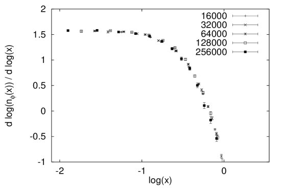
Figure 4: (a) The small $x$ behaviour of the logarithmic derivative of $n_{\varphi}(r;N)$ for the Ising model coupled to gravity. We use $N_{T}=16000$–$256000$ and $x$ is obtained by using $d_{h}=4.13$, $a=0.45$. (b) Same for the three–states Potts model coupled to gravity. We use now $d_{h}=4.27$ and $a=0.35$.

The calculation of the logarithmic derivative is performed by using a 9 point Savitzky–Golay smoothing filter [30] with a ${\rm 8}^{\rm th}$ order interpolating polynomial. The errors are computed by binning our data. The use of the filter improves the computation of the derivatives, especially near the origin. The analysis of the logarithmic derivatives provides an excellent pictorial way for realizing the scaling given by Eq. (63) near the origin. Fig. 3 shows no such scaling if $a=0.0$. Similar lack of scaling for $a=0.0$ is observed for all correlation functions we analyzed near the origin. There is an optimal value of $a$, however, where scaling becomes manifest. This is shown in Fig. 3 and Fig. 4. In order to determine the optimal $a$ we use direct fits to Eq.(63). The results are shown in Table 5 and Table 6. In order for the correlation functions to have a “smooth” continuum limit [27] it is very important that the value of $d_{h}$ extracted from those fits is the same as the one extracted from the analysis of Eq. (62) since in principle the two values can be different. For $n_{1}(r;N)$, $d_{h}$ extracted from finite size scaling variable $x$ corresponds to $d_{H}$ of Eq. (20) and $d_{h}$ extracted from the small distance behaviour corresponds to $d_{h}$ of Eq. (17). In the case of $n_{\varphi}(r;N)$, agreement between the two values implies also the existence of a diverging correlation length for the matter fields [11, 12], a fundamental assumption for scaling in critical phenomena. For matter systems coupled to gravity we could find the situation where, despite the fact that we have a continuous phase transition, the scale associated with the geometry diverges whereas the scale associated with matter does not, as is the case of many Ising spins coupled to two–dimensional quantum gravity [14]. From our results we conclude that we do obtain the same scaling exponents in Eq. (62) and Eq. (63), the small differences being attributed to finite size effects. We also observe that by introducing the shift $a$, scaling at small $x$ with reasonable values for $d_{h}$ appears from the analysis of much smaller lattices than it was thought it would be necessary before. Our results on the largest lattices are, however, necessary in order to gain confidence that the fits are stable with respect to changing the points that one includes in the fits. $d_{h}$ decreases slightly by removing points from the origin, but the fits are more stable for the largest lattice that we use.

At this point we would like to present our results for the ordinary spin–spin correlation function $G_{\varphi}(r;N)$. It is a pleasent surprise that it exhibits excellent scaling properties, in fact better than the “unnormalized” function $n_{\varphi}(r;N)$. The reason for the improved quality is presumable that some correlated fluctuations in spin and geometry are cancelled in $G_{\varphi}(r;N)$. Our results for the value of $d_{h}$ obtained from $n_{\varphi}(r;N)$ are confirmed and give us further confidence on the existence of a diverging correlation length for the matter fields. Recall that we expect the scaling

$$G_{\varphi}(r;N)\sim N^{-\Delta}g_{\varphi}(x)\,,$$ (65)

where

$$g_{\varphi}(x)\sim x^{-d_{h}\Delta}\,,\qquad x\ll 1\,.$$ (66)

In Fig. 5 we see that the scaling (65) holds very well if one chooses the appropriate value of $a$. $g_{\varphi}(x)$ has a stronger dependence on $a$ near the origin than $F_{1,\varphi}(x)$ and we do not obtain good scaling at $a=0$. The value of $a$ chosen in the plots is taken from the fits to Eq. (66). The results of the latter are shown in Table 7. As one can see from the plot of the logarithmic derivative of $g_{\varphi}(x)$ in Fig. (6), the fits are stable over a wider range than those of Eq. (63) for $n_{\varphi}(r;N)$ and we get and excellent agreement with the value of $d_{h}$ we have obtained so far. In Table 7 we show our results for different cuts for the range in $r$: We compare the same range used in Table 6 where applicable, a typical point in the region of stability and finally the point where $\chi^{2}$ becomes of order $1$. This result further supports the statement that the correlation length for the spin–spin correlation function diverges at the critical temperature.

The results for the Hausdorff dimension are further tested by measuring the loop length distribution $\rho_{N}(r,l)$ and calculating

$$\langle{l^{n}(r)}\rangle_{N}\sim N^{\frac{2n}{d_{h}}}F_{n}(x)\,,\qquad n=2,3,4\,,$$ (67)

where

$$F_{n}(x)\sim x^{2n}\,,\qquad x\ll 1\,.$$ (68)

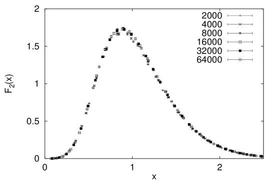
Figure 7: (a) The $\langle{l^{2}(r)}\rangle_{N}$ distributions for pure gravity rescaled according to Eq. (60) using $d_{h}=3.88$, $a=0.00$. (b) Same as in (a) for the Ising model coupled to gravity. $x$ is scaled using $d_{h}=3.99$, $a=0.0$. (c) Same as in (b) for the three–states Potts model coupled to gravity. $x$ is scaled using $d_{h}=4.07$, $a=0.0$.

We have analyzed Eq. (67) in a similar way we have analyzed $n_{1,\varphi}(r;N)$ by collapsing the distributions. In Fig. 7 we show the collapsed $\langle{l^{2}(r)}\rangle_{N}$ function and we observe that scaling holds very convincingly. Quite similar plots can be obtained for $\langle{l^{3,4}(r)}\rangle_{N}$. We observe that the extracted $d_{h}(a)$ has a very weak dependence on the shift $a$ contrary to what we found for $\langle{l^{1}(r)}\rangle_{N}$ before. This is shown in Fig. 8 for the Ising model. Similar graphs can be obtained for all models and moments and we show representative values of $d_{h}(a)$ in Table 3. In Table 4 we show the best value for the shift $a$ and the corresponding value $d_{h}(a)$. This is slightly different than the procedure we followed in the analysis of $n_{1,\varphi}(r;N)$, since now $d_{h}(a)$ is not invertible. In Fig. 6 we show that the scaling of Eq. 60 holds very well near the $r$ origin.

Finally in Fig. 10 – Fig. 12 we show our results for the loop–length distribution function $\rho_{N}(r,l)$. In Fig. 10 we show the pure gravity measurements together with a fit to Eq. (31). In the fit we simply rescale $y$ and $\rho_{N}(r,l)r^{2}$, but we otherwise keep the same coefficients as in Eq. (31). The data is consistent with the theoretical prediction, as was found before in [19], but unfortunately it has no predictive power to determine convincingly the terms in Eq. (31) for $c\not=0$. We are able to check, however, some of the scaling properties of $\rho_{N}(r,l)r^{2}$: The part of the curve corresponding to the continuum behaviour is independent of $N$ and that $\rho_{N}(r,l)(r/N^{1/d_{h}})^{2}=N^{0}F_{\rho}(y,L/N^{2/d_{h}})$ for all values of $y$ and $L/N^{2/d_{h}}$. This is shown in Fig. 13 for the three–states Potts model. It is also curious that in the range in $y$ where we observe continuum behaviour, $\rho_{N}(r,l)r^{2}$ seems to be independent of $m=2,3,5$. In this range the data points in Fig. 11 are within statistical error on top of each other. One could be tempted to conjecture that the fractal properties of space–time for unitary theories with $0\leq c<1$ are independent of $c$. In the same figure, however, we observe that the finite size corrections do depent on $c$ and it is not so clear which is the borderline in the range in $y$ where we observe continuum physics and where finite size effects are important. In contrast, for the $c=-2$ model simulated in [9, 10] we see a clear difference from our data, reflecting the fact that in this model the fractal dimension of space–time is $3.58(4)$. In Fig. 12 we compare our data with that of [9, 10].

4 Discussion

In this work we have measured the Hausdorff dimension $d_{h}$ for $0\leq c<1$ matter coupled to two–dimensional quantum gravity using various scaling arguments. In the spirit of [6], we introduced the shift $a$ in the investigation, which as a finite size correction, improves dramatically the scaling of correlation functions for small geodesic distances $r$ giving consistent results for $d_{h}$. For finite size scaling, the shift must be included in the analysis, even when we use the link distance in the definition of correlation functions, and can be used to estimate the systematic errors introduced by finite size effects. Its effect is greatest in the case of the two point functions $n_{1,\varphi}(r;N)$ and $G_{\varphi}(r;N)$. By studying the scaling behaviour of the spin–spin correlation functions we verified and extended the results of [11, 12] on the existence of a diverging correlation length for matter. We also verified the scaling properties of the moments $\langle{L^{n}}\rangle$ for pure gravity predicted in [3, 9] and found that similar scaling holds for $0<c<1$ matter coupled to gravity. We measured the loop–length distribution function $\rho_{N}(r,l)$ and showed that in the continuum limit $\rho_{\infty}(R,L)$ is not or very little affected by the back reaction of $0<c<1$ matter to gravity.

The results of our measurements of $d_{h}$ are consistent with the earlier observations in [5, 6] that the presence of $0<c<1$ matter has no or very small effect on $d_{h}$. This is in contradiction with the analytic result $d_{h}=2m$, as was mentioned in the introduction. It has been argued that the reason for the apparent contradiction is that a large Hausdorff dimension $d_{h}=2m$, $m=3,5,\ldots$ implies a very small linear extension $N^{1/d_{h}}$ for the range of $N$ accessible in the numerical simulations. However, if this argument was correct it would be very hard to understand how one can measure with excellent precision the correct KPZ exponents for the Ising and three-states Potts models from the integrated correlators. Moreover the correct scaling of the correlation functions defined in terms of geodesic distance provide even stronger evidence that we see the correct coupling of matter to the geometry in the simulations, including the fractal properties of the metric. If the linear size of the systems were much too small one should not be able to observe the correct critical behavior of conformal matter fields coupled to quantum gravity. Moreover, as it was already mentioned, it is known [13, 9, 10] that $d_{h}=2m$ is inconsistent with numerical simulations on the $c=-2$ model coupled to gravity, which corresponds to $m=1$, i.e. $d_{h}=2$. In this case the simulated systems have a quite large linear size.

As it was mentioned in the introduction the alternative prediction coming from scaling arguments for the diffusion equation in Liouville theory,

$$d_{h}=2\times\frac{\sqrt{25-c}+\sqrt{49-c}}{\sqrt{25-c}+\sqrt{1-c}},$$ (69)

is in excellent agreement with the $c=-2$ simulations, and it agrees with the rigorously established result $d_{h}=4$ for $c=0$.

Our simulations are consistent with the $d_{h}=4$ conjecture [5, 6] for Ising and three–states Potts model, especially when looking at correlators not involving the matter fields. Although the reader can draw her/his own conclusions from our measurements, we included a summary of our results in Table 8 where we display the most probable range for $d_{h}$ as measured by the different scaling arguments we used in this article. We observe that the values of $d_{h}$ coming from correlation functions involving matter fields are consistently higher. The errors are big enough to include $d_{h}=4$ within 1–1.5$\sigma$ and one can argue that finite size effects are bigger in this case: As pointed out in [5], the scaling behaviour of the spin–spin correlation function $n_{\phi}(r;N)$ is the difference $f_{1}(r)-1/(q-1)f_{2}(r)$ of the correlators $f_{1}(r)$ and $f_{2}(r)$ which count the number of like and different spins at distance $r$. They both scale identically as $n_{1}(r;N)$ and the scaling behaviour of $n_{\varphi}(r;N)$ is obtained by exact cancellation of the leading terms. In favour with the $d_{h}=4$ conjecture is our result that $\rho_{N}(r,l)$ seems to be independent of $m$ in the region where it exhibits continuum behaviour.

One, however, cannot claim that our simulations exclude the prediction of Eq. (69). Except for $n_{1}(r;N)$, one can see that $d_{h}$ increases slightly with $m$, although the signal is not clear enough to allow for a clear distinction. There exist the possibility that the larger values of $d_{h}$ obtained from $n_{\phi}(r;N)$ and $G_{\phi}(r;N)$ are a true signal. Firstly, it is of course interesting that the central values of $d_{h}$ actually agree with Eq. (69), although with large error bars. Secondly, one cannot exclude with certainty the possibility that simulations on larger lattices will not shift slightly the values of $d_{h}$ extracted from the other observables to the ones of Eq. (69). In this connection one should bear in mind that the finite size effects for the Ising and the three-states Potts model are larger than for for pure gravity, as shown in [24]. Nevertheless one can hope that future simulations might decrease systematic errors to the point that one will be able to reject convincingly at least one of the above predictions.

As we noted in the introduction, the Hausdorff dimension comes from the cutoff dependence as $L\to 0$ of the integral (32). The cutoff dependence disappears in the integrals (33) for $n>1$ and one obtains the scaling (34)-(35) which seems very well satisfied also in the case of the Ising and three-states Potts model coupled to gravity, as well as for $c=-2$! Therefore, in order to be able to fully understand the concept of the Hausdorff dimension for $c\not=0$, one needs to provide an explanation of expressions like Eq.(30) and (31) for the loop length distribution function $\rho_{V}(R,L)$, but with different powers of $y$, also for $c\neq 0$.

Acknowledgments

K.A. would like to acknowledge interesting discussions with Gudmar Thorleifsson. J.A. acknowledges the support of the Professor Visitante Iberdrola grant and the hospitality at the University of Barcelona, where part of this work was done.

$m$	$d_{h}$	$a$	$N_{T}$
2	4.05(8)	0.60(20)	8000	–	64000
3	4.11(10)	0.48(28)	16000	–	128000
5	4.01(9)	0.15(26)	16000	–	128000
2	4.05(15)	0.70(60)	16000	–	64000
3	4.11(11)	0.50(40)	32000	–	128000
5	3.98(15)	0.00(60)	32000	–	128000

Table 1: The Hausdorff dimension $d_{h}$ as determined from collapsing the $n_{1}(r;N)$ correlation functions for pure gravity ($m=2$), Ising ($m=3$) and three–states Potts model ($m=5$) coupled to gravity.

$m$	$d_{h}$	$a$	$N_{T}$
3	4.28(17)	0.60(30)	8000	–	128000
5	4.46(33)	0.53(51)	8000	–	128000
3	4.26(26)	0.56(48)	16000	–	128000
5	4.45(40)	0.55(95)	16000	–	128000

Table 2: The Hausdorff dimension $d_{h}$ as determined from collapsing the $n_{\varphi}(r;N)$ correlation functions for pure gravity Ising ($m=3$) and three–states Potts model ($m=5$) coupled to gravity.

	$d_{h}$
$n$	$m=2$		$m=3$		$m=5$
	$a=0.00$	$a=0.25$	$a=0.00$	$a=0.25$	$a=0.00$	$a=0.25$
2	3.88(3)	3.90(3)	3.99(4)	4.01(4)	4.07(3)	4.10(3)
3	3.94(3)	3.96(3)	4.06(4)	4.09(4)	4.15(4)	4.17(4)
4	3.95(3)	3.97(3)	4.08(4)	4.10(4)	4.16(4)	4.18(4)

Table 3: The Hausdorff dimension $d_{h}(a)$ as determined from collapsing the $\langle{l^{n}(r)}\rangle_{N}$ distributions for $N_{T}=16000$, $32000$ and $64000$ for pure gravity ($m=2$), Ising ($m=3$) and three–states Potts model ($m=5$) coupled to gravity.

$n$	$m=2$		$m=3$		$m=5$
	$d_{h}$	$a$	$d_{h}$	$a$	$d_{h}$	$a$
$N_{T}=16000$–$64000$
2	3.88(3)	0.00(15)	4.00(4)	0.0(3)	4.08(3)	0.0(3)
3	3.94(3)	0.0(2)	4.08(4)	0.0(4)	4.16(4)	0.1(3)
4	3.95(3)	0.00(15)	4.10(4)	0.0(5)	4.17(4)	0.1(4)
$N_{T}=4000$–$64000$
2	3.86(2)	0.00(10)	3.98(4)	0.05(10)	4.07(4)	0.12(10)
3	3.92(2)	0.05(10)	4.05(4)	0.07(18)	4.16(3)	0.15(15)
4	3.92(2)	0.05(10)	4.06(5)	0.10(18)	4.17(3)	0.13(15)

Table 4: The Hausdorff dimension $d_{h}(a)$ as determined from collapsing the $\langle{l^{n}(r)}\rangle_{N}$ correlation functions for pure gravity ($m=2$), Ising ($m=3$) and three–states Potts model ($m=5$) coupled to gravity. The best value for the shift $a$ and the corresponding $d_{h}(a)$ is recorded.

$m$	$N_{T}$	$d_{h}$	$a$	$C$	$\chi^{2}$	$r_{min}$	$r_{max}$
3	256000	4.081(4)	0.514(4)	1.049(9)	3.7	1	6
	128000	4.098(7)	0.529(5)	1.01(1)	2.1	1	5
	64000	4.080(5)	0.517(4)	1.06(1)	6.1	1	4
	32000	4.041(6)	0.492(5)	1.11(1)	7.4	1	4
	16000	3.969(9)	0.448(7)	1.25(2)	8.6	1	4
	256000	4.028(7)	0.447(9)	1.19(2)	1.3	2	7
	128000	3.994(7)	0.417(9)	1.27(2)	1.8	2	6
	64000	3.961(8)	0.39(1)	1.36(3)	1.7	2	5
	32000	3.86(1)	0.30(1)	1.65(4)	5.1	2	5
	16000	3.68(1)	0.14(2)	2.33(7)	6.7	2	5
5	256000	4.096(5)	0.482(5)	1.07(1)	3.5	1	6
	128000	4.082(4)	0.482(5)	1.07(1)	7.4	1	5
	64000	4.087(5)	0.481(4)	1.08(1)	6.9	1	4
	32000	4.042(7)	0.453(6)	1.17(2)	7.0	1	4
	16000	3.964(4)	0.406(4)	1.32(1)	42	1	4
	256000	4.031(9)	0.40(1)	1.25(3)	1.2	2	7
	128000	3.990(7)	0.367(9)	1.36(2)	2.6	2	6
	64000	3.950(9)	0.34(1)	1.46(3)	2.1	2	5
	32000	3.83(1)	0.24(1)	1.82(5)	4.3	2	5
	16000	3.627(8)	0.051(9)	2.69(5)	30	2	5
2	128000	4.01(1)	0.542(9)	1.04(3)	0.8	1	5
	64000	4.023(6)	0.551(5)	1.06(1)	3.9	1	4
	32000	4.01(1)	0.54(1)	1.09(3)	1.6	1	4
	16000	3.94(2)	0.49(1)	1.23(4)	1.5	1	4
	128000	3.95(2)	0.47(2)	1.25(5)	0.2	2	5
	64000	3.920(9)	0.44(1)	1.34(4)	0.8	2	5
	32000	3.84(2)	0.35(3)	1.58(8)	0.4	2	5
	16000	3.69(3)	0.22(3)	2.1(1)	1.8	2	5

Table 5: The results of the fits to Eq. (63) for $n_{1}(r;N)$ for pure gravity ($m=2$), Ising ($m=3$) and three–states Potts ($m=5$) model coupled to gravity.

$m$	$N_{T}$	$c$	$a$	$C$	$d_{h}$	$\chi^{2}$	$r_{min}$	$r_{max}$
3	256000	1.75(2)	0.46(2)	0.73(3)	4.13(3)	0.26	1	6
	128000	1.74(2)	0.43(2)	0.76(2)	4.10(2)	0.56	1	5
	64000	1.72(2)	0.42(2)	0.77(2)	4.08(3)	0.44	1	4
	256000	1.68(3)	0.30(7)	0.87(7)	4.01(5)	0.26	2	7
	128000	1.62(3)	0.21(6)	0.97(6)	3.94(4)	0.74	2	6
	64000	1.58(3)	0.16(7)	1.04(8)	3.87(5)	0.21	2	5
5	256000	1.56(2)	0.35(2)	0.73(2)	4.27(3)	1.15	1	6
	128000	1.56(1)	0.36(2)	0.73(2)	4.27(2)	0.81	1	5
	64000	1.57(2)	0.38(2)	0.71(2)	4.28(3)	0.67	1	4
	256000	1.43(3)	0.07(7)	0.97(6)	4.06(5)	0.46	2	7
	128000	1.43(3)	0.08(6)	0.98(6)	4.05(5)	0.85	2	6
	64000	1.36(3)	-0.03(7)	1.10(7)	3.93(5)	0.88	2	5

Table 6: The results of the fits to Eq. (63) for $n_{\varphi}(r;N)$ for Ising ($m=3$) and three–states Potts ($m=5$) model coupled to gravity.

$m$	$N_{T}$	$c$	$a$	$C$	$d_{h}$	$\chi^{2}$	$r_{min}$	$r_{max}$
3	256000	1.32(2)	0.51(4)	0.49(2)	3.97(6)	0.13	1	6
		1.34(1)	0.53(3)	0.50(1)	4.00(4)	0.15	1	9
		1.37(1)	0.59(2)	0.54(1)	4.10(3)	1.3	1	13
		1.38(2)	0.66(8)	0.56(4)	4.13(7)	0.14	2	11
		1.44(2)	0.86(7)	0.66(4)	4.32(6)	1.5	2	14
	128000	1.35(2)	0.56(4)	0.52(2)	4.03(7)	0.07	1	5
		1.38(1)	0.61(3)	0.55(2)	4.14(4)	0.47	1	8
		1.40(1)	0.65(2)	0.58(1)	4.20(3)	1.2	1	10
		1.44(3)	0.81(8)	0.65(4)	4.32(8)	0.26	2	9
		1.51(2)	1.02(7)	0.77(4)	4.53(6)	1.8	2	12
	64000	1.35(2)	0.54(3)	0.51(2)	4.05(5)	0.15	1	5
		1.39(1)	0.61(2)	0.55(1)	4.16(3)	1.9	1	8
5	256000	1.57(2)	0.55(3)	0.47(2)	3.93(5)	0.08	1	6
		1.59(1)	0.59(3)	0.50(2)	4.00(3)	0.54	1	9
		1.63(1)	0.64(2)	0.53(1)	4.06(3)	1.6	1	11
		1.67(3)	0.79(8)	0.61(4)	4.18(7)	0.53	2	10
		1.73(2)	0.94(7)	0.70(5)	4.33(6)	1.7	2	12
	128000	1.55(2)	0.53(3)	0.46(2)	3.86(5)	5.1$\times{\rm 10}^{\rm-3}$	1	5
		1.57(1)	0.57(2)	0.48(1)	3.93(3)	0.67	1	8
		1.59(1)	0.60(2)	0.50(1)	3.98(3)	1.7	1	9
		1.61(3)	0.68(8)	0.53(4)	4.03(7)	0.42	2	8
		1.65(3)	0.77(7)	0.58(4)	4.12(6)	1.1	2	9
	64000	1.55(2)	0.53(3)	0.45(2)	3.87(4)	0.43	1	5
		1.60(1)	0.61(2)	0.51(1)	4.01(3)	2.9	1	7

Table 7: The results of the fits to Eq. (66) for the normalized spin–spin correlation function for Ising ($m=3$) and three–states Potts ($m=5$) model coupled to gravity.

$d_{h}$
$m=2$	$m=3$	$m=5$	Method
4.05(15)	4.11(10)	4.01(9)	$n_{1}(r;N)$	FSS
3.92–4.01	3.99–4.08	3.99–4.10	$n_{1}(r;N)$	SDS
3.85–3.98	3.96–4.14	4.05–4.20	$\langle{l^{n}(r)}\rangle_{N}$	FSS
	4.28(17)	4.46(33)	$n_{\varphi}(r;N)$	FSS
	3.90–4.16	4.00–4.30	$n_{\varphi}(r;N)$	SDS
	3.96–4.38	3.97–4.39	$G_{\varphi}(r)_{N}$	SDS

Table 8: A summary of the results for $d_{h}$ shown in Table 3–Table 7. FSS in the Method column stands for Finite Size Scaling and SDS for Small Distance Scaling.

Figure 1: (a) $d_{h}(a)$ from collapsing $n_{1}(r;N)$ for $N_{T}=8000$–$64000$ for pure gravity. Data is collapsed in groups of three lattice sizes and in the graph we indicate the largest of each group. We show the errors computed from $\chi^{2}$ only for the largest lattice in order to simplify the graph. The errors for the smaller lattices are quite similar. (b) Same as in (a) for the Ising model for $N_{T}=8000$–$128000$. (c) Same as in (b) for the three–states Potts model.

Figure 2: (a) $d_{h}(a)$ from collapsing $n_{\varphi}(r;N)$ for $N_{T}=8000$–$128000$ for the Ising model the same way as described in Fig. 1. (b)Same as in (a) for the three–states Potts model.

Figure 3: (a) The small $x$ behaviour of the logarithmic derivative of $n_{1}(r;N)$. We use $N_{T}=32000$–$128000$, $d_{h}=4.02$ and $a=0,0.54$. (b) Same as in (a) for the Ising model coupled to gravity. We plot for $N_{T}=64000$–$256000$, $a=0,0.51$ and $d_{h}=4.08$. (c) Same as in (b) for the three–states Potts model coupled to gravity where $a=0,0.48$ and $d_{h}=4.10$.

Figure 5: (a) The rescaled according to Eq. (65) normalized spin–spin correlation function $g_{\varphi}(r;N)$ for the Ising model coupled to gravity. We use $N_{T}=2000$–$256000$, $d_{h}=4.0$, $a=0.51$. (b) Same for the three–states Potts model coupled to gravity. We use $a=0.55$.

Figure 6: (a) The small $x$ behaviour of the logarithmic derivative of the rescaled normalized spin–spin correlation function $g_{\varphi}(r;N)$ for the Ising model coupled to gravity. We use $N_{T}=16000$–$256000$ and $x$ is obtained by using $d_{h}=4.0$, $a=0.51$. (b) Same for the three–states Potts model coupled to gravity. We use now $d_{h}=4.0$ and $a=0.55$.

Figure 8: $d_{h}(a)$ from collapsing $\langle{l^{2}(r)}\rangle_{N}$ for $N_{T}=16000$–$64000$ for the Ising model coupled to gravity.

Figure 9: (a)The small $x$ behaviour of the logarithmic derivative for pure gravity for $\langle{l^{n}(r)}\rangle_{N}$ for $N_{T}=2000$–$64000$. (b) Same as in (a) for the Ising model coupled to gravity and (c) for the three–states Potts model coupled to gravity.

Figure 10: The loop length distribution function for pure gravity for $N_{T}=64000$. The dashed line is a fit to Eq. (31).

Figure 11: (a) The loop length distribution function for the Ising model for $N_{T}=64000$ shown together with the pure gravity one. A wider range in $y$ is included in the plot in order to show the $m$–dependence in the areas where finite size effects are important. (b) same as in (a) for the three–states Potts model.

Figure 12: The loop length distribution function for pure gravity ($c=0$) and the $c=-2$ model for $N_{T}=64000$. The data for the $c=-2$ model is taken from [10].

Figure 13: (a)The loop length distribution function for the three–states Potts model coupled to gravity for $N_{T}=64000$ and $32000$ for fixed $l$. (b) The same, but for (approximately) fixed $l/N^{2/d_{h}}$ for $d_{h}=4.0$. Similar plots are obtained for pure gravity and the Ising model coupled to gravity.

References

- [1] V. Knizhnik, A. Polyakov and A. Zamolodchikov, Mod.Phys.Lett A3 (1988) 819.
- [2] F. David, Mod.Phys.Lett. A3 (1988) 1651; J. Distler and H. Kawai, Nucl.Phys. B321 (1989) 509.
- [3] H. Kawai, N. Kawamoto, T. Mogami and Y. Watabiki Phys.Lett. B306 (1993) 19.
- [4] J. Ambjørn and Y. Watabiki, Nucl.Phys. B445 (1995) 129.
- [5] S. Catterall, G. Thorleifsson, M. Bowick and V. John, Phys.Lett. B354(1995) 58.
- [6] J. Ambjørn, J. Jurkiewicz and Y. Watabiki, Nucl.Phys. B454 (1995) 313.
- [7] J. Distler, Z. Hlousek and H. Kawai, Int. J. Mod. Phys. A5 (1990) 1093.
- [8] J. Ambjørn, B. Durhuus and J. Fröhlich, Nucl.Phys. B257 (1985) 433; B270 (1986) 457; B275 (1986) 161-184; J. Ambjørn, B. Durhuus J. Fröhlich and P. Orland, B270 (1986) 457; B275 (1986) 161; F. David, Nucl.Phys. B257 (1985) 45; Nucl.Phys. B257 (1985) 543; V.A. Kazakov, I. Kostov and A.A. Migdal, Phys.Lett. B157 (1985) 295; Nucl.Phys. B275 (1986) 641.
- [9] J. Ambjørn, K. Anagnostopoulos, L. Jensen, T. Ichihara, N. Kawamoto, K. Yotsuji and Y. Watabiki, “Quantum Geometry of Topological Gravity”, NBI-HE-96-64 and TIT/HEP-352 (hep–lat/9611032).
- [10] J. Ambjørn, K. Anagnostopoulos, L. Jensen, T. Ichihara, N. Kawamoto, K. Yotsuji and Y. Watabiki, to appear.
- [11] J. Ambjørn, K. Anagnostopoulos, U. Magnea and G. Thorleifsson, Phys.Lett. B388 (1996) 713.
- [12] J. Ambjørn, K. Anagnostopoulos, U. Magnea and G. Thorleifsson, “Spin-spin correlation functions of spin systems coupled to 2-d quantum gravity for ”, NBI-HE-96-44 (hep–lat/9608022).
- [13] N. Kawamoto, V.A. Kazakov, Y. Saeki and Y. Watabiki, Phys. Rev. Lett. 68 (1992) 2113.
- [14] M. G. Harris and J. Ambjørn, Nucl.Phys. B474 (1996) 575.
- [15] F. David, Nucl.Phys. B368 (1992) 671.
- [16] N. Kawamoto, Y. Saeki and Y. Watabiki, unpublished; Y. Watabiki, Progress in Theoretical Physics, Suppl. No. 114 (1993) 1; N. Kawamoto, In Nishinomiya 1992, Proceedings, Quantum gravity, 112, ed. K. Kikkawa and M. Ninomiya (World Scientific); In First Asia-Pacific Winter School for Theoretical Physics 1993, Proceedings, Current Topics in Theoretical Physics, ed. Y.M. Cho (World Scientific).
- [17] Y. Watabiki, Nucl.Phys. B441 (1995) 119; Progress of Theoretical Physics, Suppl. 114 (1993) 1.
- [18] N. Ishibashi and H. Kawai, Phys.Lett. B314 (1993) 190; Phys.Lett. B322 (1994) 67; M. Fukuma. N. Ishibashi, H. Kawai and M. Ninomiya, Nucl.Phys. B427 (1994) 139.
- [19] N. Tsuda and T. Yukawa, Phys. Lett. B305 (1993) 223; A. Fujitsu, N. Tsuda and T. Yukawa, “2D Quantum Gravity -Three States of Surfaces-, KEK-CP-029 (hep-lat/9603013).
- [20] J. Ambjørn, B. Durhuus and T. Jonsson, Phys.Lett. B244 (1990) 403; Mod.Phys.Lett. A6 (1991) 1133.
- [21] J. Jurkiewicz, A. Krzywicki, B. Petersson and B. Soderberg, Phys.Lett. B213 (1988) 511; C.F. Baillie and D.A. Johnston, Phys.Lett. B286 (1992) 44; S. Catterall, J. Kogut and R. Renken, Phys.Lett. B292 (1992) 277; J. Ambjørn, B. Durhuus, T. Jonsson and G. Thorleifsson, Nucl.Phys. B398 (1993) 568.
- [22] J. Ambjørn, G. Thorleifsson and M. Wexler, Nucl.Phys. B439 (1995) 187.
- [23] H. Aoki, H. Kawai, J. Nishimura and A. Tsuchiya, Nucl.Phys. B474 (1996) 512.
- [24] N.D. Hari Dass, B.E. Hanlon and T. Yukawa, Phys.Lett. B368 (1996) 55.
- [25] D.V. Boulatov and V.A. Kazakov, Phys.Lett. B184 (1987) 247.
- [26] J. M. Daul, “–states Potts Model on a Random Planar Lattice”, LPTENS 94 (hep–th/9502014).
- [27] Y. Watabiki, “Fractal Structure of Space–Time in Two-Dimensional Quantum Gravity”, TIT/HEP-333 (hep-th/9605185).
- [28] G.K. Savvidy and N.G. Ter-Arutyunyan Savvidy, EPI-865-16-86 (1986); J. Comput. Phys. 97 (1991) 566; N.Z. Akopov, G.K. Savvidy and N.G. Ter-Arutyunyan Savvidy, J. Comput. Phys. 97 (1991) 573.
- [29] M. Lüscher, Comput. Phys. Commun. 79 (1994) 100; F. James, Comput. Phys. Commun. 79 (1994) 111; Erratum 97 (1996) 357.
- [30] A. Savitsky and M.J.E. Golay, Analytic Chemistry 36 (1964) 1627; W.H. Press S.A. Teukolsky, W.T. Vetterling and B.P. Flannery, “Numerical Recipes in C”, ed., Cambridge University Press.