Perturbation theory predictions and Monte Carlo simulations for the 2-$d$ $O(n)$ non-linear $\sigma$-models

Abstract

By using the results of a high-statistics (${\cal O}(10^{7})$ measurements) Monte Carlo simulation we test several predictions of perturbation theory on the $O(n)$ non-linear $\sigma$-model in 2 dimensions. We study the $O(3)$ and $O(8)$ models on large enough lattices to have a good control on finite-size effects. The magnetic susceptibility and three different definitions of the correlation length are measured. We check our results with large-$n$ expansions as well as with standard formulae for asymptotic freedom up to 4 loops in the standard and effective schemes. For this purpose the weak coupling expansions of the energy up to 4 loops for the standard action and up to 3 loops for the Symanzik action are calculated. For the $O(3)$ model we have used two different effective schemes and checked that they lead to compatible results. A great improvement in the results is obtained by using the effective scheme based on the energy at 3 and 4 loops. We find that the $O(8)$ model follows very nicely (within few per mille) the perturbative predictions. For the $O(3)$ model an acceptable agreement (within few per cent) is found.

I Introduction

According to perturbation theory $(PT)$, the $O(n)$ non-linear $\sigma$-model in 2 dimensions for $n\geq 3$ resembles Yang-Mills theories in 4 dimensions. Both are asymptotically free [1, 2] and present a spontaneous generation of mass. Moreover for $n$=3 the model has a non-trivial topological content [3]. Consequently these models are considered as good toy models for testing methods and solutions in 4-dimensional Yang-Mills theories. In condensed matter physics these models have applications in the study of ferromagnetic systems.

There is an extensive literature devoted to investigate the validity of $PT$ in these models on the lattice and in particular the onset of scaling (see for instance [4, 5, 6, 7, 8]). In [4, 5] the $O(3)$ model was analyzed by using improved actions. The obtained results still differ from the exact calculated mass-gap [9, 10] by $\sim 15\%$. In [5] the authors made use of the perturbative $\beta$ function up to 3 loops [11]. In [6, 7] faster updating algorithms were used. The mass-gap for the $O(3)$ model was calculated in [6] by using the standard action and an overrelaxed algorithm. Up to a correlation length $\sim 300$ (in units of lattice spacings) it showed a deviation from the exact result [9] of about 20%. The $O(4)$ and $O(8)$ models with standard action were studied in [7] by using the cluster algorithm [12]. The deviation from the exact result for the $O(8)$ model at correlation lengths $\sim 30$ was a few per cent. In [8] an analysis of the performance of different lattice geometries for the standard action of the $O(3)$ model was presented. There was no clear signal of an earlier onset of asymptotic scaling.

The use of $PT$ for such models is not guaranteed. The Mermin-Wagner theorem [13] states that continuous symmetries in 2-dimensional theories cannot be spontaneously broken. Therefore $PT$, which is an expansion around a trivial vacuum, is not a priori well-founded. Motivated by this observation and by the lack of clear asymptotic scaling in the previous literature, it has been argued [14] that all $O(n\geq 2)$ models undergo a Kosterlitz-Thouless $(KT)$ [15, 16] phase transition at some finite beta $\beta_{KT}$.

In the present work we have performed a high-statistics simulation (${\cal O}(10^{7})$ measurements) for the $O(3)$ and $O(8)$ models on the lattice up to correlations $\sim 130$ for the $O(3)$ model and $\sim 70$ for the $O(8)$ model. For the $O(3)$ model we have used the tree-level improved Symanzik action [17] and for the $O(8)$ model the standard action. We have measured the magnetic susceptibility and three different definitions of the correlation length and compared the results with both the $PT$ and $KT$ set of predictions. We have computed also some scaling ratios which are particularly sensitive to the $PT$ versus $KT$ scenarios. We have made use of the corrections to asymptotic scaling in $PT$ up to 4 loops in both the standard and effective schemes [18] for the $O(8)$ model and up to 3 loops for the $O(3)$ model. An effective scheme can be defined by using any short distance dominated operator; we have used the density of energy operator [18]. Hereafter we will call it indistinctly effective or energy scheme. To include the analysis in this energy scheme, new analytic results are reported in this paper: the 4-loop coefficient in the weak coupling expansion of the energy for the standard action and the complete calculation of all coefficients up to 3 loops for the Symanzik action.

We have used two different definitions of energy operators for the Symanzik action and checked that the corresponding effective schemes agree. Lacking a rigorous treatment for these schemes, this check becomes an important test.

We have avoided strong coupling effects by starting the simulations at large enough correlation lengths. The minimal correlation was $\sim 10$ for the standard action and $\sim 16$ for the tree-level Symanzik action.

We have not made use of finite-size scaling (questioned due to the validity of $PT$ whenever the limit $\rho\equiv L/\xi\rightarrow 0$ holds, where $L$ is the lattice size and $\xi$ any characteristic correlation length) and we have used rather large lattices ($\rho\approx 7-10$) in order to control the finite-size effects. We have checked that the finite-size effects at these $\rho$ values are negligible.

We are able also to compare the large-$n$ predictions with our data. In particular, we have checked the relationship between the two correlation lengths $\xi^{\rm exp}$ and $\xi^{(2)}$ (see eq. (9) below) known up to ${\cal O}(1/n)$ and the prediction for the magnetic susceptibility, known up to ${\cal O}(1/n^{2})$.

In section 2 we will show the predictions of both $PT$ and $KT$ for the model as well as some necessary $1/n$ expansions. In section 3 we will describe our simulations and give the results while in section 4 we will compare them with the two different scenarios described in section 2. In this section we will also use the Monte Carlo data of ref. [6] for the $O(3)$ model with standard action to check the presently known 4-loop perturbative computations. Our conclusions are given in section 5. In the appendix we will show some technical details concerning the perturbative computation of the energy up to 4 loops for the standard action and up to 3 loops for the Symanzik action.

II Predicted scenarios for the $\sigma$-models

The $O(n)$ non-linear $\sigma$-model in 2 dimensions is defined formally in the continuum by the action

$$S={\beta\over 2}\int{\rm d}^{2}x(\partial_{\mu}{\vec{\phi}})^{2},$$ (1)

where ${\vec{\phi}}(x)$ is an $n$-component real scalar field, together with the constraint ${\vec{\phi}}(x)^{2}=1$ for all $x$. $\beta$ is the inverse of the bare coupling constant. On the lattice one can regularize this theory by making use of different actions. For our simulation we chose the standard action

$$S^{\rm standard}=-\beta\sum_{x,\mu}{\vec{\phi}}(x)\cdot{\vec{\phi}}(x+{\hat{\mu}})$$ (2)

and the tree-level improved Symanzik action [17]

$$S^{\rm Symanzik}=-\beta\sum_{x,\mu}\left({4\over 3}{\vec{\phi}}(x)\cdot{\vec{\phi}}(x+{\hat{\mu}})-{1\over{12}}{\vec{\phi}}(x)\cdot{\vec{\phi}}(x+2{\hat{\mu}})\right).$$ (3)

We have measured the magnetic susceptibility $\chi$ defined as the zero momentum correlation function,

$$\chi\equiv\sum_{x_{1},x_{2}}G(x_{1},x_{2}),\qquad\qquad\qquad G(x_{1},x_{2})\equiv\langle{\vec{\phi}}(0,0)\cdot{\vec{\phi}}(x_{1},x_{2})\rangle$$ (4)

where we have assumed a symmetric lattice of size $L$ with periodic boundary conditions in both directions and called $x_{1}$ and $x_{2}$ the two coordinates of the point $x$. We will need also ${\cal F}$ defined as the correlation function at the smallest lattice non-zero momentum $2\pi/L$,

$${\cal F}\equiv\left({1\over 2}\sum_{x_{1},x_{2}}{\rm e}^{2\pi ix_{1}/L}G(x_{1},x_{2})+{1\over 2}\sum_{x_{1},x_{2}}{\rm e}^{2\pi ix_{2}/L}G(x_{1},x_{2})\right).$$ (5)

We have made use also of the wall-wall correlation function defined as

$${\bar{G}}(x_{1})\equiv{1\over L}\sum_{x_{2}}G(x_{1},x_{2}).$$ (6)

We have considered three definitions of correlation lengths, the exponential one $\xi^{\rm exp}$ and the second momenta of the correlation function $\xi^{(2)}$ and $\xi^{\prime(2)}$. They are defined as $(|x|\equiv\sqrt{x_{1}^{2}+x_{2}^{2}})$

$$\xi^{\rm exp} \equiv \displaystyle\lim_{|x|\to\infty}{{-|x|}\over{\ln G(x_{1},x_{2})}},$$ (7)

$$\xi^{(2)} \equiv {\sqrt{\chi/{\cal F}-1}\over{2\sin\pi/L}},$$ (8)

$$\xi^{\prime(2)} \equiv \sqrt{{1\over 4}{{\sum^{\prime}|x|^{2}G(x_{1},x_{2})}\over{\sum G(x_{1},x_{2})}}},$$ (9)

where $\sum^{\prime}$ indicates that the sum runs over $-L/2+1\leq x_{1},x_{2}\leq L/2$. The operative definition of $\xi^{\rm exp}$ on a finite lattice was the solution of the equation

$${\bar{G}}(t_{1})\cosh\Big{(}\left(t_{2}-L/2\right)/\xi^{\rm exp}\Big{)}={\bar{G}}(t_{2})\cosh\Big{(}\left(t_{1}-L/2\right)/\xi^{\rm exp}\Big{)},$$ (10)

for big enough $t_{1}$ and $t_{2}$ where ${\bar{G}}(t)$ is the wall-wall correlation and $t_{2}-t_{1}=\Delta_{t}$ with $\Delta_{t}=1$, 2. As a function of $t_{1}$, the solution of the previous equation displays a long stable plateau for $\xi^{\rm exp}\lesssim t_{1}\lesssim 3\xi^{\rm exp}$. Anyhow, we chose the value and error for $\xi^{\rm exp}$ self-consistently at $t_{1}\approx 2\xi^{\rm exp}$. The result is independent of $\Delta_{t}$ (both for the Symanzik action and the standard one) and we selected the value $\Delta_{t}=1$. In Figure 1 we show an example of solution of eq. (10) as a function of $t_{1}$; the plateau is apparent.

On the other hand, the value for the definition $\xi^{\prime(2)}$ was extracted from the wall-wall correlation function

$$\xi^{\prime(2)}=\sqrt{{1\over 2}{{\sum^{\prime}t^{2}{\bar{G}}(t)}\over{\sum{\bar{G}}(t)}}}.$$ (11)

In the large-$L$ limit $\xi^{(2)}$ and $\xi^{\prime(2)}$ coincide. For finite $L$ the three definitions show rather different finite-size behaviours [19, 20].

FIG. 1.: Solution of eq. (10) as a function of $t_{1}$ for $\Delta_{t}=1$ for the $O(8)$ model at $\beta=4.8$ and $L=120$. The parameter $t_{1}$ is given in units of lattice spacings (external labels of the horizontal axis) and units of correlation length (internal labels).

The scaling of these quantities as predicted in perturbation theory in the large-$L$ limit is

$$\xi = C_{\xi}\left({{n-2}\over{2\pi\beta}}\right)^{\displaystyle 1\over\displaystyle{n-2}}\exp\left({\displaystyle{2\pi\beta}\over\displaystyle{n-2}}\right)\left(1+\sum_{k=1}^{\infty}{a_{k}\over\beta^{k}}\right),$$ (12)

$$\chi = C_{\chi}\left({{n-2}\over{2\pi\beta}}\right)^{\displaystyle{n+1}\over\displaystyle{n-2}}\exp\left({\displaystyle{4\pi\beta}\over\displaystyle{n-2}}\right)\left(1+\sum_{k=1}^{\infty}{b_{k}\over\beta^{k}}\right).$$ (13)

The form of the expression for $\xi$ is valid for all three definitions. The coefficients of non-universal scaling $a_{k}$ and $b_{k}$ are action-dependent. They are known up to 3 loops for the Symanzik action [11] and up to 4 loops for the standard action [21]. The constant $C_{\xi}$ is definition- and action-dependent (its dependence on the action is exactly calculable in perturbation theory up to an universal constant). $C_{\xi}$ is known exactly for the exponential definition. With the standard action it is [9, 10]

$$C_{\xi^{\rm exp}}=\left({{\rm e}\over 8}\right)^{\displaystyle 1\over\displaystyle{n-2}}\Gamma\left(1+{1\over{n-2}}\right)\;2^{-5/2}\;\exp\left(-{{\pi}\over{2(n-2)}}\right).$$ (14)

The corresponding constant in the tree-level Symanzik action is easily obtained from (14) by using the exact perturbative result [17, 22]

$${\Lambda_{\rm Symanzik}\over\Lambda_{\rm standard}}=\exp\left({{0.2964\;n-0.0920}\over{n-2}}\right).$$ (15)

The other constants are not exactly known. For the correlation lengths in the large-$n$ limit we have [21]

$$C_{\xi^{\prime(2)}}=C_{\xi^{(2)}}=C_{\xi^{\rm exp}}\left(1-{{0.0032}\over n}+{\cal O}\left({1\over n^{2}}\right)\right).$$ (16)

In the same limit the value of $C_{\chi}$ with the standard action is [23]

$$C_{\chi}=0.196\left(1-{{4.267}\over n}+{\cal O}\left({1\over n^{2}}\right)\right).$$ (17)

In ref. [24] there are numerical results for $C_{\chi}$ up to ${\cal O}(1/n^{2})$,

$$O(3) \;\;\;{\rm(standard\;action)}\;\;\longrightarrow\;\;C_{\chi}=0.0127$$ (18)

$$O(8) \;\;\;{\rm(standard\;action)}\;\;\longrightarrow\;\;C_{\chi}=0.103$$ (19)

By using eq. (15) the value of $C_{\chi}$ for the Symanzik action can be obtained; for $n=3$ it is $C_{\chi}=0.0625$. From eq. (13) we conclude that the ratio

$$R_{PT}\equiv{\chi\over\xi^{2}}\left({{2\pi\beta}\over{n-2}}\right)^{\displaystyle{n-1}\over\displaystyle{n-2}}\left(1+{\cal O}\left({1\over{\beta}}\right)\right)$$ (20)

tends to the constant $C_{\chi}/C_{\xi}^{2}$ as the continuum limit $\beta\rightarrow\infty$ is approached. The parentheses contain the corrections which are known up to 4 loops for the standard action and 3 loops for the Symanzik action. Hereafter we will call this ratio the $PT$ ratio.

The perturbative expansions of the energy for both the standard action and the Symanzik action are calculated in the appendix.

The correlation length for the $O(2)$ model, when $\tau\equiv\beta_{KT}-\beta$ is positive and small, scales as [15, 16]

$$\xi=A\exp\left({B\over\tau^{1/2}}\right),$$ (21)

with $A$ and $B$ positive constants. On the other hand the ratio

$$R_{KT}\equiv{{\chi\;\tau^{r}}\over\xi^{2-\eta}}$$ (22)

should be constant as we approach $\beta_{KT}$ from below. Here $\eta=1/4$ is the critical exponent. Following the renormalization group considerations of ref. [15, 16] one can show that $r=1/16$ [25]. Recent numerical analyses for the $O(2)$ model [26, 27, 28, 29, 30] have yielded several values for $r$ which are all consistent with the bound $|r|\lesssim 0.1$. Eqs. (21-22) are the expected behaviour (and consistent with Monte Carlo simulations) for the $O(2)$ model. From now on we will call the ratio in eq. (22) the $KT$ ratio. The $KT$ scenario for the $O(n)$ model is the extension of this behaviour for $n\geq 3$.

In ref. [28] a fit of Monte Carlo data for $\chi$ and $\xi$ for the $O(3)$ model with standard action was performed. Within errors it gave a constant for the $KT$ ratio and a strong decrease far from constant for the $PT$ ratio. We have simulated the $O(3)$ model with the tree-level Symanzik action [17] in order to check the results of ref. [28] with an action classically closer to the continuum limit.

III The Monte Carlo simulation

We have performed an extensive Monte Carlo simulation of the $O(3)$ model with Symanzik action and the $O(8)$ model with standard action. In tables I and II we show the corresponding sets of raw data. The statistical error of the three entries for $\xi^{\prime(2)}$, $\xi^{(2)}$ in table II for $L=50,100,200$ and the two entries for $L=150,300$ in table I display a strong dependence on the lattice size. This can be explained by taking into account that the definition of, for example $\xi^{\prime(2)}$, involves the quantity $\sum|x|^{2}G(x)$. For a big enough lattice the “signal” is independent on size, while the “noise” grows as the volume. A similar argument can be used for $\xi^{(2)}$.

Table I

Raw Monte Carlo data for $O(3)$ with Symanzik action. The second row for $L=300$ was used only for checks of finite-size dependence.

 $\beta$  $L$  $10^{-6}\cdot{\rm stat}$  $\chi$  $\xi^{\rm exp}$  $\xi^{(2)}$  $\xi^{\prime(2)}$  $1.40$  $150$  $8.1$  $361.41(26)$  $16.216(23)$  $16.195(17)$  $15.441(17)$  $1.40$  $300$  $8.08$  $360.99(27)$  $16.168(27)$  $16.161(71)$  $16.050(52)$  $1.45$  $200$  $8$  $587.18(44)$  $21.519(30)$  $21.443(23)$  $20.462(22)$  $1.50$  $260$  $6.24$  $972.78(83)$  $28.793(50)$  $28.730(35)$  $27.273(34)$  $1.55$  $340$  $18$  $1634.41(83)$  $38.668(61)$  $38.636(36)$  $36.410(41)$  $1.60$  $450$  $2.88$  $2777.3(3.6)$  $52.72(38)$  $52.42(10)$  $49.18(25)$  $1.65$  $600$  $4$  $4743.1(5.2)$  $71.08(34)$  $70.93(13)$  $66.27(20)$  $1.70$  $800$  $7.25$  $8125.7(6.7)$  $96.67(37)$  $96.28(13)$  $89.64(19)$  $1.75$  $1050$  $1.24$  $13852.7(27.7)$  $-$  $130.25(36)$  $-$

Table II

Raw Monte Carlo data for $O(8)$ with standard action. The first and third rows ($L=50$ and $L=200$ respectively) were used only for checks of finite-size dependence.

 $\beta$  $L$  $10^{-6}\cdot{\rm stat}$  $\chi$  $\xi^{\rm exp}$  $\xi^{(2)}$  $\xi^{\prime(2)}$  $4.6$  $50$  $16$  $145.501(77)$  $9.7787(75)$  $9.7541(40)$  $7.5678(69)$  $4.6$  $100$  $3.76$  $149.00(17)$  $9.881(14)$  $9.864(13)$  $9.533(20)$  $4.6$  $200$  $16$  $149.029(83)$  $9.8624(74)$  $9.860(35)$  $9.842(14)$  $4.7$  $110$  $16$  $177.86(10)$  $10.9156(80)$  $10.913(12)$  $10.543(13)$  $4.8$  $120$  $16$  $212.13(12)$  $12.0745(88)$  $12.071(13)$  $11.635(15)$  $4.9$  $140$  $16$  $253.11(14)$  $13.370(10)$  $13.358(17)$  $13.005(17)$  $5.0$  $160$  $40$  $302.600(85)$  $14.806(10)$  $14.788(11)$  $14.431(10)$  $5.4$  $220$  $40$  $620.78(18)$  $22.193(28)$  $22.199(15)$  $21.381(15)$  $5.8$  $340$  $65$  $1289.32(30)$  $33.526(47)$  $33.411(16)$  $32.357(21)$  $6.0$  $290$  $3.2$  $1854.6(2.5)$  $40.933(81)$  $40.879(78)$  $36.530(87)$  $6.1$  $320$  $3.2$  $2236.6(3.0)$  $45.52(10)$  $45.425(87)$  $40.49(11)$  $6.2$  $360$  $3.2$  $2689.7(3.7)$  $50.21(11)$  $50.26(10)$  $44.99(12)$  $6.3$  $390$  $3.2$  $3239.7(4.5)$  $55.77(12)$  $55.60(11)$  $49.35(14)$  $6.4$  $440$  $3.2$  $3909.8(5.4)$  $61.94(15)$  $61.75(12)$  $55.06(15)$  $6.5$  $480$  $3.2$  $4686.9(6.5)$  $68.36(17)$  $68.16(14)$  $60.64(16)$

We have updated the configurations with the Wolff algorithm [12]. We verified the absence of autocorrelations in the data for the standard action. For the Symanzik action we have used a generalization of this algorithm [31] which does not completely eliminate the critical slowing down. According to the measured integrated autocorrelation time [31], we have performed 4 decorrelating updatings for this action between successive measurements. Once these decorrelating updatings were done, we explicitly checked the absence of autocorrelations in the data for the Symanzik action. We have measured $\chi$ and the three definitions of $\xi$ shown in the previous section. The necessary two-point correlation functions were evaluated by using an improved estimator [32].

Table III

Integrated autocorrelation times $\tau^{\rm int}_{1,2}$ for the energies $E^{S}_{1,2}$ and size $\langle C_{\#}\rangle$ of the average Fortuin-Kasteleyn cluster for a Symanzik-improved action simulated on a lattice size $L=100$.

 $\beta$  $E^{S}_{1}$  $\tau^{\rm int}_{1}$  $E^{S}_{2}$  $\tau^{\rm int}_{2}$  $\langle C_{\#}\rangle$  $2.$  $0.98252(5)$  $23.6(1.6)$  $0.7788(2)$  $26.4(1.8)$  $3464.9$  $5.$  $1.14782(2)$  $29.4(2.2)$  $0.91534(4)$  $31.4(2.4)$  $6148.7$  $10.$  $1.19949(2)$  $40.4(3.5)$  $0.95812(4)$  $42.7(3.8)$  $7321.1$

We have also done a few runs at small physical volumes, $\rho=L/\xi\ll 1$, to calculate the energy for the Symanzik-improved action at large $\beta$, (see appendix). We have realised that the performance of the extension of the Wolff algorithm for Symanzik actions [31] is less effective in this regime. In Table III we give the integrated autocorrelation times $\tau^{\rm int}_{1,2}$ for the calculation of the energies $E^{S}_{1}$ and $E^{S}_{2}$ respectively on a lattice of size $L=100$ after $7\;10^{5}$ measurements for several $\beta$. The integrated autocorrelation times must be compared with the values $\tau^{\rm int}\sim 4$ found when $\rho\gg 1$ [31]. In table III we also give the size $\langle C_{\#}\rangle$ of the average Fortuin-Kasteleyn cluster [33, 34]. At very small physical volumes the result of a single Wolff updating is an almost global flip of the entire lattice, thus becoming an approximate reflection symmetry of the whole system. From Table III we see that the average cluster size becomes larger as $\beta$ increases (the total number of sites in our lattice is 10000). The worsening of the performance of the algorithm in the $\rho\ll 1$ regime can be traced back to this fact. Such behaviour is also visible if the standard action Wolff algorithm is used.

We have run our simulations at very high statistics obtaining rather small statistical errors. Therefore the systematic errors can become relevant and they require a careful analysis. We consider three sources of such errors: the finite-size effects, the different constants in front of the scaling for the correlation length and the non-universal corrections to asymptotic scaling.

All observables, (other than the energy at very high $\beta$), have been measured at values of the ratio $\rho\gtrsim 7$. For the $O(8)$ model and $\beta<6.0$ this ratio was $\rho\gtrsim 10$. With these $\rho$ values the finite-size effects are few parts per mille and we will not consider them. We have checked this assertion by performing a few runs at different values of the previous ratio. For the $O(3)$ model with Symanzik action at $\beta=1.40$ we have used the lattice size $L=150$, 300 ($\rho=9,\;18$ respectively) as shown in Table I. The values obtained for $\chi$, $\xi^{\rm exp}$ and $\xi^{(2)}$ are compatible for both sizes. Only $\xi^{\prime(2)}$ shows a clear size dependence. We have imposed the predicted $L$ dependence [20] obtaining $\xi^{(2)}(L)=\xi^{(2)}(\infty)+3.9(10.6)/\rho^{2}$ and $\xi^{\prime(2)}(L)=\xi^{\prime(2)}(\infty)-6.2(7)\;\rho\;\exp(-\rho/2)$. We see that although the size dependence of $\xi^{\prime(2)}$ has an exponential fall-off [20], the presence of the multiplicative $\rho$ and the large coefficient in front of the exponential makes our data for $\xi^{\prime(2)}$ at $\rho\gtrsim 7$ not reliable enough. Instead the data for $\xi^{(2)}$ are good in spite of the presence of the power-law $1/\rho^{2}$. The size dependence of the data for $\xi^{\rm exp}$ is as gentle as for the $\xi^{(2)}$ data.

On the other hand for the $O(8)$ model with standard action we have simulated the value $\beta=4.6$ at three lattice sizes: 50, 100 and 200 ($\rho=5$, 10 and 20). Again only $\xi^{\prime(2)}$ displays clearly a size dependence. Fitting the data to an exponential for $\xi^{\prime(2)}$ and a power-law for $\xi^{(2)}$ [20] we obtain $\xi^{(2)}(L)=\xi^{(2)}(\infty)-3.0(10.0)/\rho^{2}$ and $\xi^{\prime(2)}(L)=\xi^{\prime(2)}(\infty)-5.7(5)\;\rho\;\exp(-\rho/2)$. As before, the $L$-dependence is sizeable only for $\xi^{\prime(2)}$ due to the large coefficient in front of the $\rho$-function. The data for $\xi^{\rm exp}$ display a size dependence as mild as that for $\xi^{(2)}$.

As for the unknown non-perturbative constant $C_{\xi^{(2)}}$, when $n=3$ eq. (16) gives $C_{\xi^{(2)}}/C_{\xi^{\rm exp}}=0.9989$. The value for this ratio provided by the data in Table I is 0.9979(9). In ref. [35] the values 0.9994(8) and 0.9991(9) are quoted for $\beta=1.7$ and $\beta=1.8$ respectively. This ratio for $n=8$ from eq. (16) is 0.9996 and from the data of Table II is 0.9989(4). We conclude that eq. (16) is reliable although the ${\cal O}(1/n^{2})$ term would be welcome.

In our subsequent analysis we will make use of the data for $\xi^{(2)}$ in both $O(3)$ and $O(8)$ because this definition for the correlation is less size-dependent than $\xi^{\prime(2)}$ and on the other hand allows a better error determination than for the exponential definition, (to evaluate the error of $\xi^{(2)}$ we also measured the cross correlation between $\chi$ and ${\cal F}$). We will correct the non-perturbative constant $C_{\xi^{\rm exp}}$, eq. (14), by dividing all data by 0.9979(9) and 0.9989(4) for $O(3)$ and $O(8)$ respectively.

The corrections to universal scaling are the largest source of errors and will be discussed in the next section.

IV Discussion of results

In tables I and II we show the raw data for $\chi$ and the three definitions of $\xi$. In the following analysis we will use the values for $\xi^{(2)}$ and we will write $C_{\xi}$ instead of $C_{\xi^{(2)}}$. As we said in the previous section we shall neglect the finite-size effects and introduce a corrective factor to the prediction (14) for $C_{\xi}$.

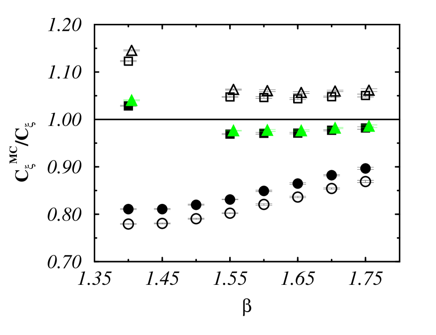
FIG. 2.: The ratio between non-perturbative constants $C^{\rm MC}_{\xi}/C_{\xi}$ for the $O(3)$ model with Symanzik action. Circles (squares, triangles) stand for standard scheme ($E_{1}^{S}$-scheme, $E_{2}^{S}$-scheme). Open (full) symbols mean 2-loop (3-loop) data. The data for the $E_{2}^{S}$-scheme have been slightly shifted horizontally to render the figure clearer.

A The $O(3)$ model with Symanzik action

From the data for $\xi^{(2)}$ and eq. (13) we can compute the constant $C_{\xi}$. We shall call $C^{\rm MC}_{\xi}$ such constant obtained from the Monte Carlo data. If $PT$ is correct and asymptotic scaling holds, this number should be independent of $\beta$ and equal to the prediction of eq. (14) for $n$=3. Therefore the ratio $C^{\rm MC}_{\xi}/C_{\xi}$ should be 1. In Figure 2 we show such ratio as a function of $\beta$ by using eq. (13) at 2-loop and 3-loop [11] for both the standard and energy schemes. We used two different energy schemes defined by the operators $E_{1}^{S}$ and $E_{2}^{S}$, (eqs. (56,57) of the appendix). The respective $\beta_{E}$ are

$$\beta_{E1}\equiv{{w_{1}^{S1}}\over{15/12-E_{1}^{S}}},\qquad\qquad\beta_{E2}\equiv{{w_{1}^{S2}}\over{1-E_{2}^{S}}}.$$ (23)

The perturbative expansions of $E_{1}^{S}$ and $E_{2}^{S}$ are given in the appendix and the Monte Carlo values for both operators are listed in Table IV.

Table IV

Measured values of the two operators (56) and (57) for the $O(3)$ model with Symanzik action.

 $\beta$  $L$  $10^{-5}\cdot\hbox{stat}$  $E^{S}_{1}$  $E^{S}_{2}$  $1.40$  $300$  $4$  $0.840997(3)$  $0.661762(2)$  $1.55$  $340$  $4$  $0.890991(2)$  $0.703158(1)$  $1.60$  $450$  $4$  $0.904603(1)$  $0.714419(1)$  $1.65$  $600$  $4$  $0.917106(1)$  $0.724757(1)$  $1.70$  $800$  $4$  $0.928573(1)$  $0.734231(1)$  $1.75$  $1050$  $0.36$  $0.93917(2)$  $0.74299(1)$  $5.0$  $100$  $7$  $1.14782(2)$  $0.91534(4)$  $10.0$  $100$  $7$  $1.19949(2)$  $0.95812(4)$  $15.0$  $100$  $4$  $1.21650(3)$  $0.97222(2)$

Figure 2 displays an asymptotic approach to unity for increasing $\beta$. The data in the standard scheme (circles) differ from unity by $\sim 15\%$. This is in accordance with previous numerical calculations of $C_{\xi}$ with the tree-level Symanzik action [5]. However, the lack of asymptotic scaling in the energy schemes (squares and triangles) amounts only to $2-3\%$ at 3 loops. Notice also that the two energy schemes agree fairly well; this fact supports the reliability of these schemes. This agreement improves as $\beta$ increases. In the previous section we saw that the systematic error in the corrective factor $C_{\xi^{(2)}}/C_{\xi^{\rm exp}}$ was of the order of 1 per mille which is negligible in Figure 2.

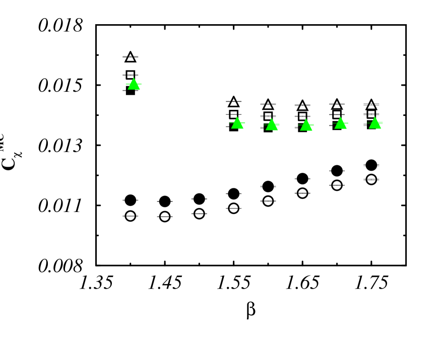
FIG. 3.: The non-perturbative constant $C^{\rm MC}_{\chi}$ for the $O(3)$ model with Symanzik action. The constant is given in units of $\Lambda_{\rm standard}$. Circles (squares, triangles) stand for standard scheme ($E_{1}^{S}$-scheme, $E_{2}^{S}$-scheme). Open (full) symbols mean 2-loop (3-loop) data. The data for the $E_{2}^{S}$-scheme at 3-loop has been slightly shifted horizontally to render the figure clearer.

FIG. 4.: The $PT$ ratio (20) for the for the $O(3)$ model with Symanzik action. Open circles (full circles, open diamonds) stand for the 1-loop (2-loop, 3-loop) result in the standard scheme. Open squares (open up-triangles, open down-triangles) stand for the 1-loop (2-loop, 3-loop) result in the $E_{1}^{S}$-scheme. Full squares (full up-triangles, full down-triangles) stand for the 1-loop (2-loop, 3-loop) result in the $E_{2}^{S}$-scheme. Some data have been slightly shifted horizontally to render the figure clearer.

In Figure 3 we show the constant $C_{\chi}$ computed from our Monte Carlo data at 2 and 3 loops in the standard and energy schemes. At present there are no available exact predictions for this constant. The $1/n^{2}$ calculation [24] provides 0.0625 for the tree-level Symanzik action. After rescaling with (15) this number becomes 0.0127. From the 3-loop data in the energy scheme of Figure 3 one can infer the estimate $C^{\rm MC}_{\chi}=0.0138(2)$ which differs by $\sim 8\%$ from the large-$n$ calculation. This result can be compared with the estimate of ref. [36] which is 0.0146(11); we see that both agree within errors (notice that at 2 loops our result would be 0.0145(3); this error includes the imprecision among the $E^{S}_{1}$ and $E^{S}_{2}$ data). The estimate of ref. [36] has been obtained by using finite-size scaling techniques [37, 38].

We observe that the $1/n$-expansion up to order ${\cal O}(1/n^{2})$ converges well, hence we expect a better agreement if further corrections were added. Finally, notice that the two energy schemes agree much better at 3-loop than at 2-loop.

The results for the $PT$ ratio are reported in Figure 4 up to 3 loops. The data in the standard scheme are far from constant although, as is known for the Symanzik-improved actions [4], the slope is less steep than for the standard action case [28]. The data for the two energy schemes at 2 and 3-loop agree completely. Moreover these data are flatter indicating that scaling has possibly set in. Assuming this onset of scaling, we derive from the data at 2 and 3 loops in these effective schemes $\ln(C_{\chi}/C_{\xi}^{2})=4.54(2)$. Using the prediction (14) $C_{\xi}=0.01249$, we obtain $C_{\chi}=0.0146(2)$ in good agreement with the value inferred from Figure 3. To show the result at 3-loop, the corresponding coefficient of the gamma function for the tree-level Symanzik action has been used. This coefficient can be obtained from [11] after correcting a misprint in their eq. (25): the $(2\pi)^{4}$ dividing the last term in $Z_{1}$ must be instead $(2\pi)^{2}$. We thank M. Falcioni for correspondence about this point, [39]. The 3-loop coefficient is thus

$$\gamma_{2}^{\rm Symanzik}={1\over{(2\pi)^{3}}}\left(-2.01+1.65\;n+0.362\;n^{2}\right)$$ (24)

FIG. 5.: The $KT$ ratio (22) for the $O(3)$ model with Symanzik action.

Now we want to test the $KT$ formulae (21) and (22). A best fit of the data for $\xi$ to eq. (21) is rather unstable. This can be understood as follows: assuming that the $KT$ transition point $\beta_{KT}$ does exist and it is far away, we can expand eq. (21) in powers of $\beta/\beta_{KT}$ obtaining

$$\xi\approx A\exp\left(B\over\sqrt{\beta_{KT}}\right)\exp\left({B\beta}\over{2\beta_{KT}^{3/2}}\right)\equiv A^{\prime}\exp\left(B^{\prime}\beta\right).$$ (25)

This equation shows that actually we are fitting the combination $B^{\prime}\equiv B/(2\beta_{KT}^{3/2})$, therefore the best fit cannot yield reliable information about the precise value of $\beta_{KT}$. However, the fact that the previous analysis within $PT$ gave rather acceptable results indicates that the linear approximation in eq. (25) is good and indeed $\beta_{KT}$ is much larger than our working $\beta$’s.

In Figure 5 the results for the $KT$ ratio (22) are shown. By using the previous conclusion about the large value of $\beta_{KT}$, we have assumed that inside the narrow interval $1.4<\beta<1.75$ the factor $\tau^{r}$ in (22) is almost constant. As a consequence we did not consider it. In ref. [28] this ratio, calculated for the standard action, looked almost constant with the critical exponent $\eta=1/4$. We emphasize that our data have smaller error-bars and so the interval in the vertical axis is almost 7 times finer for our data. This fact allows us to see that our result is clearly not constant. We have estimated the probability $Q$ that the data in Figure 5 follow a straight line. $Q$ is obtained from the tail of the $\chi^{2}$ probability distribution, (we have assumed a gaussian distribution for the point ordinates). We have obtained less than $Q=0.01$ which means that with probability $\sim 99\%$ the data do not follow a straight line. We have repeated the same analysis after removing the first two points (one can argue that they are still far from the scaling region of the $KT$ transition). In this case $Q=0.09$ which still indicates that the data do not lie on a straight line with probability 91%. If the constancy of this ratio was to be a true physical effect then our data for the Symanzik-improved action should stay also constant.

A similar probability calculation shows that also the 2 and 3-loop data in the energy scheme of Figure 4 do not follow a straight line (although the 1-loop data in this scheme is essentially flat). We remark, however, that the effective schemes and the loop corrections have flattened out the data in the $PT$ ratio. In contrast, the increase of the resolution in the statistics has revealed that the $KT$ ratio is not as flat as claimed in ref. [28].

Our results for the $O(3)$ model in the standard scheme do not confirm either of the two scenarios. The lack of asymptotic scaling agrees with previous works using the same Symanzik improved action, [5]. However, in the energy schemes these data present asymptotic scaling at 3 loops within $2-3\%$ for the correlation length as well as an estimate for the magnetic susceptibility that is in reasonable accordance with previous numerical simulations [36] and the $1/n$ expansion. The $PT$ ratio in the energy scheme shows a much flatter behaviour than in the standard scheme. Moreover the agreement between the two energy schemes is a reassuring result.

On the other hand, in the $KT$ scenario, we have seen that the scaling law (22) is badly satisfied. This is in constrast with the data of [28] for the standard action.

B The $O(3)$ model with standard action

In Table V we show the Monte Carlo results for the $O(3)$ model with standard action taken from ref. [6] and the Monte Carlo energy, (see eq. (28) of the appendix), from ref. [40]. The correlation length data corresponds to the exponential definition in eq. (9), so there is no correction factor in this case.

Table V

Data for the $O(3)$ model with standard action. The $\chi$ and $\xi^{\rm exp}$ data has been taken from [6]; the energy data from [40].

 $\beta$  $L\;(\hbox{for $\chi$, $\xi^{\rm exp}$})$  $\chi$  $\xi^{\rm exp}$  $L\;(\hbox{for $E$})$  $E$  $1.50$  $256$  $176.4(2)$  $11.05(1)$  $128$  $0.601597(16)$  $1.60$  $256$  $448.4(7)$  $19.00(2)$  $128$  $0.635722(10)$  $1.70$  $512$  $1263.7(3.3)$  $34.44(6)$  $256$  $0.664240(5)$  $1.75$  $768$  $2197.(15.)$  $47.2(2)$  $256$  $0.676629(4)$  $1.80$  $768$  $3823.(21.)$  $64.5(5)$  $256$  $0.687953(3)$  $1.85$  $768$  $6732.(25.)$  $88.7(5)$  $256$  $0.698351(3)$  $1.90$  $1024$  $11867.(62.)$  $122.7(1.1)$  $256$  $0.707952(3)$  $1.95$  $1024$  $20640.(310.)$  $164.8(5.3)$  $128$  $0.716928(9)$

The asymptotic scaling analysis for these data was done up to 3 loops in [6] while the test for the $KT$ scenario was done in [28]. Here we want to make use of our new perturbative results for the energy up to 4 loops, (eq. (54) of the appendix), and the results of [21] to test asymptotic scaling in the energy scheme for the magnetic susceptibility, the correlation length and the $PT$ ratio. The energy scheme is defined as

$$\beta_{E}\equiv{w_{1}\over{1-E}}.$$ (26)

In Figure 6 we show the ratio $C^{\rm MC}_{\xi}/C_{\xi}$. The lack of asymptotic scaling in the standard schemes is apparent and the energy scheme does not improve it as dramatically as for the Symanzik action. We see that the 4-loop correction in the energy scheme is almost negligible and as a result the departure from asymptotic scaling at 3-loop observed in [6] is still present at 4-loop. The lack of asymptotic scaling in this figure is $\sim 10\%$ for the energy scheme and $15-20\%$ for the standard one.

Figure 7 displays the non-perturbative constant $C_{\chi}$ as computed from the Monte Carlo data. The data in the energy scheme converge around $C_{\chi}=0.0130(5)$ while the $1/n^{2}$ prediction [24] is 0.0127 and the result of [36] was 0.0146(11). The result with our data for the Symanzik action was 0.0138(2). The several Monte Carlo results are compatible with each other suggesting that the truncation error of the series at order $1/n^{2}$ amounts to $\sim 8\%$ when $n=3$.

FIG. 6.: The ratio between non-perturbative constants $C^{\rm MC}_{\xi}/C_{\xi}$ for the $O(3)$ model with standard action. Monte Carlo data from [6]. Open circles (full circles, open diamonds) correspond to 2-loop (3-loop, 4-loop) in the standard scheme; open squares (full squares, open triangles) correspond to the 2-loop (3-loop, 4-loop) in the energy scheme. Some data have been slightly shifted horizontally to render the figure clearer.

FIG. 7.: The non-perturbative constant $C^{\rm MC}_{\chi}$ for the $O(3)$ model with standard action. Monte Carlo data from [6]. Open circles (full circles, open diamonds) correspond to 2-loop (3-loop, 4-loop) in the standard scheme; open squares (full squares, open triangles) correspond to the 2-loop (3-loop, 4-loop) in the energy scheme. Some data have been slightly shifted horizontally to render the figure clearer.

FIG. 8.: The $PT$ ratio for the $O(3)$ model with standard action. Monte Carlo data from [6]. Open circles (full circles, open diamonds, full diamonds) correspond to 1-loop (further corrections) in the standard scheme; open squares (full squares, open triangles, full triangles) correspond to the 1-loop (further corrections) in the energy scheme. Some data have been slightly shifted horizontally to render the figure clearer.

Finally we show the $PT$ ratio up to 4 loops for the standard and energy schemes in Figure 8. The data for the standard scheme is clearly not constant as already seen in [28]. However again the data in the energy scheme is particularly good and stable and allows the determination $\ln(C_{\chi}/C_{\xi}^{2})=4.57(2)$ in excellent agreement with the previous determination by using our data for the Symanzik action (as it should this ratio is independent of the regularization used).

Our results for the $PT$ ratio and the magnetic susceptibility are 4.57(2) and 0.0130(5) respectively. These results, obtained by using the standard action, agree with the previous ones extracted with the Symanzik action. Besides, the ${\cal O}(1/n^{2})$ estimate of $C_{\chi}$ [24] is in good accordance with our data. The deviation from $C_{\xi}$ and the exact result [9] is still of the order $10\%$ even after the inclusion of the 4-loop correction in the energy scheme.

C The $O(8)$ model with standard action

Our Monte Carlo data for the $O(8)$ model is shown in Table II. Our data agree with ref. [7] for the two values of $\beta$ that we have in common. In Table VI we give the energy data taken from [40]. The perturbative expansion for the energy is reported in eq. (55) of the appendix.

FIG. 9.: The ratio $C^{\rm MC}_{\xi}/C_{\xi}$ for the $O(8)$ model with standard action. Open circles (full circles, open diamonds) stand for the 2-loop (3-loop, 4-loop) approximation in the standard scheme. Open squares (full squares, open triangles) stand for the 2-loop (3-loop, 4-loop) approximation in the energy scheme.

In Figure 9 we show for the $O(8)$ model the equivalent of Figure 2. The data converge towards 1 in both the standard and energy schemes. The 4-loop energy scheme for the ratio $C^{\rm MC}_{\xi}/C_{\xi}$ yields 1 up to $\sim 0.5\%$.

Table VI

Energy data for the $O(8)$ model (from ref. [40]).

 $\beta$  $L$  $E$  $4.6$  $128$  $0.603836(9)$  $4.8$  $64$  $0.620987(10)$  $4.9$  $128$  $0.629018(9)$  $5.0$  $64$  $0.636812(10)$  $5.4$  $64$  $0.664983(9)$  $5.8$  $256$  $0.688885(3)$  $6.1$  $256$  $0.704805(3)$  $6.4$  $256$  $0.719168(2)$

The figure clearly displays that the data approach 1 monotonically as the number of loops increases. An important issue then is to understand how big the successive corrections are. At leading order in $1/n$ the coefficients $a_{k}$ in eq. (13) have been computed up to $k$=8 [21]. Comparing with the exactly known coefficients $a_{1}$ and $a_{2}$ we see that the large-$n$ approximations $a_{1,2}(n=8)$ are correct up to 90% and 60% respectively [21, 36]. Assuming a corrective factor $f_{k}=1-2$ such that $a_{k}=f_{k}\cdot a_{k}(n=8)$ for all $k$, then one can see that the next corrections are small and that the convergence towards 1 in Figure 9 is meaningful.

Figure 10 displays the magnetic susceptibility constant as extracted from the Monte Carlo data, $C_{\chi}^{\rm MC}$. We do not show the data in the energy scheme at 2 loops as they are very big $(\sim 0.108)$ and would expand too much the vertical scale of the figure. Data tend to converge around the value $C_{\chi}\approx 0.102$. Taking the results at 4-loop in the energy schemes we obtain $C_{\chi}=0.1028(2)$. The large-$n$ prediction is 0.0915 (up to ${\cal O}(1/n)$, [23]) and 0.103 (up to ${\cal O}(1/n^{2})$, [24]). This ${\cal O}(1/n^{2})$ estimate agrees with our result within $\lesssim 0.5\%$ which is the same amount of deviation from unity seen in Figure 9 for the correlation length. Therefore the $1/n$ expansion agrees fairly well with our data. Notice that data in the standard scheme do not converge monotonically; indeed we have the sequence “2-loop” $>$ “4-loop” $>$ “3-loop”. This is due to the fact that the coefficients $b_{1}$ and $b_{2}$ in eq. (13) have opposite signs.

FIG. 10.: The non-perturbative constant $C_{\chi}$ as extracted from the Monte Carlo data for the $O(8)$ model with standard action. Open circles (full circles, open diamonds) stand for the 2-loop (3-loop, 4-loop) approximation in the standard scheme. Full squares (open triangles) stand for the 3-loop (4-loop) approximation in the energy scheme.

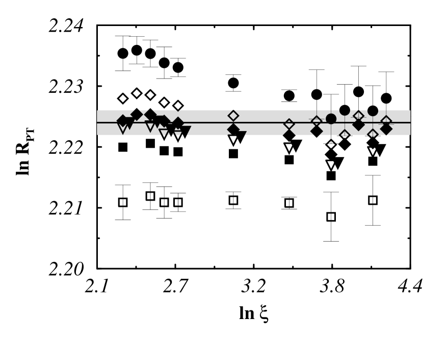
FIG. 11.: The $PT$ ratio for the $O(8)$ model with standard action. Full circles (open diamonds, full diamonds) stand for the 2-loop (further loops) approximation in the standard scheme. Open squares (full squares, open triangles, full triangles) stand for the 1-loop (further loops) approximation in the energy scheme. The highest order corrections in the energy scheme have been slightly shifted horizontally to render the figure clearer.

In Figure 11 we show the $PT$ ratio for the $O(8)$ model. We show this ratio up to 4 loops. We do not show the data at 1 loop in the standard scheme because again they lie far from the window shown in the vertical axis. We have also omitted the error bars in the further corrections to render the figure clearer. The data stabilize for large enough $\ln\xi$ after having included the non-universal corrections. The convergence is extremely good. The straight horizontal line is the prediction (and error) eq. (20) taking the value of eq. (14) for $C_{\xi}$ and the result 0.1028(2) for $C_{\chi}$ from the previous figure. Our data gives $R_{PT}=2.220(5)$.

FIG. 12.: The $KT$ ratio for the $O(8)$ model with standard action. The open circles are the data from our Monte Carlo simulation. The solid line is the prediction of perturbation theory at 4 loops.

Finally Figure 12 shows the $KT$ ratio for the $O(8)$ model. As in the $O(3)$ case, we have neglected the variation of $\tau^{r}$ inside the interval $4.6<\beta<6.5$. The solid line is the $PT$ prediction for this ratio using eq. (13) up to 4 loops, eq. (14) for $C_{\xi}$ and the result from Figure 10 for $C_{\chi}$. We observe that the $KT$ ratio is not constant and that its non-constancy is well explained by $PT$. Notice that the same set of values for $C_{\chi}$ and $C_{\xi}$ explain well both the $PT$ and $KT$ ratios.

In conclusion, $PT$ works fairly well for the $O(8)$ model. The data agree with the exact mass-gap [10] with a precision about 0.5%. Analogously the $1/n^{2}$ prediction for the magnetic susceptibility is in fair accordance with our data within the same error. Moreover the $PT$ and $KT$ ratios are well described by the $PT$ formulae (13).

V Conclusions

We have done a Monte Carlo simulation for the $O(3)$ and $O(8)$ non-linear $\sigma$-models in 2 dimensions. The simulation was performed with the tree-level Symanzik action for the $O(3)$ model and the standard action for the $O(8)$ model. We have improved the statistics with respect to previous works and have taken advantage of the recently calculated 4-loop corrections to scaling [21]. We have taken into account the systematic errors coming from the finite lattice size [20] and from the different non-perturbative constants for the correlation length [21]. In order to reduce them we made use of the correlation length data for the $\xi^{(2)}$ definition, eq. (9), and calculated numerically the corrective factor to pass from $C_{\xi^{\rm exp}}$, eq. (14), to $C_{\xi^{(2)}}$. The result for this numerically calculated factor was in good agreement with the $1/n$ estimate (16).

The ensemble of independent configurations was created with the fast Wolff algorithm, [12]. The independence of the measurements done on these configurations was explicitly verified. However, in the small physical size regime, $\rho=L/\xi\ll 1$ we discovered a worsening in the performance of this algorithm. We argued that this fact can be explained by the presence of large Fortuin-Kasteleyn clusters [33, 34] when $\rho\ll 1$, see Table III.

We have also made use of the data of ref. [6] for the $O(3)$ model with standard action.

In all cases we tested the perturbation theory predictions in both the standard scheme (expansions in the bare coupling $1/\beta$) and the energy scheme (energy modified coupling $1/\beta_{E}$). For this purpose in the appendix we have computed the weak coupling expansion of the energy up to 4 loops for the standard action and 3 loops for the Symanzik action. The fourth loop term in the standard action and the whole expansion up to 3 loops in the Symanzik action are new results of the present paper. Moreover, for the Symanzik action, we computed two different operators, $E^{S}_{1}$ and $E^{S}_{2}$, in order to check the validity of the energy scheme: they should give almost identical results. This check was successful (see figures 2-4).

We saw that the results for the $O(3)$ model agree fairly well with $PT$ in the energy scheme. The $PT$ ratio leads to an almost constant already at 2 loops for both standard and Symanzik actions. This constant was $\ln(C_{\chi}/C_{\xi}^{2})=4.54(2)$ and 4.57(2) for the standard and Symanzik actions respectively. The value observed for the non-perturbative constant $C_{\xi}$ differs from the prediction (14) by almost $2-3\%$ in the Symanzik action and $\gtrsim 10\%$ for the standard one. In both cases we refer to the results in the energy scheme. Even though these differences are still too large, they are much smaller than when obtained from the expansion in the standard $1/\beta$ ($\sim 20\%$). The numbers for the constant $C_{\chi}$ are 0.0138(2) and 0.0130(5) for the Symanzik and standard actions respectively (both in units of $\Lambda_{\rm standard}$). The $1/n^{2}$ prediction [24] is 0.0127. Besides, our determinations are in acceptable accordance with the prediction [41, 42] $C_{\chi}\approx 0.0145$. This number has been extracted from the non-perturbative constant $\lambda_{1}$ obtained in [41] and the ratio between the on-shell and zero-momentum field-renormalization constants $q\equiv Z^{\rm zero-mom}/Z^{\rm on-shell}$ at large $\beta$. This ratio is known in the $1/n$ expansion [42] to be $q=1+0.0132/n+\cdots$. We have computed this ratio from our Monte Carlo data, $Z^{\rm zero-mom}$ being $\chi/\xi^{(2)}$ and $Z^{\rm on-shell}$ being the constant in front of the wall-wall correlation function for large separation $t$

$${\bar{G}}(t)\approx Z^{\rm on-shell}{{\exp\left(L/(2\xi^{\rm exp})\right)}\over{L/\xi^{\rm exp}}}\cosh\left((t-L/2)/\xi^{\rm exp}\right).$$ (27)

The value for $Z^{\rm on-shell}$ presented a plateau as a function of $t$ in the interval $\xi^{\rm exp}/2\lesssim t\lesssim 3\xi^{\rm exp}/2$ and we chose the value at $t=\xi^{\rm exp}$. In Table VII we give our numerical result for the ratio $q$ from our data for the O(3) model with Symanzik action as a function of $\beta$. The average is $q=1.0035(18)$ which is in excellent agreement with the $1/n$ expansion. The fact that $q$ is close to 1 up to few per cent, implies that the estimate $C_{\chi}\approx 0.0145$ is valid within few per cent. We see again a good performance of the $1/n$ expansion even at $n=3$. In particular there is a considerable improvement from the ${\cal O}(1/n)$ approximation [23] in eq. (17) to the ${\cal O}(1/n^{2})$ order [24] in eq. (19). This fact makes us to suspect that also in eq. (16) the ${\cal O}(1/n^{2})$ term would notably improve the agreement with our numerical result for that ratio.

Table VII

Results for the ratio $q$ as a function of $\beta$.

 $\beta$  $1.40$  $1.45$  $1.50$  $1.55$  $1.60$  $1.65$  $1.70$  $q$  $1.0052(40)$  $1.0056(41)$  $1.0028(46)$  $1.0031(34)$  $1.0007(89)$  $1.0043(79)$  $0.9981(60)$

Recall that the Symanzik action has been designed to reduce lattice artifacts [43]. However this improvement can be overwhelmed by the large corrections to asymptotic scaling. The effective schemes can cure this last problem. Hence the combination of an improved action together with the use of an effective scheme should provide the best results. This may be the reason for the good agreement between the $PT$ predictions and our data from the $O(3)$ model with Symanzik action within the energy schemes.

Our analysis of the Monte Carlo results for the $O(8)$ model reveals a satisfactory agreement between the $PT$ predictions and the data. The value (14) for $C_{\xi}$ is recovered within 0.5% and the ${\cal O}(1/n^{2})$ prediction for $C_{\chi}$ agrees within less than 0.5% with our result $0.1028(2)$, (again there is a remarkable improvement between the ${\cal O}(1/n)$ and ${\cal O}(1/n^{2})$ calculations). Analogously the $PT$ ratio tends to stabilize at $\ln(C_{\chi}/C_{\xi}^{2})=2.220(5)$; the same prediction calculated from the previous value for $C_{\chi}$ and the exact $C_{\xi}$ (14) is shown in Figure 11 as an horizontal line at $\ln R_{PT}=2.224(2)$.

We have also checked the set of predictions of the $KT$ scenario for the $O(3)$ model with Symanzik action and the $O(8)$ model with standard action. Figures 5 and 12 show the results for these two cases for the $KT$ ratio. None of them yield a constant as it happened for the data of ref. [28]. We stress the fact that our data have better resolution as the error bars are almost one order of magnitude shorter than in [28]. As for the $O(3)$ model, we showed that the probability of having a straight line after eliminating the first two data points in Figure 5 is less than 10%. The situation for the $O(8)$ model is much clearer: the data are definitively far from constant. In this case perturbation theory predicts fairly well the trend of the data, mainly for the largest correlations. It is worth noticing that the two ratios, $R_{KT}$ and $R_{PT}$, are well explained with the same set of parameters $C_{\xi}$ and $C_{\chi}$ obtained from our analysis. We could not draw a similar $PT$ prediction for the $R_{KT}$ ratio for the $O(3)$ model like the solid line in Figure 12 because the results for $C_{\chi}$ and $C_{\xi}$ for the $O(3)$ model had less precision and the $KT$ ratio is rather sensitive to the precision.

We also tried a fit of the data for the correlation length to the $KT$ law (21). The fit is unstable because the actual value for $\beta_{KT}$ (if it is finite) is much larger than our working $\beta$’s

In summary, $PT$ works well if one includes also the non-universal corrections. Only the correlation length data for the $O(3)$ model with standard action still stays far from the (14) prediction, although these non-universal corrections improve the accordance by a factor of 2. In this respect, we have seen that the energy scheme [18] performs very well and it is a reliable scheme as explicitly proved by using two different operators with the Symanzik data for $O(3)$. In ref. [44] the authors calculate the non-universal corrections to scaling for the spherical model, discovering that they are absent for the energy scheme. We have seen that this good behaviour is almost preserved at low values of $n$.

VI Acknowledgements

We thank Andrea Pelissetto for many useful and stimulating conversations and for a critical reading of the manuscript and Paolo Rossi for a clarification about ref. [41]. B.A. also thanks Wolfhard Janke for a useful comment and Massimo Falcioni for correspondence about ref. [11]. B.A. acknowledges financial support from an INFN contract.

VII Electronic Memorandum

A progress report of the present work was sent to the Lattice-96 proceedings, [45]. While this progress report circulated as an hep-lat preprint, a comment [46] appeared which motivated our reply [47].

VIII Appendix

In this appendix we sketch the calculation of the energy up to 4 loops for the standard action and 3 loops for the tree-level improved Symanzik action.

A Standard action

We define the energy for the standard action as (not summed on $\mu$!)

$$E\equiv\langle{\vec{\phi}(0)}\cdot{\vec{\phi}(0+{\hat{\mu}})}\rangle$$ (28)

which in the weak coupling expansion can be written as

$$E(\beta)=1-{w_{1}\over\beta}-{w_{2}\over\beta^{2}}-{w_{3}\over\beta^{3}}-{w_{4}\over\beta^{4}}-\cdots$$ (29)

The first two coefficients $w_{1}$ and $w_{2}$ can be straightforwardly computed giving

$$w_{1}={{\left(n-1\right)}\over 4},\qquad\qquad\qquad w_{2}={{\left(n-1\right)}\over 32}.$$ (30)

FIG. 13.: Feynman diagrams contributing to the 3-loop coefficient of the free energy. Crosses stand for insertions of the measure lagrangian that comes from the Dirac delta in eq. (32).

The order ${\cal O}(1/\beta^{3})$ coefficient has been computed in [44] (for the $O(3)$ model it was also calculated in [48] and for general $n$ in [49]). We have checked their result by computing the diagrams for the free energy in Figure 13 and by making use of the relationship

$$E = {1\over{2\,V}}{{\partial}\over{\partial\beta}}\ln Z,$$ (31)

$$Z \equiv \int\,{\cal D}{\vec{\phi}}(x)\,\delta({\vec{\phi}}(x)^{2}-1)\,\exp\left({-S^{\rm standard}}\right).$$ (32)

$V$ is the space-time volume and ${\cal D}$ the standard functional measure. In the evaluation of the Feynman diagrams the following identity is useful

$${\widehat{\left(p_{1}+p_{2}\right)}}^{2} + {\widehat{\left(p_{1}+p_{3}\right)}}^{2}+{\widehat{\left(p_{1}+p_{4}\right)}}^{2}={\hat{p}_{1}}^{2}+{\hat{p}_{2}}^{2}+{\hat{p}_{3}}^{2}+{\hat{p}_{4}}^{2}-\Sigma_{1234},$$ (34)

$$\Sigma_{ijkl}\equiv\sum_{\mu}{\hat{p}_{i\mu}}{\hat{p}_{j\mu}}{\hat{p}_{k\mu}}{\hat{p}_{l\mu}},$$

provided that $p_{1}+p_{2}+p_{3}+p_{4}=0\;$ [44]. We make use of the standard notation, ${\hat{p}}_{\mu}\equiv 2\sin(p_{\mu}/2)$ and ${\hat{p}}^{2}\equiv\sum_{\mu}{\hat{p}}_{\mu}^{2}$. Another relation useful during the evaluation of tadpole diagrams is

$${\widehat{\left(p_{1}+p_{2}\right)}}^{2}={\hat{p}_{1}}^{2}+{\hat{p}_{2}}^{2}-{1\over 4}\,{\hat{p}_{1}}^{2}\,{\hat{p}_{2}}^{2}+\hbox{odd terms},$$ (35)

valid for any pair of momenta $p_{1}$ and $p_{2}$.

The result for $w_{3}$ is

$$w_{3}={{\left(n-1\right)^{2}}\over 16}\,K+{{\left(n-1\right)}\over 16}\,\left({1\over 6}-K+{1\over 3}J\right).$$ (36)

$K$ and $J$ are finite integrals

$$K \equiv \int^{+\pi}_{-\pi}{\rm D}_{3}\;{{\Delta_{12}\Delta_{34}}\over{{\hat{p}_{1}}^{2}\;{\hat{p}_{2}}^{2}\;{\hat{p}_{3}}^{2}\;{\hat{p}_{4}}^{2}}}=0.0958876$$ (37)

$$J \equiv \int^{+\pi}_{-\pi}{\rm D}_{3}\;{{\left(\Sigma_{1234}\right)^{2}}\over{{\hat{p}_{1}}^{2}\;{\hat{p}_{2}}^{2}\;{\hat{p}_{3}}^{2}\;{\hat{p}_{4}}^{2}}}=0.136620$$ (38)

where the measure ${\rm D}_{3}$ is

$${\rm D}_{3}\equiv{{{\rm d}^{2}p_{1}}\over{\left(2\pi\right)^{2}}}{{{\rm d}^{2}p_{2}}\over{\left(2\pi\right)^{2}}}{{{\rm d}^{2}p_{3}}\over{\left(2\pi\right)^{2}}}{{{\rm d}^{2}p_{4}}\over{\left(2\pi\right)^{2}}}\left(2\pi\right)^{2}\delta(p_{1}+p_{2}+p_{3}+p_{4})$$ (39)

and

$$\Delta_{ij} \equiv {\widehat{\left(p_{i}+p_{j}\right)}}^{2}-{\hat{p}_{i}}^{2}-{\hat{p}_{j}}^{2},$$ (40)

$$\Delta_{i-j} \equiv {\widehat{\left(p_{i}-p_{j}\right)}}^{2}-{\hat{p}_{i}}^{2}-{\hat{p}_{j}}^{2},$$ (41)

$\Delta_{i-j}$ will be used later.

FIG. 14.: Feynman diagrams contributing to the 4-loop coefficient of the free energy. Same meaning as in Figure 9 for the crosses.

In Figure 14 we show the diagrams needed for the evaluation of $w_{4}$. Again eqs. (34) and (35) are useful. No new identities among momenta are needed. The result is

$$w_{4} = {{3\left(n-1\right)}\over 8}\left({1\over 128}-{1\over 2}H_{1}-{1\over 4}H_{2}-{1\over 3}H_{3}+{1\over 24}J-{1\over 8}K-{1\over 4}H_{5}\right)+$$ (44)

$${{3\left(n-1\right)^{2}}\over 8}\left({1\over 256}+{1\over 2}H_{1}+{1\over 4}H_{2}+{1\over 3}H_{3}+{1\over 12}H_{4}+{1\over 8}K+{1\over 3}H_{5}\right)-$$

$${{\left(n-1\right)^{3}}\over 32}H_{5}.$$

$K$ and $J$ are given in eq. (38) while $H_{1}$, …, $H_{5}$ are genuine 4-loop integrals

$$H_{1} \equiv \int^{+\pi}_{-\pi}{\rm D}_{4}\;{{\Delta_{12}\;\Delta_{34}\;\Sigma_{1256}}\over{{\hat{p}_{1}}^{2}\;{\hat{p}_{2}}^{2}\;{\hat{p}_{3}}^{2}\;{\hat{p}_{4}}^{2}\;{\hat{p}_{5}}^{2}\;{\hat{p}_{6}}^{2}}}=0.0378134$$ (45)

$$H_{2} \equiv \int^{+\pi}_{-\pi}{\rm D}_{4}\;{{\Delta_{34}\;\Sigma_{1234}\;\Sigma_{1256}}\over{{\hat{p}_{1}}^{2}\;{\hat{p}_{2}}^{2}\;{\hat{p}_{3}}^{2}\;{\hat{p}_{4}}^{2}\;{\hat{p}_{5}}^{2}\;{\hat{p}_{6}}^{2}}}=-0.0322778$$ (46)

$$H_{3} \equiv \int^{+\pi}_{-\pi}{\rm D}_{4}\;{{\Delta_{13}\;\Delta_{45}\;\Delta_{2-6}}\over{{\hat{p}_{1}}^{2}\;{\hat{p}_{2}}^{2}\;{\hat{p}_{3}}^{2}\;{\hat{p}_{4}}^{2}\;{\hat{p}_{5}}^{2}\;{\hat{p}_{6}}^{2}}}=-0.0136824$$ (47)

$$H_{4} \equiv \int^{+\pi}_{-\pi}{\rm D}_{4}\;{{\Sigma_{1234}\;\Sigma_{3456}\;\Sigma_{1256}}\over{{\hat{p}_{1}}^{2}\;{\hat{p}_{2}}^{2}\;{\hat{p}_{3}}^{2}\;{\hat{p}_{4}}^{2}\;{\hat{p}_{5}}^{2}\;{\hat{p}_{6}}^{2}}}=0.0411085$$ (48)

$$H_{5} \equiv \int^{+\pi}_{-\pi}{\rm D}_{4}\;{{\Delta_{12}\;\Delta_{34}\;\Delta_{56}}\over{{\hat{p}_{1}}^{2}\;{\hat{p}_{2}}^{2}\;{\hat{p}_{3}}^{2}\;{\hat{p}_{4}}^{2}\;{\hat{p}_{5}}^{2}\;{\hat{p}_{6}}^{2}}}=-0.0501528$$ (49)

The measure for the 4-loop integrals is

$${\rm D}_{4} \equiv {{{\rm d}^{2}p_{1}}\over{\left(2\pi\right)^{2}}}{{{\rm d}^{2}p_{2}}\over{\left(2\pi\right)^{2}}}{{{\rm d}^{2}p_{3}}\over{\left(2\pi\right)^{2}}}{{{\rm d}^{2}p_{4}}\over{\left(2\pi\right)^{2}}}{{{\rm d}^{2}p_{5}}\over{\left(2\pi\right)^{2}}}{{{\rm d}^{2}p_{6}}\over{\left(2\pi\right)^{2}}}\times$$ (51)

$$\qquad\left(2\pi\right)^{2}\delta(p_{1}+p_{2}+p_{3}+p_{4})\left(2\pi\right)^{2}\delta(p_{5}+p_{6}+p_{3}+p_{4}).$$

Numerically at 4 loops the expansion (29) reads

$$E(\beta)= 1 -{{n-1}\over{4\beta}}-{{n-1}\over{32\beta^{2}}}-{{0.00726994\;(n-1)+0.00599298\;(n-1)^{2}}\over\beta^{3}}-$$ (53)

$${{0.00291780\;(n-1)+0.00332878\;(n-1)^{2}+0.00156728\;(n-1)^{3}}\over\beta^{4}}.$$

For $n=3$ and $n=8$ the expansion (53) becomes

$$E(\beta,\,n=3) = 1-{1\over{2\beta}}-{1\over{16\beta^{2}}}-{0.03851\over\beta^{3}}-{0.03169\over\beta^{4}},$$ (54)

$$E(\beta,\,n=8) = 1-{7\over{4\beta}}-{7\over{32\beta^{2}}}-{0.3445\over\beta^{3}}-{0.7211\over\beta^{4}}.$$ (55)

B Symanzik action

As for the Symanzik action, we have used two different local operators to define the so-called energy-scheme (not summed over $\mu$!)

$$E^{S}_{1} \equiv \langle{4\over 3}{\vec{\phi}(0)}\cdot{\vec{\phi}(0+{\hat{\mu}})}-{1\over 12}{\vec{\phi}(0)}\cdot{\vec{\phi}(0+2{\hat{\mu}})}\rangle,$$ (56)

$$E^{S}_{2} \equiv \langle{\vec{\phi}(0)}\cdot{\vec{\phi}(0+{\hat{\mu}})}\rangle.$$ (57)

The first operator is the energy density for the Symanzik-improved action, hence its weak coupling expansion can be computed by evaluating the free energy and making use of eq. (32). In ref. [50] it was computed up to 2 loops for the $n=3$ case. We have checked their result which for any $n$ can be written as

$$E^{S}_{1}(\beta) = {15\over 12}-{w^{S1}_{1}\over\beta}-{w^{S1}_{2}\over\beta^{2}}-{w^{S1}_{3}\over\beta^{3}}-\cdots,$$ (60)

$$w^{S1}_{1}={{\left(n-1\right)}\over 4},$$

$$w^{S1}_{2}={{\left(n-1\right)}\over 48}\;Y_{1}\,\left(1-{5\over 24}Y_{1}\right).$$

$Y_{1}$ is a 1-loop integral. The notation $\Pi_{p}$ will mean the inverse propagator for the Symanzik action

$$\Pi_{p}\equiv{\hat{p}}^{2}+{1\over 12}\Box_{p},\qquad\qquad\qquad\Box_{p}\equiv\sum_{\mu}{\hat{p}}^{4}_{\mu}.$$ (61)

The 1-loop integral is

$$Y_{1}\equiv\int^{+\pi}_{-\pi}{{{\rm d}^{2}p}\over{\left(2\pi\right)^{2}}}\;{{\Box_{p}}\over{\Pi_{p}}}=2.043576$$ (62)

The 3-loop coefficient can be obtained by evaluating a set of diagrams analogous to the one in Figure 13. Useful identities are

$$\Pi_{p+q} + \Pi_{p+k}+\Pi_{p+r}=\Pi_{p}+\Pi_{q}+\Pi_{k}+\Pi_{r}-\Sigma^{S},$$ (64)

$$\Sigma^{S}\equiv{4\over 3}\sum_{\mu}{\hat{p}_{\mu}}{\hat{q}_{\mu}}{\hat{k}_{\mu}}{\hat{r}_{\mu}}-{1\over 12}\sum_{\mu}{\widehat{2p_{\mu}}}{\widehat{2q_{\mu}}}{\widehat{2k_{\mu}}}{\widehat{2r_{\mu}}},$$

valid whenever $p+q+k+r=0$ and

$$\Pi_{p+q}=\Pi_{p}+\Pi_{q}-{1\over 12}\Pi_{p}\Box_{q}-{1\over 12}\Pi_{q}\Box_{p}+{5\over 144}\Box_{p}\Box_{q}+\hbox{odd terms}$$ (65)

for any pair of momenta $p$ and $q$. The result for $w^{S1}_{3}$ is

$$w^{S1}_{3} = {{\left(n-1\right)^{2}}\over 16}K^{S}+{{\left(n-1\right)}\over 2}\Bigg{(}{1\over 24}+{1\over 24}J^{S}-{1\over 8}K^{S}+{1\over 288}Y_{2}-$$ (67)

$$Y_{1}\left({5\over 96}+{5\over 1728}Y_{2}\right)+Y_{1}^{2}\left({11\over 384}+{25\over 41472}Y_{2}\right)-{205\over 41472}Y_{1}^{3}\Bigg{)}.$$

$Y_{2}$ is a 1-loop integral

$$Y_{2}\equiv\int^{+\pi}_{-\pi}{{{\rm d}^{2}p}\over{\left(2\pi\right)^{2}}}\;{{\Box_{p}^{2}}\over{\left(\Pi_{p}\right)^{2}}}=4.783071$$ (68)

The 3-loop integrals are

$$K^{S} \equiv \int^{+\pi}_{-\pi}{\rm D}_{3}\;{{\Delta^{S}_{12}\Delta^{S}_{34}}\over{{\Pi_{p_{1}}}\;{\Pi_{p_{2}}}\;{\Pi_{p_{3}}}\;{\Pi_{p_{4}}}}}=0.0673316$$ (69)

$$J^{S} \equiv \int^{+\pi}_{-\pi}{\rm D}_{3}\;{{\left(\Sigma^{S}\right)^{2}}\over{{\Pi_{p_{1}}}\;{\Pi_{p_{2}}}\;{\Pi_{p_{3}}}\;{\Pi_{p_{4}}}}}=0.104551$$ (70)

where $\Delta^{S}_{12}\equiv\left(\Pi_{p1+p2}-\Pi_{p1}-\Pi_{p2}\right)$.

Numerically $E^{S}_{1}$ is

$$E^{S}_{1}(\beta)= {15\over 12}-{{n-1}\over{4\beta}}-{{0.0244486\;(n-1)}\over{\beta^{2}}}-$$ (72)

$${{0.00449054\;(n-1)+0.00420822\;(n-1)^{2}}\over\beta^{3}}.$$

For $n=3$ it is

$$E^{S}_{1}(\beta,n=3)={15\over 12}-{1\over{2\beta}}-{0.04890\over\beta^{2}}-{0.02581\over\beta^{3}}.$$ (73)

FIG. 15.: Feynman diagrams contributing to the 3-loop coefficient of the operator $E^{S}_{2}$, eq. (57). Crosses and black spots stand for insertions of measure and the operator $E^{S}_{2}$ respectively.

The second operator used is eq. (57). The computation of the coefficients in the weak expansion

$$E^{S}_{2}(\beta)=1-{w^{S2}_{1}\over\beta}-{w^{S2}_{2}\over\beta^{2}}-{w^{S2}_{3}\over\beta^{3}}-\cdots$$ (74)

requires the evaluation of diagrams with an insertion of the operator in (57). In Figure 15 we show the diagrams necessary for the 3-loop coefficient. The results for all coefficients are

$$w^{S2}_{1} = {{\left(n-1\right)}\over 4}\left(1-{1\over 12}Y_{1}\right),$$ (75)

$$w^{S2}_{2} = {{\left(n-1\right)}\over 32}\left(Y_{1}\left({3\over 2}+{5\over 216}Y_{2}\right)-{1\over 18}Y_{2}-{49\over 144}Y_{1}^{2}-1\right)$$ (76)

$$w^{S2}_{3} = {{\left(n-1\right)^{2}}\over 16}\left(2{\overline{K^{S}}}-{\widetilde{K}^{S}}\right)+{{\left(n-1\right)}\over 16}\Bigg{(}{\widetilde{K}^{S}}-2{\overline{K^{S}}}+{2\over 3}{\overline{J^{S}}}-{1\over 3}{\widetilde{J^{S}}}+,$$ (80)

$${13\over 24}-{3529\over 41472}Y_{1}^{3}+{23\over 288}Y_{2}+{5\over 5184}Y_{2}^{2}-{1\over 432}Y_{3}+$$

$$Y_{1}^{2}\left({61\over 128}+{695\over 41472}Y_{2}-{25\over 62208}Y_{3}\right)+$$

$$Y_{1}\left(-{27\over 32}-{127\over 1728}Y_{2}-{25\over 62208}Y_{2}^{2}+{5\over 2592}Y_{3}\right)\Bigg{)}.$$

The integrals are

$$Y_{3} \equiv \int^{+\pi}_{-\pi}{{{\rm d}^{2}p}\over{\left(2\pi\right)^{2}}}\;{{\Box_{p}^{3}}\over{\left(\Pi_{p}\right)^{3}}}=11.816615$$ (81)

$${\widetilde{K^{S}}} \equiv \int^{+\pi}_{-\pi}{\rm D}_{3}\;{{\Delta^{S}_{12}\;\Delta_{34}}\over{{{\Pi_{p_{1}}}\;{\Pi_{p_{2}}}\;{\Pi_{p_{3}}}\;{\Pi_{p_{4}}}}}}=0.0578002$$ (82)

$${\overline{K^{S}}} \equiv \int^{+\pi}_{-\pi}{\rm D}_{3}\;{{\Delta^{S}_{12}\;\Delta^{S}_{34}\;{\hat{p}_{1}}^{2}}\over{\left({\Pi_{p_{1}}}\right)^{2}\;{\Pi_{p_{2}}}\;{\Pi_{p_{3}}}\;{\Pi_{p_{4}}}}}=0.0572726$$ (83)

$${\widetilde{J^{S}}} \equiv \int^{+\pi}_{-\pi}{\rm D}_{3}\;{{\Sigma_{1234}\;\Sigma^{S}}\over{{\Pi_{p_{1}}}\;{\Pi_{p_{2}}}\;{\Pi_{p_{3}}}\;{\Pi_{p_{4}}}}}=0.0809553$$ (84)

$${\overline{J^{S}}} \equiv \int^{+\pi}_{-\pi}{\rm D}_{3}\;{{\Sigma^{S}\;\Sigma^{S}\;{\hat{p}_{1}}^{2}}\over{\left({\Pi_{p_{1}}}\right)^{2}\;{\Pi_{p_{2}}}\;{\Pi_{p_{3}}}\;{\Pi_{p_{4}}}}}=0.0867806$$ (85)

Numerically $E^{S}_{2}$ is

$$E^{S}_{2}(\beta)= 1 -{{0.207425\;(n-1)}\over{\beta}}-{{0.0189010\;(n-1)}\over{\beta^{2}}}-$$ (87)

$${{0.00353381\;(n-1)+0.00354656\;(n-1)^{2}}\over\beta^{3}}.$$

For $n=3$ it is

$$E^{S}_{2}(\beta,n=3)=1-{0.41485\over\beta}-{0.03780\over\beta^{2}}-{0.02125\over\beta^{3}}.$$ (88)

Another method to calculate the previous coefficients has been proposed in [51, 52, 53]. The Monte Carlo determination of any operator at large $\beta$ can be straightforwardly compared to its perturbative expansion, allowing an estimate of the perturbative coefficients. In the last three rows of Table IV we give the values of $E^{S}_{1}$ and $E^{S}_{2}$ for $\beta=5$, 10, 15.

The ${\cal O}(1/\beta)$ coefficient can be obtained comparing the energy at $\beta=15$ with the expression $15/12-w^{S1}_{1}/\beta$ and $1-w^{S2}_{1}/\beta$. We obtain $w^{S1}_{1}=0.502(1)$ and $w^{S2}_{1}=0.4167(3)$.

Assuming that the exact first order coefficient is known, one can use the value of the energy at $\beta=10$ to determine the ${\cal O}(1/\beta^{2})$ coefficient obtaining $w^{S1}_{2}=0.051(2)$ and $w^{S2}_{2}=0.039(4)$.

Similarly, by using the exact two first coefficients and the value at $\beta=5$ one obtains $w^{S1}_{3}=0.028(2)$ and $w^{S2}_{3}=0.022(5)$.

These results are clearly influenced by the next orders and likely also by the small size ($L=100$) of the lattice used to calculate the energies for these large $\beta$’s. A better analysis must use a global fit for all coefficients and higher precision in the Monte Carlo determination of the operator. Here we have used this technique just as an approximate check for our analytical computation.

REFERENCES

- [1] A. M. Polyakov, Phys. Lett. B59 (1975) 79.
- [2] E. Brézin and J. Zinn-Justin, Phys. Rev. B14 (1976) 3110.
- [3] A. A. Belavin and A. M. Polyakov, JETP Lett. 22 (1975) 245.
- [4] B. Berg, S. Meyer and I. Montvay, Nucl. Phys. B235 [FS11] (1984) 149.
- [5] P. Hasenfratz and F. Niedermayer, Nucl. Phys. B337 (1990) 233.
- [6] J. Apostolakis, C. F. Baillie and G. C. Fox, Phys. Rev. D43 (1991) 2687.
- [7] U. Wolff, Phys. Lett. B248 (1990) 335.
- [8] B. Allés and M. Beccaria, Phys. Rev. D52 (1995) 6481.
- [9] P. Hasenfratz, M. Maggiore and F. Niedermayer, Phys. Lett. B245 (1990) 522.
- [10] P. Hasenfratz and F. Niedermayer, Phys. Lett. B245 (1990) 529.
- [11] M. Falcioni and A. Treves, Nucl. Phys. B265 (1986) 671.
- [12] U. Wolff, Phys. Rev. Lett. 62 (1989) 361.
- [13] N. D. Mermin and H. Wagner, Phys. Rev. Lett. 17 (1966) 1133.
- [14] A. Patrascioiu and E. Seiler, J. Stat. Phys. 69 (1992) 573; Nucl. Phys. (Proc. Suppl.) 30 (1993) 184.
- [15] J. M. Kosterlitz and D. J. Thouless, J. Phys. C6 (1973) 1181.
- [16] J. M. Kosterlitz, J. Phys. C7 (1974) 1046.
- [17] K. Symanzik, Nucl. Phys. B226 (1983) 205.
- [18] G. Martinelli, G. Parisi and R. Petronzio, Phys. Lett. B100 (1981) 485.
- [19] M. Lüscher, Commun. Math. Phys. 104 (1986) 177.
- [20] S. Caracciolo and A. Pelissetto, hep-lat/9607013.
- [21] S. Caracciolo and A. Pelissetto, Nucl. Phys. B455 (1995) 619.
- [22] B. Berg, Z. Phys. C20 (1983) 243.
- [23] P. Biscari, M. Campostrini and P. Rossi, Phys. Lett. B242 (1990) 225.
- [24] H. Flyvbjerg and F. Laursen, Phys. Lett. B266 (1991) 99.
- [25] D. J. Amit, Y. Y. Goldschmidt and G. Grinstein, J. Phys. A13 (1980) 585.
- [26] P. Butera and M. Comi, Phys. Rev. B47 (1993) 11969.
- [27] R. Kenna and A. C. Irving, Phys. Lett. B351 (1995) 273; Nucl. Phys. (Proc. Suppl.) B42 (1995) 773.
- [28] A. Patrascioiu and E. Seiler, hep-lat/9508014.
- [29] W. Janke, hep-lat/9609045.
- [30] M. Campostrini, A. Pelissetto, P. Rossi and E. Vicari, hep-lat/9603002.
- [31] A. Buonanno and G. Cella, Phys. Rev. D51 (1995) 5865.
- [32] U. Wolff, Nucl. Phys. B334 (1990) 581.
- [33] C. M. Fortuin and P. W. Kasteleyn, Physica 57 (1972) 536.
- [34] R. Swendsen and J.-S. Wang, Phys. Rev. Lett. 58 (1987) 86.
- [35] S. Meyer, unpublished, quoted in [38].
- [36] S. Caracciolo, R. G. Edwards, T. Mendes, A. Pelissetto and A. D. Sokal, Nucl. Phys. (Proc. Suppl.) B47 (1996) 763.
- [37] J. K. Kim, Phys. Rev. Lett. 70 (1993) 1735.
- [38] S. Caracciolo, R. G. Edwards, A. Pelissetto and A. D. Sokal, Phys. Rev. Lett. 75 (1995) 1891.
- [39] M. Falcioni, private communication.
- [40] T. Mendes, A. Pelissetto and A. D. Sokal, hep-lat/9604015.
- [41] J. Balog and M. Niedermaier, hep-th/9612039.
- [42] M. Campostrini, A. Pelissetto, P. Rossi and E. Vicari, in preparation.
- [43] K. Symanzik, in VI Int. Conf. on Mathematical Physics (1981) pg. 47.
- [44] S. Caracciolo and A. Pelissetto, Nucl. Phys. B420 (1994) 141.
- [45] B. Allés, A. Buonanno and G. Cella, hep-lat/9608002.
- [46] A. Patrascioiu and E. Seiler, hep-lat/9608138.
- [47] B. Allés, A. Buonanno and G. Cella, hep-lat/9609024.
- [48] B. Berg and M. Lüscher, Nucl. Phys. B190 (1981) 412.
- [49] M. Lüscher, unpublished, quoted in [7].
- [50] A. Di Giacomo, F. Farchioni, A. Papa and E. Vicari, Phys. Lett. B276 (1992) 148.
- [51] A. Di Giacomo and E. Vicari, Phys. Lett. B275 (1992) 429.
- [52] B. Allés, M. Campostrini, A. Di Giacomo, Y. Gündüç and E. Vicari, Phys. Rev. D48 (1993) 2284.
- [53] B. Allés, M. Beccaria and F. Farchioni, Phys. Rev. D54 (1996) 1044.