Four-dimensional Simulation of the Hot Electroweak Phase Transition with the SU(2) Gauge-Higgs Model
Abstract
We study the finite-temperature electroweak phase transition of the minimal standard model within the four-dimensional SU(2) gauge-Higgs model. Monte Carlo simulations are performed for intermediate values of the Higgs boson mass in the range GeV on a lattice with the temporal size . The order of the transition is systematically examined using finite-size scaling methods. Behavior of the interface tension and the latent heat for an increasing Higgs boson mass is also investigated. Our results suggest that the first-order transition terminates around GeV.
pacs:
11.10.Wx, 11.15.Ha, 12.15.-yI Introduction
The possibility that the baryon number asymmetry of the universe was generated in the course of the electroweak phase transition in the early universe has been much discussed. One of the conditions necessary for a realization of this possibility is the presence of out-of-equilibrium process during the transition. If the transition is of first order with a sufficient strength, super cooling could occur and the universe could have been driven out of equilibrium. This raises the question whether the electroweak phase transition undergoes a strong enough first-order transition for a realistic Higgs boson mass.
In the minimal standard model the essential features of the finite-temperature electroweak phase transition are expected to be controlled by the SU(2) gauge-Higgs sector. Hence finite-temperature studies of the SU(2) gauge-Higgs model represent a first step in understanding the electroweak transition. In the past two approaches have been taken for a non-perturbative analysis of the transition in this model by means of Monte Carlo simulations (for reviews, see Refs. [1, 2]). One approach is to employ the original four-dimensional model. The other is to treat a three-dimensional model derived by a dimensional reduction of the original model in time. In the three-dimensional approach many studies have been made covering a wide range of the Higgs boson mass GeV [3, 4, 5, 6, 7]. In particular, it has recently been reported that the phase transition is absent for GeV[4, 7]. On the other hand, studies with the four-dimensional model[8, 9, 10, 11, 12] have been less extensive, and systematic analyses have been limited to relatively light Higgs boson masses of GeV[10, 11, 12]. Since the Higgs boson mass is experimentally bounded by GeV[13], it is important to extend the study of the four-dimensional model toward heavier Higgs boson masses.
In this article, we report results of our simulation of the four-dimensional model for the Higgs boson mass in the range GeV. Our aim is a systematic analysis of the strength of the transition, which is known to be of strong first order for light Higgs boson, as the Higgs boson mass increases. For this purpose finite-size scaling analyses of susceptibility and the Binder cumulant are carried out. We also study latent heat and interface tension in order to examine the strength of the transition in terms of physical quantities.
In Sec. II we describe some details of our simulation. Monte Carlo time histories of observables are discussed in Sec. III. Results of finite-size scaling analyses are presented in Sec. IV. In Sec. V and VI we report measurement of latent heat and interface tension. Our results are summarized in Sec. VII. In Appendix we describe our procedure to estimate the Higgs boson mass and the critical temperature for our simulation points from published results.
II Simulation
We employ the standard lattice action given by
| (1) |
where the radial part is defined by the decomposition of the complex matrix Higgs field SU(2). All of our simulations are made for the temporal extent . We set the gauge coupling . Simulations are made for 6 values of the scalar self-coupling , choosing the hopping parameter in the vicinity of the transition point. The parameter values of all of our runs are listed in Table I. Also listed in the table are estimates of the zero-temperature Higgs boson mass and the critical temperature at the transition point of lattice. These estimates are obtained by interpolating available data for and at , , (GeV) [11, 12], (GeV) and [8]. The procedure of the interpolation is described in Appendix.
For each value of runs are made on an lattice with , and in addition with for GeV ). Gauge and scalar fields are updated with a combination of the heat bath[14] and overrelaxation[15] algorithms in the ratio displayed in Table II, which has been reported to have the fastest decorrelation time in terms of number of sweeps in Ref. [11]. We make iterations of the combined updates for each parameter point except for the run with , where we make iterations.
Observables are measured at each iteration. Our analyses are mainly made in terms of the quantities defined by
| (2) | |||||
| (3) | |||||
| (4) |
where is the spatial part of the scalar hopping term in the action, represents the angular part of and the squared Higgs condensate.
III Monte Carlo Time History
A qualitative test for a first-order phase transition is provided by Monte Carlo time histories of observables and their histograms. In Fig. 1 we show the time history of and its histogram for the largest volume for each . For the lightest Higgs boson GeV (Fig. 1(a)), a clear flip-flop behavior is seen, which is reflected in the double peak structure of the histogram of . If we increase the Higgs boson mass, the flip-flop behavior becomes milder, indicating a weakening of the first-order transition. It can be seen, however, up to GeV (Fig. 1(d)). A double peak structure of the histogram also persists up to this value of . These observations provide qualitative indication for a first-order transition up to GeV.
On the other hand, for the heavier Higgs boson of and GeV, we cannot discern a flip-flop behavior nor a double peak structure in the histogram. We have analyzed the histogram varying the hopping parameter around the value of the simulation through the reweighting technique[16]. For GeV (Fig. 1(e)), we found that the histogram changes to a narrow flat peak at , while only a sharp single peak structure has been seen for GeV (Fig. 1(f)). This suggests that a first-order transition is either absent, or extremely weak at these Higgs boson masses.
IV Finite-Size Scaling Analysis
Let us consider the susceptibility of defined by
| (5) |
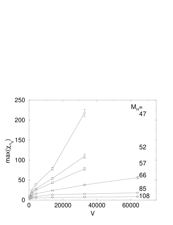
with the spatial volume. On a finite lattice this quantity has a peak at the pseudo critical point . If the transition is of first order, the maximum value of the peak should increase linearly in volume, and the pseudo critical point should converge to the value at infinite volume linearly in [17]. On the other hand, the maximum value should remain constant if there is no phase transition.
We calculate the maximum value and the position of the peak with the standard reweighting technique[16]. Errors are estimated by a jackknife analysis using - sweeps as the bin size, which is chosen from stability of the magnitude of error as a function of bin size and varies with coupling parameters and lattice sizes.
In Fig. 2 results for the maximum value of the susceptibility of is shown as a function of the volume . For GeV the increase of the maximum value is consistent with a linear behavior, quantitatively supporting a first-order transition for this region of Higgs boson mass. In contrast, we observe a very flat volume dependence for GeV, albeit the maximum value is increasing slowly in the range of volume used here.
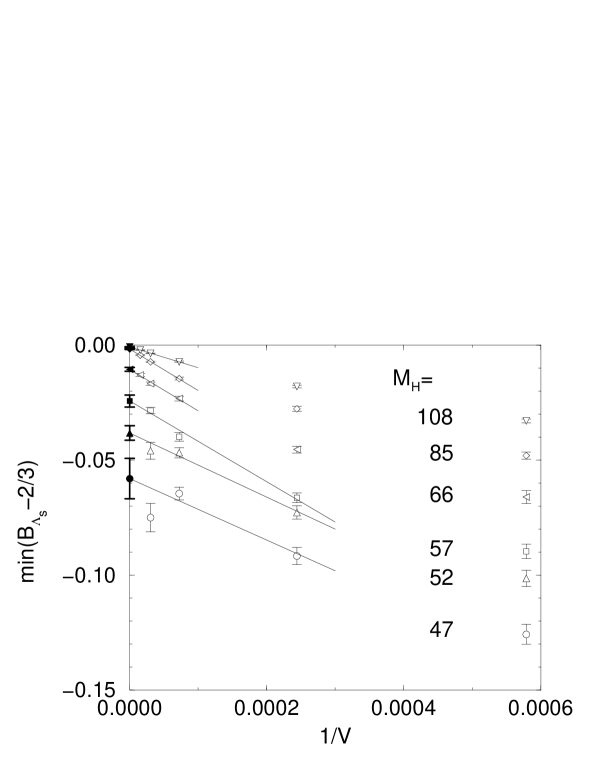
Another useful indicator of a first-order transition is the Binder cumulant defined by
| (6) |
For the case of a first-order phase transition the value of deviates from in the infinite volume limit, while it converges to otherwise.
In Fig. 3 we plot the valley depth of the Binder cumulant of as a function of the inverse volume obtained by a reweighting procedure similar to that for the susceptibility . Lines are linear fits to the largest three volumes for each . For GeV the value extrapolated to the infinite volume clearly deviates from , providing additional evidence for a first-order transition. For GeV the deviation decreases by an order of magnitude, although still finite within the error. In Fig. 4 the deviation of from is plotted as a function of the Higgs boson mass. It can be seen that the strength of the first-order transition rapidly diminishes toward larger .
Our results for the susceptibility and the Binder cumulant clearly show that the transition is of first order for GeV. It is also clear that the transition, if first order, is a very weak one at GeV and 108GeV. It is possible that the transition turns into a crossover for this range of . Data for larger volumes are needed, however, for a conclusive analysis on this point.
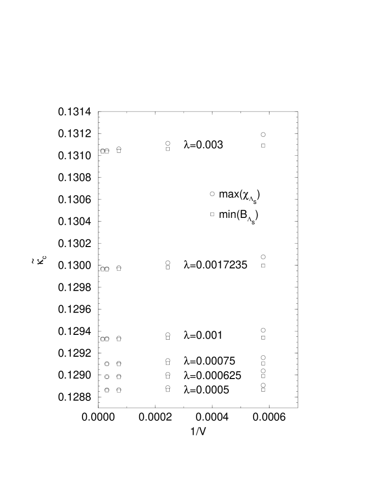
In Fig. 5 we summarize our results for the pseudo critical point obtained from the susceptibility and the Binder cumulant. In Table III we summarize estimates of the critical hopping parameter in the infinite volume obtained by a linear extrapolation of in using results of largest three volumes for each .
V Latent Heat
We calculate the latent heat with the equation [18],
| (7) |
where means the difference of in the pure symmetric phase and in the pure broken phase. It has been shown[1, 12] that the latent heat calculated with this equation is in good agreement with that obtained with the energy operator.
In order to calculate the expectation value in the pure phases, we separate the ensemble of configurations generated in a run into two sub-ensembles of pure phases. The division is made by inspecting the Monte Carlo time history of . In order to avoid contaminations from transition stages, iterations in those stages are removed following the method employed in Ref. [19].
A source of systematic error in the procedure above arises from the fact that the point of at which the run is performed does not exactly coincide with the pseudo critical point which we estimate from the susceptibility . In order to treat this problem we make two independent runs, both in the region of metastability, such that is sandwiched between the hopping parameter of the two runs. Then we interpolate results of the two runs for with a linear function of to . The error of the latent heat is calculated from those of and .
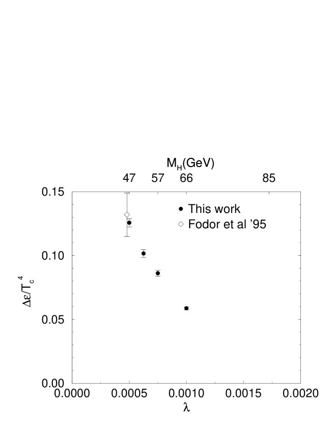
The result of our analysis is shown in Fig. 6. At the lightest Higgs boson mass of GeV our result is in good agreement with that of Ref. [11] obtained with the energy operator. The latent heat decrease apparently linearly with an increasing Higgs boson mass . A linear extrapolation of our data is consistent with a vanishing of the latent heat at GeV.
VI Interface Tension
The interface tension provides another indicator of the strength of the first-order transition. We calculate this quantity with the Binder’s histogram method [20]. Let and be the peak and valley height of the distribution of , reweighted such that the two peaks have an equal height. Define . For spatially cubic lattices used in our simulations, finite-size formula for the true interface tension is given by [21]
| (8) |
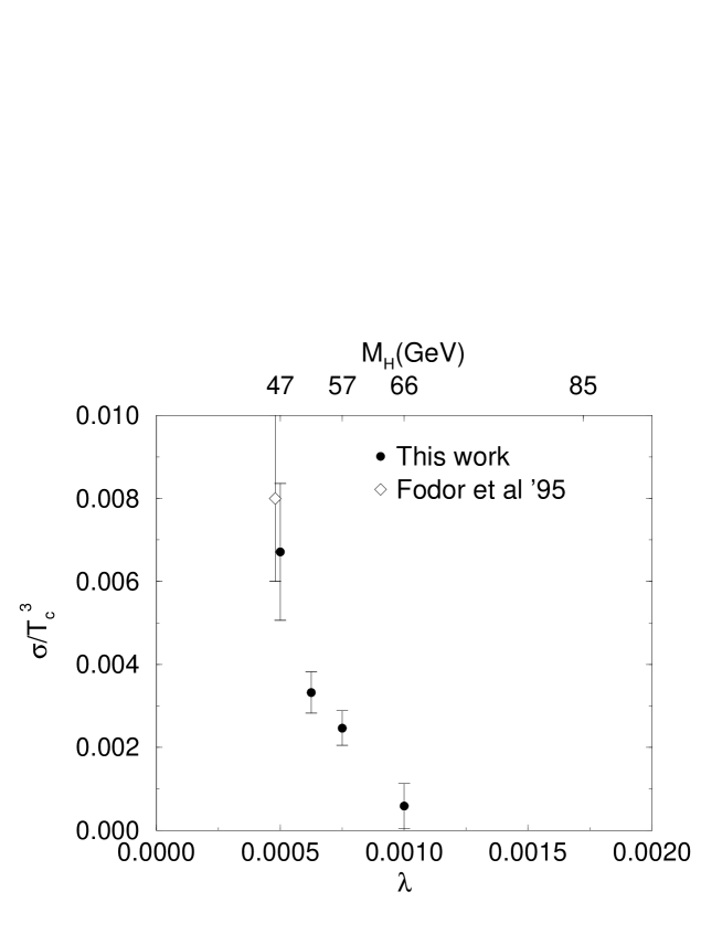
where is a constant independent of . Making a two parameter fit of obtained for the largest three volumes for GeV or two volumes for GeV we find shown in Fig. 7. The interface tension rapidly decrease with an increasing Higgs boson mass and seems to vanish around GeV as in the case of the latent heat.
VII Summary
Our finite-size scaling study establishes a first-order transition for GeV. For larger Higgs boson masses a rapid weakening of the transition makes it difficult to draw a definitive conclusion on the order within the range of lattice volumes employed in our simulation. However, combining finite-size data with results for the latent heat and the interface tension, our four-dimensional study suggests that the first-order transition terminates around GeV in the SU(2) gauge-Higgs model. This is consistent with the results of recent finite-size scaling studies carried out in the dimensionally reduced three-dimensional model[4, 7].
Acknowledgements
I would like to thank Akira Ukawa for useful discussions. The numerical calculations were carried out on VPP/500 at Science Information Processing Center of University of Tsukuba and at Center for Computational Physics at University of Tsukuba.
A
In Table I we listed the zero temperature Higgs boson mass and the critical temperature for each at our critical hopping parameter on the lattice. Here we describe how we estimated those values.
In Table IV we summarize published results for and at five different values of reported in Refs. [8, 11, 12]. Two values of employed in our simulation ( ) are among those in Table IV. For these cases we adopt the published results for and . For the other four values of we estimate and by an interpolation of results in Table IV.
At the tree revel the mass ratio is proportional to (the gauge coupling is fixed to in our simulations). Plotting five values of in Table IV against we find that they exhibit a smooth increase suitable for an interpolation. A cubic polynomial of yields a good fit with . We then estimate the values of at from the value of the fitted curve at where is the critical point determined from the susceptibility of listed in Table III. One can also make a fit with a quadratic polynomial (). The difference of values of from the two fits may be used as a measure of the systematic error of our estimation procedure. However, the difference is quite small ( ) compared with the statistical error (), and we adopt the statistical error in our estimate.
The results for the critical temperature has a sharp bend for large . Hence this variable is not suitable for interpolation of . We find, however, that as a function of is smoothly increasing, and a cubic polynomial fit goes well (). We use the fitted curve and the values of estimated above to find the values of . Fit with a quadratic polynomial () is used to estimate the systematic error, which turns out to be comparable to the statistical one. Those errors are combined into the final value of error shown in Table I.
REFERENCES
- [1] K. Jansen, Nucl. Phys. B (Proc. Suppl.) 47, 196 (1996).
- [2] K. Rummukainen, Proceedings of Lattice 96, to appear in Nucl. Phys. B (Proc. Suppl.) [hep-lat/9608079].
- [3] K. Kajantie, K. Rummukainen and M. Shaposhnikov, Nucl. Phys. B407, 356 (1993); K. Farakos, K. Kajantie, K. Rummukainen and M. Shaposhnikov, Phys. Lett. B 336, 494 (1994); K. Kajantie, M. Laine, K. Rummukainen and M. Shaposhnikov, Nucl. Phys. B466, 189 (1996).
- [4] K. Kajantie, M. Laine, K. Rummukainen and M. Shaposhnikov, Phys. Rev. Lett. 77, 2887 (1996).
- [5] E.-M. Ilgenfritz, J. Kripfganz, H. Perlt and A. Schiller, Phys. Lett. B 356, 561 (1995); M. Gürtler, E.-M. Ilgenfritz, J. Kripfganz, H. Perlt and A. Schiller, hep-lat/9512022; hep-lat/9605042.
- [6] F. Karsch, T. Neuhaus, A. Patkós and J. Rank, Nucl. Phys. B474, 217 (1996).
- [7] F. Karsch, T. Neuhaus, A. Patkós and J. Rank, Proceedings of Lattice 96, to appear in Nucl. Phys. B (Proc. Suppl.) [hep-lat/9608087].
- [8] B. Bunk, E.-M. Ilgenfritz, J. Kripfganz and A. Schiller, Phys. Lett. B 284, 371 (1992).
- [9] B. Bunk, E.-M. Ilgenfritz, J. Kripfganz and A. Schiller, Nucl. Phys. B403, 453 (1993).
- [10] Z. Fodor, J. Hein, K. Jansen, A. Jaster, I. Montvay and F. Csikor, Phys. Lett. B 334, 405 (1994).
- [11] Z. Fodor, J. Hein, K. Jansen, A. Jaster and I. Montvay, Nucl. Phys. B439, 147 (1995).
- [12] F. Csikor, Z. Fodor, J. Hein, A. Jaster and I. Montvay, Nucl. Phys. B474, 421 (1996).
- [13] P. Janot, Nucl. Phys. B (Proc. Suppl.) 38, 264 (1995).
- [14] B. Bunk, Nucl. Phys. B (Proc. Suppl.) 42, 566 (1995).
- [15] Z. Fodor and K. Jansen, Phys. Lett. B 331, 119 (1994).
- [16] I.R. McDonald and K. Singer, Discuss. Faraday Soc. 43, 40 (1967); A.M. Ferrenberg and R. Swendsen, Phys. Rev. Lett. 61, 2058 (1988); 63, 1195 (1989).
- [17] For a review, see, M. N. Barber, in Phase Transitions and Critical Phenomena, Vol. 8, eds. C. Domb and J. Lebowitz (Academic Press, New York, 1983).
- [18] W. Buchmüller, Z. Fodor and A. Hebecker, Nucl. Phys. B447, 317 (1995).
- [19] Y. Iwasaki, K. Kanaya, T. Yoshié, T. Hoshino, T. Shirakawa, Y. Oyanagi, S. Ichii and T. Kawai, Phys. Rev. D 46, 4657 (1992).
- [20] K. Binder, Z. Phys. B 43, 119 (1981); Phys. Rev. A 25, 1699 (1982).
- [21] Y. Iwasaki, K. Kanaya, L. Kärkkäinen, K. Rummukainen and T. Yoshié, Phys. Rev. D 49, 3540 (1994).
| (GeV) | (GeV) | use | |||
|---|---|---|---|---|---|
| 0.0005 | 47(2) | 94(1) | 8 | 0.128950 | |
| 12 | 0.128900 | ||||
| 16 | 0.128883 | ||||
| 24 | 0.128866 | ||||
| 32 | 0.128860 | ||||
| 32 | 0.128862 | ||||
| 32 | 0.128865 | ||||
| 0.000625 | 52(1) | 100(3) | 8 | 0.129110 | |
| 12 | 0.129036 | ||||
| 16 | 0.129004 | ||||
| 24 | 0.128986 | ||||
| 32 | 0.128983 | ||||
| 32 | 0.128987 | ||||
| 0.00075 | 57(1) | 107(3) | 8 | 0.129243 | |
| 12 | 0.129158 | ||||
| 16 | 0.129126 | ||||
| 24 | 0.129103 | ||||
| 32 | 0.129098 | ||||
| 32 | 0.129102 | ||||
| 32 | 0.129106 |
| (GeV) | (GeV) | use | |||
|---|---|---|---|---|---|
| 0.001 | 66(2) | 119(3) | 8 | 0.129476 | |
| 12 | 0.129407 | ||||
| 16 | 0.129349 | ||||
| 24 | 0.129330 | ||||
| 32 | 0.129328 | ||||
| 40 | 0.129327 | ||||
| 40 | 0.129330 | ||||
| 0.0017235 | 85(3) | 139(2) | 8 | 0.130200 | |
| 12 | 0.130080 | ||||
| 16 | 0.130026 | ||||
| 24 | 0.129980 | ||||
| 32 | 0.129966 | ||||
| 40 | 0.129968 | ||||
| 0.003 | 108(6) | 157(10) | 8 | 0.131350 | |
| 12 | 0.131050 | ||||
| 12 | 0.131200 | ||||
| 16 | 0.131111 | ||||
| 24 | 0.131065 | ||||
| 32 | 0.131054 | ||||
| 40 | 0.131042 |
| heat bath | overrelaxation | |||
|---|---|---|---|---|
| 1 | 4 | 3 | 3 | 1 |
| 0.0005 | 0.000625 | 0.00075 | 0.001 | 0.0017235 | 0.003 | |
|---|---|---|---|---|---|---|
| () | 0.1288607(23) | 0.1289812(11) | 0.1290981(14) | 0.1293262(11) | 0.1299633(29) | 0.1310360(40) |
| () | 0.1288584(13) | 0.1289822(25) | 0.1290974(14) | 0.1293266(11) | 0.1299622(27) | 0.1310318(34) |
| (GeV) | (GeV) | reference | ||
|---|---|---|---|---|
| 0.0001 | 0.1283 | 18(1) | 38(1) | [11] |
| 0.0003 | 0.12865 | 35(1) | 71(1) | [12] |
| 0.0005 | 0.12885 | 47(2) | 94(1) | [11] |
| 0.0017235 | 0.13 | 85(3) | 139(2) | [8] |
| 0.023705 | 0.145 | 196(13) | 185(4) | [8] |