HUB–EP–96/59
revised
Topology at the Deconfinement Transition
Uncovered by Inverse Blocking
in $SU(2)$ Pure Gauge Theory
with Fixed Point Action

Abstract

Renormalization group transformations as discussed recently in deriving fixed point actions are used to analyse the vacuum structure near to the deconfinement temperature. Monte Carlo configurations are generated using the fixed point action. We compare equilibrium configurations with configurations obtained by inverse blocking from a coarser lattice. The absence of short range vacuum fluctuations in the latter does not influence the string tension. For the inversely blocked configurations we find the following: (i) the topological susceptibility $\chi_{top}$ is consistent with the phenomenological value in the confinement phase, (ii) $\chi_{top}$ drops across the deconfinement transition, (iii) density and size of instantons are estimated, (iv) the topological density is found to be correlated to Abelian monopole currents and (v) the density of spacelike monopole currents becomes a confinement order parameter.

1 Introduction

Not much is known from first principles about the topological structure at the thermal phase transition in Quantum Chromodynamics. How this structure changes at the deconfinement phase transition is not even clear in pure gauge theory. What we mean by ”topological structure” is the characterization of Euclidean field trajectories in terms of instantons [1, 2] and Abelian monopoles [3, 4] and their interrelation. Changes of this structure are expected to be the common mechanism for deconfinement and restoration of chiral symmetry. Understanding this mechanism is important for understanding the QCD vacuum.

There was a wave of attention recently for improving lattice actions for gauge fields [5] (and fermions). Part of the interest was motivated to minimize finite lattice spacing corrections in simulation results obtained on coarse lattices. One particular approach towards improvement was guided by the desire to construct a perfect action being a fixed point action [6, 7] with respect to some real space renormalization group (RG) transformations. In this context the concept of inverse blocking came up which is the essence of a new method, recently proposed by DeGrand et al. [8, 9]. In particular it improves the determination of the topological charge of a lattice configuration.

In the present paper we want to explore the capability of this method, to resolve more details and different aspects of topological structure. In the neighbourhood of the deconfinement transition of the pure $SU(2)$ gauge theory, we want to study the space-time distribution of topological charge, correlations of the density with itself and with Abelian monopole currents.

The topological charge density, when defined for quantum fields, is obscured by ultraviolet fluctuations which must be removed in some way. Cooling [10] has been invented for this purpose long ago. According to the Abelian dominance scenario at large distances [3, 4] Abelian magnetic monopoles are closely related to confinement. The density [11] and anisotropy [12] of these magnetic currents are studied in the maximally Abelian gauge [13]. These currents are quantized by construction [14]. This does not exclude the possibility that some part of these currents are lattice artefacts which do not correspond to long distance physics. Correlations indicating a close relation between topological charge and Abelian magnetic monopole currents have been studied, not addressing this question. They have been studied so far for particular instanton configurations [15] and, as far as the quantized vacuum is concerned, the cooling method has been employed [16]. However, cooling is known to change the topological structure and has to be used with care.

A closer examination shows that the method of Refs. [8, 9] gives not only the topological charge but also permits a reasonable definition of the topological density of generic, equilibrium lattice fields with minimal effort. A better resolution of topological and monopole structure is possible without recourse to cooling. While the method is applied to extract the topological structure, the monopole activity is changed, too, roughly in proportion to the topological activity (to be defined below). We shall see that part of it becomes an order parameter of the confinement/deconfinement transition, according to the alleged role monopoles play for confinement.

According to the scope of our present study, let us sketch the background of this approach [6] restricting the discussion to the case of pure gauge field theories. The starting point is a block spin transformation (here of scale factor two) which maps a fine lattice configuration of link matrices $U_{x,\mu}$ to a coarse lattice configuration with link matrices $V_{x,\mu}$ (each single link being an element of the gauge group $SU(N)$). The second ingredient is a general type of action $S_{FP}$, written on both lattices in terms of Wilson loops (evaluated in various representations). The classical perfectness of this action is guaranteed if there exists an inverse blocking transformation $~{}V\rightarrow U~{}$ with respect to which the action saturates the inequality

$$~{}~{}~{}~{}~{}~{}~{}~{}S_{FP}(U)+\kappa~{}T(U,V)\geq S_{FP}(V)~{}~{}.$$ (1)

Here, $T(U,V)$ is some non-negative functional related to the blockspin transformation and $\kappa$ is a kind of Lagrange multiplier. Once the action and other parameters have been determined, this inequality leads to the target configuration $~{}U$ of the inverse blocking by minimization of the l. h. s., the fixed point action with respect to $~{}U$, with a constraint derived from the coarse configuration $~{}V$. Thus, $~{}U$ is found as the result of an iterative relaxation process and cannot be explicitely expressed. We call the mapping $~{}V\rightarrow U$ one step of inverse blocking. Similar to blocking, inverse blocking can be iterated. This leads to a sequence of interpolating configurations on finer and finer lattices.

Without giving details, we mention that the saturated inequality (1) is constructive for finding the perfect action itself. It has been used [8] to optimize the ratios between the couplings in front of various loops in different representations within the fixed point action $S_{FP}$, as well as the other constants related to the block spin transformation.

After this machinery has been set up, the procedure of inverse blocking remains a useful tool of analysis. Doing a sequence of inverse blocking steps one would be able to relate a continuum configuration to any given lattice configuration. The topological charge of this continuum configuration is the topological charge related to the given lattice configuration (the classically perfect topological charge). This prescription is an important conceptual step forward compared with previous techniques of measuring topological charge on the lattice, eventually used in combination with cooling.

Inverse blocking has been used before [8, 9] only to measure the topological charge of lattice configurations, by evaluating the Phillips–Stone (PS) charge [17] just on the next finer level. The success indicates that one step of inverse blocking can be sufficient to have access to the classically perfect topological charge corresponding to the continuum by means of a lattice definition. Other lattice algorithms besides PS could also have been used, for instance in order to test the uniqueness of charge. We will use in this paper a geometric charge due to Lüscher [18, 19] and the old plaquette based (field theoretic or naive) definition [20, 21]. Both have the advantage to localize the topological density in space-time which makes them suitable for our present purpose.

The first concern in Ref. [8] has been that action and topological charge of artificially constructed lattice instantons should be independent of size, if the perfect action is used and the topological charge is measured as described. This was demonstrated for instanton configurations with $\rho>0.8\cdot a$. There were no dislocations, with action $S/S_{I}<6/11$ (entropic bound, instanton action $S_{I}=2\pi^{2}$) and non–zero topological charge, among them. However, the perfect action and the new definition of topological charge are useful also at finite $\beta$. In the second paper [9] a (truncated) fixed point action has been successfully tested for scaling of the deconfinement temperature, of the torelon mass, of the string tension and of the topological susceptibility. For the latter, it has been stressed that inverse blocking has been indispensable to achieve reasonable scaling. This has nourished the hope that the fixed point action and the inverse blocking prescription for the topological charge can avoid dislocations which otherwise (for instance in the case of Wilson’s action) are known to spoil the continuum limit of the topological susceptibility [22].

Even the temperature dependence of the topological susceptibility has remained controversial until recently. Armed with the new method, the topological susceptibility has been measured across the deconfinement transition [9] without the ambiguities of the cooling method [23, 24]. Inverse blocking is not the only technique to avoid cooling. We only want to mention the use of an improved lattice operator of the topological density [25]. This approach has given a much more discontinuous drop [26] at the deconfinement transition than the inverse blocking method [9].

Our paper is organized as follows. In section 2 we give details on the fixed point action, on blocking and inverse blocking. In section 3 we present results on the string tension. For symmetric lattices this serves to calibrate the lattice step size $a(\beta)$ in accordance to simulations using the fixed point action. The finite temperature string tension is computed (in the confined phase) from Polyakov line correlators. These results are indicating that the string tension is largely conserved by inverse blocking. Section 4 contains our results on the gross topological features. The topological susceptibility obtained on inversely blocked configurations in the confined phase is quantitatively reasonable. The temperature dependence of the topological susceptibility across the phase transition is studied. Analysing inversely blocked configurations we observe, apart from the decay of the topological susceptibility, the complete suppression of spatial Abelian monopole currents in the deconfined phase. In section 5 we present results on topological charge density–density correlations and on monopole–instanton correlations. We visualize clusters of topological charge together with their accompanying monopole currents for typical confining configurations. In closing, directions for further work are pointed out in section 6.

2 Fixed Point Action and Inverse Blocking

2.1 Action and Blocking

The simplified fixed point action [9] is parametrized in terms of only two types of Wilson loops, plaquettes $U_{C_{1}}=U_{x,\mu,\nu}$ (type $C_{1}$) and tilted $3$-dimensional $6$-link loops (type $C_{2}$) of the form

$$U_{C_{2}}=U_{x,\mu,\nu,\lambda}=U_{x,\mu}U_{x+\hat{\mu},\nu}U_{x+\hat{\mu}+\hat{\nu},\lambda}U_{x+\hat{\nu}+\hat{\lambda},\mu}^{+}U_{x+\hat{\lambda},\nu}^{+}U_{x,\lambda}^{+}~{}~{}.$$ (2)

It contains several powers of the corresponding linear action terms as follows

$$S_{FP}(U)=\sum_{type~{}i}\sum_{C_{i}}\sum_{j=1}^{4}w(i,j)(1-{1\over 2}~{}{\mathrm{t}r}~{}U_{C_{i}})^{j}~{}~{}.$$ (3)

The parameter of this action have been optimized in Ref. [9] and are reproduced in Table 1.

$w(i,j)$	$j=1$	$j=2$	$j=3$	$j=4$
$i=1$ (plaquettes)	$.3333$	$.00402$	$.00674$	$.0152$
$i=2$ (6-link loops)	$.08333$	$.0156$	$.0149$	$-.0035$

Table 1: Weight coefficients of the simplified fixed point action

The notion of blocking is recalled here in order to define some notations. Fat links $V_{x,\mu}$ are defined for $x_{\nu}=odd$ for all $\nu=1,2,3,4$ only. These are the nodes of the blocked lattice. The blocking transformation expresses a fat link in terms of the product of the two links along the fat link plus a sum over six rectangular $4$-link staples passing by the fat link:

$$\tilde{V}_{x,\mu} = c_{1}^{block}~{}U_{x,\mu}U_{x+\hat{\mu},\mu}$$

$$+\sum_{\nu\neq\mu}c_{2}^{block}\left(U_{x,\nu}U_{x+\hat{\nu},\mu}U_{x+\hat{\nu}+\hat{\mu},\mu}U_{x+2\hat{\mu},\nu}^{+}\right.$$

$$~{}~{}~{}~{}~{}~{}~{}~{}+\left.U_{x-\hat{\nu},\nu}^{+}U_{x-\hat{\nu},\mu}U_{x-\hat{\nu}+\hat{\mu},\mu}U_{x-\hat{\nu}+2\hat{\mu},\nu}\right).$$

The actual fat link $V_{x,\mu}$ is then obtained by normalization to $SU(2)$:

$$V_{x,\mu}={{\tilde{V}_{x,\mu}}\over{\sqrt{{\mathrm{d}et}\left(\tilde{V}_{x,\mu}\right)}}}.$$ (5)

The following blocking parameters have been recommended for this type of RG transformation in Ref. [27]

$$c_{2}^{block} = 0.12$$

$$c_{1}^{block} = 1-6~{}c_{2}^{block}~{}~{}.$$ (6)

2.2 Inverse Blocking

Inverse blocking consists in searching the constrained minimum with respect to the fine links $~{}U$ of an extended action

$$~{}~{}~{}S_{ext}(U)=S_{FP}(U)+\kappa~{}T(U,V)~{}~{},$$ (7)

which includes, besides of the fixed point action $S_{FP}$, the blocking kernel

$$T(U,V)=\sum_{fat~{}links}\left(\max_{W\epsilon SU(2)}\left({\mathrm{t}r}\left(W^{+}\tilde{V}\right)\right)-{\mathrm{t}r}\left(V^{+}\tilde{V}\right)\right)\geq 0$$ (8)

with $\kappa$ as a Lagrange multiplier. For better readability, we have dropped the labels $x,\mu$ of the fat links $V_{x,\mu}$ (describing the blocked configuration) and of the $\tilde{V}_{x,\mu}$. The latter are expressed in terms of the fine $~{}U$’s exactly as in (2.1) and are not related to $V_{x,\mu}$ in the present context.

For comparison, cooling the gauge field configuration $~{}U$ means to minimize the new action with $\kappa=0$. The result of cooling is no more influenced by the coarse configuration $~{}V$ in the process of relaxation. The unconstrained minimum $~{}U$ is a classical solution on the lattice with respect to $S_{FP}$. It can only depend on the initial configuration if that determines a non–trivial basin of attraction.

Concerning the organization of measurements, we differ from DeGrand et al. They have simulated on the coarse lattice, using the fine lattice only for measuring the topological charge on the inversely blocked configurations. The coarse lattice was their reference scale. We carried out simulations on the fine lattice (at some lattice scale $~{}a$) chosing a $\beta$–value to produce a Monte Carlo ensemble of gauge field configurations $U^{MC}$ according to the fixed point action. Most of these configurations have been used only for comparison as described below. Another part of them (in a separate run with the same $\beta$) has been used to produce an ensemble of coarse lattice configurations $~{}V$ by blocking the fine lattice configurations. Due to variance reduction it was possible to restrict this second ensemble to considerably less configurations than the other. At scale $~{}2\cdot a~{}$ (and bigger) the coarse ensemble is expected to describe the same physics as the fine ensemble. We could have asked to which $\beta^{\prime}$ the coarse lattice configurations correspond. However, for the sake of clarity in the comparison we always refer to the original $\beta$–value and $a$ as our reference scale. The coarse lattice configurations $~{}V$ have been analyzed with respect to their topological properties by inverse blocking, $~{}V\rightarrow U^{IB}$.

To create the coarse configurations by blocking from another equilibrium ensemble is no matter of principle. It is, however, an advantage to keep the Monte Carlo configuration on the fine lattice in order to use it as a start configuration for the constrained minimization. Due to this particular circumstance the inversely blocked configuration $U^{IB}$ can be imagined as a smoothed copy of the original configurations $U^{MC}$. Nevertheless, it can exhibit no other topological structure than present in the blocked configuration $~{}V$ (which influences the relaxation through the blocking functional $\kappa T(U,V)$). In what follows we shall denote the combined application of one step of blocking followed by one step of inverse blocking as smoothing.

Classical configurations are particular. Instanton solutions on the fine lattice are always reproduced under smoothing. Their topological structure is the same on the coarse and the fine lattices. Not only the action is recovered but also the shape of the topological charge distribution and the location of monopole currents. We have produced a set of almost classical configurations by cooling from hot starts using the simplified fixed point action (3). This set has then been used for testing our code of the smoothing algorithm. If one blocks a classical solution, one finds $S_{FP}(U)=S_{FP}(V)$.

However, this technique is intended to be applied to non–classical configurations. Before entering our investigations, we have tested, creating fine lattice configurations $U^{MC}$ (Monte Carlo generated with $S_{FP}$ at various $\beta$–values) and blocking them into coarse configurations $~{}V$, which $\kappa$–value must be used in the extended action (7) driving $~{}U$ from $U^{MC}$ to $U^{IB}$. The relaxed configurations $U^{IB}$ should turn the inequality (1) into an equality relating $U^{IB}$ to $~{}V$. Under these circumstances we were not able to confirm the Lagrange multiplier $\kappa=12$ recommended in Ref. [27] (for the given type of RG transformation in $SU(3)$). Instead, we have found that a choice $\kappa=5.15$ (slightly depending on $\beta$) is suitable, throughout the $\beta$ range under study, to guarantee the equality in (1) within an accuracy of one to three per cent. We have adopted the fixed point action but decided to use our empirical value for $\kappa$. In principle, $\kappa$ and the parameters of the fixed point action are closely tied together. They should be optimized w. r. t. (1) using an ensemble of configurations created with exactly this action. This is a much more ambitious project than it has been pursued until now. The authors of Ref. [8] are continuing this program. This whole discussion puts a question mark on the exact relation between the action and $\kappa$. Also in view of this, we consider the results of the present paper as exploratory.

Knowing the extended action (7) we can distinguish three types of links on the fine lattice. Links along the fat links and links lying inside coarse plaquettes contribute to $\tilde{V}$ and are updated (relaxed) with respect to $S_{ext}$. All other fine links are not subject to constraints and are updated with respect to $S_{FP}$ alone.

Figure 1: Relaxation towards the inversely blocked configuration vs. cooling for a typical Monte Carlo configuration generated at $\beta=1.5$ on a $12^{3}\times 4$ lattice

A typical relaxation process is shown in Fig. 1. The upper curve demonstrates how the extended action $S_{FP}(U)+\kappa~{}T(U,V)$ decays versus number of iterations. The upper horizontal line marks the action of the original Monte Carlo generated configuration $S_{FP}(U^{MC})$, the lower horizontal the action of the blocked configuration $S_{FP}(V)$. After $~{}V$ has been obtained from $U^{MC}$ by blocking and one has plugged in $U^{MC}$ into the extended action $S_{ext}(U)$, $T(U,V)$ vanishes by construction. Therefore the minimization of $S_{ext}$ starts at the level of $S_{FP}(U^{MC})$. After the constrained minimum configuration $U^{IB}$ has been found, the extended action is shared between the fixed point action $S_{FP}(U^{IB})$ and the functional $\kappa~{}T(U^{IB},V)$. In Fig. 1 the history of $S_{FP}(U)$ is separately recorded by the curve in the middle. The lowest curve shows how $S_{FP}(U)$ would evolve under cooling (with $\kappa$ put to zero). After $20$ iterations the unconstrained relaxation runs into configurations $~{}U$ with a fixed point action $S_{FP}(U)$ one order of magnitude below $S_{FP}(U^{IB})$ and the action decays further. On the other hand, this demonstrates that inverse blocking does not need huge numbers of iterations to achieve convergence if a good start configuration is known. A particular relaxation scheduling, for instance a modification of the action during the first iterations, is not necessary.

3 String Tension at $T=0$ and Finite
Temperature

The inverse coupling constant $\beta$ enters through the Gibbs weight

$$Z=\int DU\exp(-\beta S_{FP}(U))$$ (9)

into the creation of fine lattice configurations. It defines the scale through the lattice spacing $a(\beta)$. We wanted to compare the naive charge with Lüscher’s charge which is, similar to the fixed point action, very CPU intensive. Therefore we have restricted ourselves to a fine lattice of size $12^{3}\times 4$ for the finite temperature part of these explorative investigations.

For $L_{t}=4$ the deconfinement transition was known to occur at $\beta_{c}=1.575(10)$ [9]. This has been established by the crossing of the Binder cumulants of the Polyakov line for several spatial lattice sizes. We have not attempted here to improve the localization of the deconfining transition or to do a finite size analysis. Rather than doing that, we have simulated at $\beta$–values safely lower ($\beta=1.40$, $\beta=1.50$ and $\beta=1.54$) and higher ($\beta=1.61$ and $\beta=1.80$) than the deconfinement transition.

3.1 Lattice Spacing from the Zero Temperature
String Tension

In order to measure the lattice spacing $a$ at each of the $\beta$–values to be used in the finite temperature simulations we have complementarily measured the zero temperature string tension on a $12^{4}$ lattice. No topological features have been analysed in this part of our calculations.

$\beta$	$1.40$	$1.50$	$1.54$	$1.60$	$1.80$
Monte Carlo	$0.445(8)$	$0.245(3)$	$0.193(3)$	$0.124(2)$	$0.0380(9)$
inv. blocked	$0.228(4)$	$0.182(1)$	$0.156(3)$	$0.108(3)$	$0.0299(1)$
Monte Carlo	$152(3)$	$135(2)$	$129(2)$	$111(2)$	$91.7(19)$
inv. blocked	$77.9(10)$	$100.5(10)$	$104.5(20)$	$96.8(20)$	$71.2(20)$

Table 2: String tension $\sigma~{}a^{2}$ (above) and $\sigma/\Lambda_{L}^{2}$ (below) at zero temperature from fuzzy Wilson loops in axial gauge on a $12^{4}$ lattice (with two–loop expression for $a(\beta)\Lambda_{L}$)

The string tension has been obtained for Monte Carlo configurations in the axial gauge from smeared Wilson loops. The same has been measured on smoothed configurations for comparison. The axial gauge is enforced in chronological order time slice by time slice (except for the last one) after a certain direction has been chosen as Euclidean time. This is done putting each temporal link $U_{4}(x)$ equal to unity by applying a suitable gauge transformation $g(x+\hat{4})$ at the end of that link. Smearing [28] has been applied to configurations in this gauge. This is an iterative operation (without change of scale) replacing each spatial link $~{}U$ by $U^{smear}$ through a procedure similar to (2.1) (since without change of scale, with only one step in $\mu=1,2,3$ direction and with only spatial staples involved, $\nu=1,2,3~{}~{}\nu\neq\mu$). In the axial gauge, timelike parts of the Wilson loops are mostly equal to unity (if they do not contain links from the last to the first time slice). Smearing effectively replaces the fixed–time parts of planar Wilson loops by weighted sums over paths, running from the quark to the antiquark site (a distance $R$ apart). The temporal extension of the Wilson loop is denoted as $T$. In view of the maximal spatial distance $R=6$ of quark and antiquark, we have applied $N_{smear}=6$ smearing iterations with an optimal smearing parameter (the notation is as in (2.1) )

$$c_{2}^{smear} = 0.125$$

$$c_{1}^{smear} = 1-4~{}c_{2}^{smear}.$$ (10)

This parameter had been optimized in order to get an early plateau in $T$ of $\log(W(R,T+1)/W(R,T)$ for the Monte Carlo configurations at $\beta=1.5$. For simplicity, it has been applied in all measurements of the zero temperature string tension.

The potential is fitted (for all $R$) from exponential fits over the range $T=2...5$. For the inversely blocked configurations we have restricted the fit range to $T=3...5$. The potential $V(R)$ has been fitted with a $3$-parameter fit that includes a constant, Coulomb and linear part over the range $R=1...5$. For the inversely blocked configurations the Coulomb part is consistent with zero. The string tension is obtained from the linear part of the potential. The $\beta$ dependence and the comparison between normal Monte Carlo configurations and inversely blocked (smoothed) configurations is presented in Table 2.

The string tension for inversely blocked configurations has a scaling window (assuming asymptotic scaling with the two–loop $a(\beta)$) including our measurements from $\beta=1.5$ to $\beta=1.6$. The string tension measured at $\beta=1.8$ suffers from a small volume effect, since the spatial box size at this $\beta$ is physically not larger than $2.35/T_{c}$. For definiteness, we choose the string tension from the Monte Carlo configurations in order to express non–perturbatively $a(\beta)$ and the $4$-volume of the lattice through the invariant string tension.

According to the RG philosophy the same large scale physics should be represented by the coarse configurations (if obtained by blocking) and the original Monte Carlo configurations (on the fine lattice), as long as the blocking scale is still safely separated from the physical scale under investigation. It is not clear a priori that the inversely blocked configurations $U^{IB}$ still contain the same large scale physics. In case of the string tension this could only be the case if it decouples from the ultraviolet fluctuations. In order to test this it makes sense to compare the string tensions of Monte Carlo and inversely blocked configurations at various $\beta$. The string tension is built up at large distances and is expected to coincide for both types of configurations, while the perturbative Coulomb part of the potential is not expected to survive inverse blocking. We compare in table 2 the zero temperature string tension as found on Monte Carlo and inversely blocked configurations, both on the fine lattice. We find our expectation largely confirmed. The string tension of inversely blocked configurations is somewhat smaller ($75$ to $90$ per cent depending on $\beta$) than the string tension of normal Monte Carlo configurations.

The exception at the lowest $\beta=1.4$ can be explained by the fact that at very strong coupling the blocking scale interferes with the confinement scale. This is supported by the observation that also the topological structure is not truly captured. This becomes obvious if one shifts the coarse lattice (in one of the $2^{4}-1$ directions) relative to the fine lattice. This is the reason why we must exclude the lowest $\beta$-value also from extracting the temperature dependence of the topological susceptibility.

This is place to compare cooling and inverse blocking as far as the string tension is concerned. Cooling conserves the string tension [29] as a function of the cooling steps only as long as the topological susceptibility goes through a plateau. The topological susceptibility is defined as the plateau value in this method [30]. Cooling as used by the MIT group [31] in order to measure hadronic correlation functions goes much farther and does not conserve the string tension.

3.2 Is the $T\neq 0$ String Tension Changing under
Inverse Blocking ?

We discuss now our results concerning the temperature dependent string tension $\sigma(T)$. Although this is not our main interest, we want to see to what extent this quantity is also insensitive to inverse blocking. The configurations are Monte Carlo generated on asymmetric lattices of size $12^{3}\times 4$. The string tension $\sigma(T)$ should vanish in the deconfinement phase, at $\beta>\beta_{c}$. A suitable definition of the string tension for thermal lattices is provided by the correlator of Polyakov lines

$$L({\bf x})={\mathrm{t}r}\prod_{t=1}^{L_{t}}U_{\bf{x}t,4}$$ (11)

which, in the confinement phase, exhibits the confining potential in the form

$$\langle L({\bf 0})L({\bf x})\rangle\propto\exp(-V_{\overline{q}q}^{conf}({\bf x})/T)$$ (12)

where $V_{\overline{q}q}^{conf}({\bf x})\sim\sigma(T)|{\bf x}|$ at large distances. $V_{\overline{q}q}^{conf}({\bf x})$ contains the self–energies of $q$ and $\overline{q}$ and the perturbative Coulomb potential, too. These are expected to change under inverse blocking.

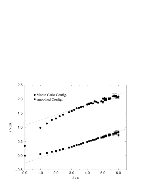
Figure 2: $\overline{q}q$ potential from Polyakov line correlators for Monte Carlo (above) and inversely blocked configurations at $\beta=1.5$ in the confinement phase

In the measurement of Polyakov lines and their correlators there is no place for smearing and no sense in performing the axial gauge. The normalized correlators in the Monte Carlo and the inversely blocked ensemble can be

$\beta$	$1.40$	$1.50$	$1.54$
$T/T_{c}$	$0.656$	$0.834$	$0.919$
Monte Carlo	$0.253(23)$	$0.193(4)$	$0.176(5)$
inv. blocked	$0.242(8)$	$0.189(2)$	$0.137(3)$
Monte Carlo	$86(8)$	$110(4)$	$118(4)$
inv. blocked	$83(3)$	$104(2)$	$92(2)$

Table 3: String tension $\sigma(T)~{}a^{2}$ (above) and $\sigma(T)/\Lambda_{L}^{2}$ (below) from Polyakov line correlators at various temperatures $T<T_{c}$ in the confinement phase (with two–loop expression for $a(\beta)\Lambda_{L}$)

directly compared for the three $\beta$–values that belong to the confinement phase. Fig. 2 shows for $\beta=1.5$ the logarithm of the (suitably normalized) Polyakov line correlator as function of the distance. In Table 3 we collect the extracted values of the string tension at the three temperatures in the confinement phase for Monte Carlo and inversely blocked configurations. There is an interesting temperature dependence of the thermal string tension, but no big difference between the string tensions measured on the Monte Carlo and the inversely blocked ensemble. The reduction is less than $5$ per cent at temperatures $T<0.8~{}T_{c}$ and grows to more than $20$ per cent at $T>0.9~{}T_{c}$. We observe also at $T<T_{c}$ that the original Monte Carlo string tension is practically the same as the string tension measured on the much smoother inversely blocked configurations and seems to be independent of the short range fluctuations.

4 Gross Topological Features Near to the
Deconfinement Transition

The first measurement of topological features of pure $SU(2)$ gauge theory with the new method concerns the temperature dependence of the topological susceptibility of pure $SU(2)$ gauge theory, here over the range from $0.8~{}T_{c}$ to $1.7~{}T_{c}$. This question has been studied already in Ref. [9] on lattices of invariable spatial size (both in lattice units $L_{s}$ and physical units) by varying the temporal extent $L_{t}$. We keep the lattice size invariantly equal to $12^{3}\times 4$ while varying $\beta$. This additional measurement might be of interest as such since now the spatial size changes with the temperature.

4.1 Topological Susceptibility Across the Deconfining
Phase Transition

We have measured on Monte Carlo configurations (separated by $20$ updates) on the lattice $12^{3}\times 4$ the topological charges according to Lüscher’s definition, $Q_{Luescher}$[18, 19], and using the naive topological density [20]. The latter is defined (actually in a symmetrized way) in terms of plaquettes

$$q_{naive}(x)=-\frac{1}{2^{9}\pi^{2}}\sum_{\mu,\nu,\sigma,\rho=-4}^{+4}\epsilon_{\mu\nu\sigma\rho}{\mathrm{t}r}\left(U_{x,\mu,\nu}U_{x,\sigma,\rho}\right)$$ (13)

with

$$Q_{naive}=\sum_{x}q_{naive}(x)$$ (14)

(summed over lattice points). The statistics of analyzed Monte Carlo configurations amounts to $300$ configurations. These measurements will be confronted for each $\beta$ with corresponding ones on an independent ensemble of $100$ inversely blocked (smoothed) configurations. There is no room for details of Lüscher’s charge [19]. Important for us is that it is also written as a sum of localized contributions

$$Q_{luescher}=\sum_{x}q_{luescher}(x)$$ (15)

(summed over hypercubes). The time consuming part of this algorithm is the numerical integration of $2$- and $3$-dimensional integrals. It should be encouraging that evaluating the topological charge of inversely blocked configuration needs only $\frac{1}{10}$ of CPU time (function calls) compared to Monte Carlo configurations. The topological susceptibility is defined as

$$\chi_{top}={{\langle Q^{2}\rangle}\over{N_{sites}a^{4}}},$$ (16)

with total charges $Q$ corresponding here always to the naive and Lüscher’s charge. $N_{sites}$ is the number of lattice points $L_{s}^{3}\times L_{t}$ and we estimate the physical lattice volume $N_{sites}a^{4}$ with the help of the zero temperature string tension. Data for Monte Carlo and inversely blocked configurations as function of $T/T_{c}$ (yet without renormalization of the naive topological susceptibility) are collected in Table 4.

$\chi_{top}$	$\beta$	$T/T_{c}$	$\chi_{top}^{luescher}/\Lambda_{L}^{4}$	$\chi_{top}^{naive}/\Lambda_{L}^{4}$
Monte Carlo	$1.40$	$0.656$	$0.224(17)10^{4}$	$0.146(12)10^{2}$
	$1.50$	$0.834$	$0.287(24)10^{4}$	$0.370(27)10^{2}$
	$1.54$	$0.919$	$0.310(27)10^{4}$	$0.449(43)10^{2}$
	$1.61$	$1.089$	$0.235(19)10^{4}$	$0.753(59)10^{2}$
	$1.80$	$1.732$	$0.190(16)10^{4}$	$0.308(24)10^{3}$
inv. blocked	$1.40$	$0.656$	$0.127(17)10^{3}$	$0.84(11)10^{2}$
	$1.50$	$0.834$	$0.358(47)10^{3}$	$0.240(29)10^{3}$
	$1.54$	$0.919$	$0.324(43)10^{3}$	$0.239(30)10^{3}$
	$1.61$	$1.089$	$0.138(25)10^{3}$	$0.962(18)10^{2}$
	$1.80$	$1.732$	$0.164(11)10^{2}$	$0.100(70)10^{2}$

Table 4: Topological susceptibilities in the Monte Carlo and inversely blocked samples (with two–loop expression for $a(\beta)\Lambda_{L}$)

Only the topological susceptibility $\chi_{top}^{luescher}$ of the inversely blocked ensemble can be interpreted as a topological susceptibility (in the sense of the classically perfect topological charge). We have to agree that the topological charges belong to the coarse lattice and are defined at a scale given by the coarse lattice spacing. The apparent topological susceptibility evaluated on the Monte Carlo ensemble of fine lattice configurations is bigger than $\chi_{top}^{luescher}$ by one order of magnitude (in the confinement phase) und up to two orders of magnitude (in the deconfinement phase). This does not mean that the enormous difference must be attributed to physical fluctuations on the scale of the fine lattice spacing. Their contribution can be quantified only if one inversely blocks down to the next finer lattice (of size $24^{3}\times 8$) with lattice spacing $\frac{1}{2}\cdot a$. Even lacking this information, the comparison shows how much the measurement of the topological susceptibility without the step of inverse blocking fails. This means in particular that the (simplified) fixed point action alone does not prevent dislocations from contributing to $\chi_{top}$.

Let us now discuss to what extent the naive topological charge density operator can replace Lüscher’s construction in order to extract the continuum topological charge density of a lattice configuration. It is known for simulations with Wilson’s action in the range $\beta=2.$ to $3.$, that the corresponding perturbative renormalization factor [32] is very small compared to one. Also for simulations with the fixed point action, the topological susceptibility, evaluated immediately for Monte Carlo configurations in the confinement phase, is two orders of magnitude smaller with the naive charge than the susceptibility defined by means of Lüscher’s charge $Q_{luescher}$ .

Figure 3: Scatter plot of Lüscher’s vs. naive topological charge for inversely blocked configurations at $\beta=1.5$

In contrast to this, the susceptibilities $\chi_{top}^{naive}$ and $\chi_{top}^{luescher}$ differ by less than $30$ per cent for the inversely blocked ensemble of configurations. The remaining discrepancy can be illustrated with Fig. 3. This scatter plot of inversely blocked configurations shows how $Q_{luescher}$ is correlated with $Q_{naive}$. There is only a small variance between the two charges evaluated after one step of inverse blocking. The naive charge differs from Lüscher’s charge never by more than one unit. We can define a renormalization factor for the naive charge $Z_{q}^{(1)}(\beta)$ on inversely blocked configurations by the slope of the scatter plot. The corresponding numbers are collected in Table 5 for our set of $\beta$–values near to the phase transition. The renormalization factor can be used to relate the continuum to the naive topological density after the first step of inverse blocking:

$$Z_{q}^{(1)}q_{cont}(x)~{}a^{4}=q_{naive}^{(1)}(x)~{}a^{4}~{}~{}.$$ (17)

$\beta$	$1.50$	$1.54$	$1.61$	$1.8$
$Z_{q}^{(1)}(\beta)$	$.826$	$.877$	$.843$	–

Table 5: Effective renormalization $Z_{q}^{(1)}$ factors of the naive topological charge density for one step of inverse blocking at various values of $\beta$ on the $12^{3}\times 4$ lattice

Further steps of inverse blocking will bring $Z_{q}^{(n)}(\beta)$ nearer to one. Compared to the renormalization factor for Monte Carlo configurations, this effect is similar to the effect of improving the operator of topological density [25] proposed by Di Giacomo et al. These operators are constructed exactly as in (13) in terms of suitably smeared links $U^{(n)}$ (iteratively smeared to the $n$-th level). This or other improved operators of topological density [33, 34, 35] can be used for analysing inversely blocked configurations. For the topological susceptibility the renormalization factor as derived from the scatter plot is sufficient.

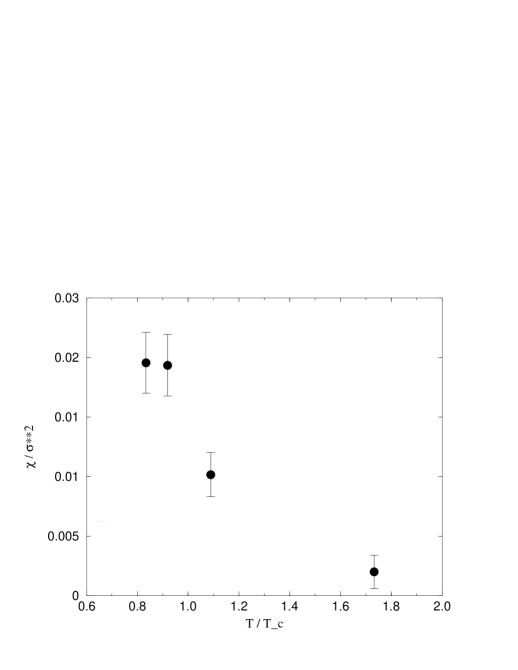
Figure 4: Topological susceptibility for inversely blocked configurations across the deconfining phase transition for Lüscher’s topological density

When the naive charges (that went into the susceptibility of smoothed configurations in Table 4) are multiplicatively corrected by the $Z_{q}^{(1)}(\beta)$ factors from Table 5 we get a unique $\beta$-dependence of $\chi_{top}$. We have shown in Fig. 4 the topological suceptibility for our four temperatures. The lattice spacing $a(\beta)$ has been non–perturbatively expressed through the zero temperature string tension as measured at each respective $\beta$–value on the $12^{4}$ lattice.

Assuming the value $\sigma=(440{\mathrm{M}eV})^{2}$ for the zero temperature string tension we estimate at $T=0.834~{}T_{c}$ a susceptibility $\chi_{top}=(165.5{\mathrm{M}eV})^{4}$. Compared with the standard value of $\chi_{top}=(180{\mathrm{M}eV})^{4}$ at zero temperature there is not much room for increase at smaller temperature.

Figure 5: Average topological activity $\langle A_{top}\rangle$ (according to Lüscher’s charge) of inversely blocked configurations as function of $T/T_{c}$

For building instanton models of vacuum structure it is important to know not only the topological susceptibility but also the average density of instantons and antiinstantons. Only in the most simple-minded dilute gas model the topological susceptibility coincides with this density. In addition to the total charge (eqs. (14) or (15)), the following operator is tentatively chosen to represent $N_{+}+N_{-}$, the number of instantons plus antiinstantons

$$A_{top}=\sum_{x}|q(x)|~{}~{}~{}.$$ (18)

We can understand this, somewhat loosely, as a measure for the temperature dependent average glueball field (gluon condensate). Let us call it ”topological activity”. Compared with measurements of this quantity on Monte Carlo configurations, it is reduced by $\frac{1}{25}$ to $\frac{1}{40}$ on inversely blocked configurations, depending on temperature. For normal Monte Carlo configurations there is too much noise at low values of $|q(x)|$. Without inverse blocking, $A_{top}$ is unreliable as an estimator of the number of instantons plus antiinstantons. In Fig. 5 we show the average topological activity of inversely blocked configurations as function of $T/T_{c}$. Between $\beta=1.54$ and $\beta=1.61$ (over temperatures from $T=0.92~{}T_{c}$ to $T=1.09~{}T_{c}$) it drops by $50$ per cent, but the decrease becomes slower at higher temperature.

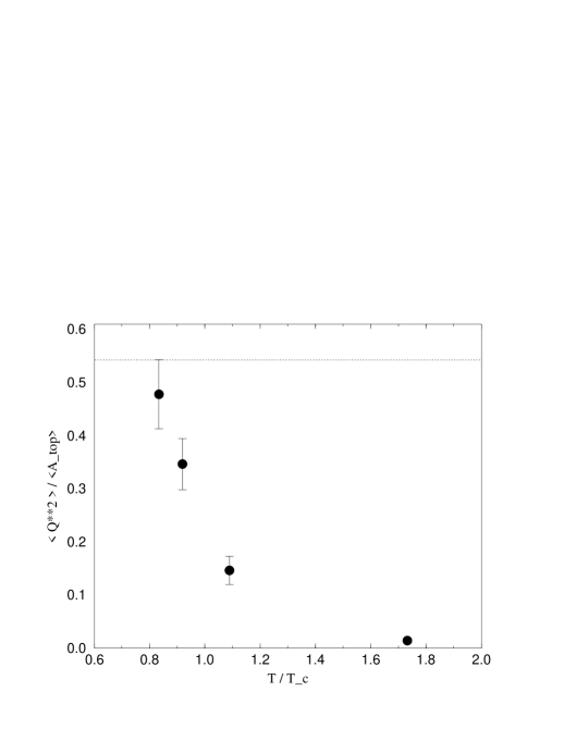
Figure 6: Ratio of topological susceptibility $\chi_{top}$ to average topological activity $\langle A_{top}\rangle/N_{sites}a^{4}$ (according to Lüscher’s charge) of inversely configurations as function of $T/T_{c}$

Concentrating now on the inversely blocked configurations, the topological susceptibility is strongly suppressed with increasing temperature, compared with the decrease of the topological activity. Fig. 6 demonstrates this additional suppression of uncompensated topological charge in the deconfinement phase. Apart from this observation, an interesting low temperature bound is suggested (see the dotted horizontal line in Fig. 6) :

$$\chi_{top}\leq\frac{6}{11}\frac{\langle A_{top}\rangle}{N_{sites}a^{4}}=\frac{6}{11}\langle n_{+}+n_{-}\rangle.$$ (19)

There is a factor $\frac{4}{b}=\frac{12}{11N_{c}}$ (equal to the entropic bound) in this relation where $b$ is the one–loop coefficient in the QCD $\beta$-function. Models describing this $O(1/N_{c})$ suppression of the topological susceptibility compared to the densities $n_{\pm}$ of instantons and antiinstantons have been discussed in an instanton liquid model with scale invariant hard core interaction [36] and in a similar droplet model [37].

We have found that (i) the topological susceptibility for smoothed configurations is of reasonable size on the confinement side of the transition, (ii) the topological susceptibility is smaller by a factor $\frac{4}{b}$ than the topological activity at low temperature and that (iii) the topological susceptibility decreases more than the topological activity entering the deconfinement phase.

4.2 Monopole Content of Monte Carlo and Inversely
Blocked Configurations

The Abelian monopole degrees of freedom are exposed by putting the lattice configurations into the maximally Abelian gauge [13]. Only few investigations have addressed the question how the dynamics of Abelian monopoles gets modified at the deconfinement transition and within the deconfined phase [12]. Abelian dominance is expected to become manifest at large distances. Hence it is natural to study these aspects in the ensemble of inversely blocked configurations which are smoothed at small distances.

It is not necessary to recall here details on the Abelian projection [13]. By a gauge cooling algorithm configurations are iteratively put into this gauge, whether they are directly Monte Carlo generated or obtained by inverse blocking. Finally, each configuration is mapped to a corresponding Abelian one. The links are represented by $U(1)$ phase factors and the non–diagonal fields are dropped. Using this new ensemble of configurations, confinement can be studied either in terms of Abelian Wilson loops formed out of the Abelianized links or, alternatively, in terms of the monopole currents. These are detected [14] seeking for magnetic flux penetrating the surface of a $3$-dimensional cube. Each time a non–zero flux is detected, the dual (with respect to the cube) link $x,\mu$ is said to carry a monopole current $m_{\mu}(x)$.

Figure 7: Ratio between the averages of total monopole current number $M$ and topological activity $A_{top}$ as function of $T/T_{c}$ for Monte Carlo and inversely blocked configurations

We do not discuss here the correct description of monopole condensation [38] and restrict ourselves to measurements of the monopole current numbers

$$M_{\mu}=\sum_{x}|m_{\mu}(x)|~{}~{}.$$ (20)

It is important to distinguish spacelike ($\mu=1,2,3$) and timelike ($\mu=4$) dual links carrying monopole currents. We will see that their numbers behave differently at the deconfinement temperature.

Figure 8: Ratio between the averages of timelike monopole current number $M_{t}$ and topological activity $A_{top}$ as function of $T/T_{c}$ for Monte Carlo and inversely blocked configurations

There are indications that the monopole current number $M=\sum_{\mu}M_{\mu}$ is related to the topological activity $A_{top}$. Both quantities are reduced by the same factor $\frac{1}{25}$ to $\frac{1}{40}$, at the lowest and the highest temperatures, respectively, as the result of blocking followed by inverse blocking. We show in Fig. 7 the ratio $\langle M\rangle/\langle A_{top}\rangle$. This ratio is a smoothly falling function of temperature across the phase transition for normal Monte Carlo configurations. For inversely blocked configurations, however, we find an sudden drop of this ratio at $T_{c}$. This is mainly due to the suppression of spatially directed monopole currents. The corresponding ratio for timelike monopole currents alone (see Fig. 8) is a smooth function of temperature for Monte Carlo and inversely blocked configurations.

The ratio between $M_{s}$ (summed over $\mu=1,2,3$) and $3~{}M_{t}$ ($\mu=4$) is expected to change at the deconfinement temperature [12]. In Fig. 9 the ratio $\langle M_{s}\rangle/3\langle M_{t}\rangle$ is shown for Monte Carlo and inversely blocked configurations as function of $T/T_{c}$. For the original Monte Carlo configurations the monopole current number is space–time symmetric in the confinement phase and the ratio $\langle M_{s}\rangle/3\langle M_{t}\rangle$ changes only slightly over the temperature range interpolating from the confinement to the deconfining phase. The deconfinement effect is not strong because it is hidden by the huge overall monopole activity in the Monte Carlo configurations. The effect becomes clear only for inversely blocked configurations.

Figure 9: Ratio between the averages of timelike and spacelike monopole currents across the deconfining phase transition for Monte Carlo and inversely blocked configurations

There exists an surplus of timelike monopole currents already in the confinement phase (which probably must be interpreted as a finite $L_{t}$ effect produced in the process of blocking). There is a strong reduction of spacelike monopoles at $T=1.089T_{c}$, and deeper in the deconfined phase they are completely suppressed.

Figure 10: $3$-dimensional densities of timelike and spacelike monopoles across the deconfining phase transition for inversely blocked configurations

Fig. 10 expresses the monopole currents for inversely blocked configurations in the form of $3$-dimensional densities

$$n_{\mu}=\frac{1}{N_{sites}a^{3}}~{}\langle M_{\mu}\rangle$$ (21)

of timelike and spacelike monopoles (in $\Lambda_{L}$ units) as a function of $T/T_{c}$. Monopoles, condensed in the confining phase, become static (massive) particle–like objects in the deconfined phase with a density rising with temperature (cf. Ref. [12] ). One may speculate about their relation to ’t Hooft–Polyakov monopoles. Spacelike monopole currents (responsible for confinement below $T_{c}$) become strongly suppressed at $T_{c}$ and have completely disappeared at $T\simeq 1.7~{}T_{c}$.

5 Resolving the Vacuum Structure

5.1 Topological Density Correlation

Information on the nature of topological excitations is contained

Figure 11: Normalized correlation function of the naive topological charge density at $\beta=1.5$ (for Monte Carlo and inversely blocked configurations) and at $\beta=1.8$ (only inversely blocked). Solid lines are fits according to eq. (22),(23)

in the point–to–point correlation function of the topological charge density. This is easy to measure, but for usual Monte Carlo configurations $U^{MC}$ this measurement has no value.

Several groups have attempted to define shape and size of topological excitations by the use of cooling techniques. The MIT group [31] has used for this purpose deeply cooled configurations. There is an uncertainty about the loss of essential structures during cooling. Sometimes there appears a particular structure just during the first few cooling steps [16, 24]. Recently, there have been attempts to improve cooling by choosing suitably improved actions [33, 34, 35] for (unconstrained) relaxation. Partial success has been achieved to stabilize instantons above some threshold in size. But certain topological structures (instanton-antiinstanton pairs) unavoidably disappear in the process of cooling. The method of inverse blocking is welcome because it enables to detect correlations on a set of well–defined configurations, which are smooth but interpolate, in a locally correct way, coarser equilibrium configurations.

In Fig. 11 we compare the normalized

Figure 12: Normalized correlation function of the geometric Lüscher topological charge density (as in Fig. 11)

correlation function of the topological charge density measured on the $12^{3}\times 4$ lattice in the confinement phase at $\beta=1.5$ on Monte Carlo and inversely blocked configurations. For normal Monte Carlo configurations there is no signal at any distance except for $x=0$. In order to demonstrate the influence of temperature on the signal we show in this figure also the correlation function measured at $\beta=1.8$ in the deconfinement phase. Due to the fixed normalization at $x=0$ only the change of the instanton radius can be seen (as explained below).

Smoothing is necessary in order to expose a signal in the density–density correlation function not only in the case of the naive topological density definition $q_{naive}(x)$. Fig. 12 shows the same for Lüscher’s charge density. The effect is similar, but the correlation of the naive charge density always extends somewhat farther. This can be understood due to the extended nature of the operator (13).

Getting a reasonable fit of the correlation function to the analytical shape derived from the instanton profile

$$q_{inst}(x)=\frac{6}{\pi^{2}\rho^{4}}\left(\frac{\rho^{2}}{x^{2}+\rho^{2}}\right)^{4}$$ (22)

by folding

$$\langle q(x)q(0)\rangle\propto\sum_{z}q_{inst}(x-z)q_{inst}(z),$$ (23)

we have determined the average instanton radii $\rho_{inst}$ as given in Table 6. The corresponding fitting curves are shown in Figs. 11 and 12. The instanton radius as determined by this method decreases more rapidly with rising temperature than the inverse temperature. Some change of $\rho_{inst}$ at deconfinement has been observed by the cooling method, too [39].

$\beta$	$1.50$	$1.54$	$1.61$	$1.80$
Lüscher’s charge	$1.4~{}a$	$1.4~{}a$	$1.35~{}a$	$1.1~{}a$
naive charge	$1.8~{}a$	$1.8~{}a$	$1.75~{}a$	$1.6~{}a$

Table 6: Instanton radii $\rho_{inst}$ in lattice units as estimated from the topological charge density correlation function at two $\beta$–values in the confinement and two $\beta$–values in the deconfinement phase, according to the two charge definitions

5.2 Monopole–Instanton Correlation

It has been demonstrated before for certain classical configurations that there is a close connection between instantons and monopole world loops. One can visualize this in the maximally Abelian gauge [15].

Figure 13: Normalized correlation function of monopole currents with topological charge density (according to Lüscher) at $\beta=1.5$ in the confinement phase

A nontrivial correlation has been measured between topological charge density and monopole currents in the Monte Carlo ensemble of Euclidean field configurations, too [16]. We show here in Fig. 13 the analogous normalized correlator for the original Monte Carlo ensemble (generated with the fixed point action at $\beta=1.5$ in the confinement phase) and for the corresponding ensemble of inversely blocked configurations. The latter correlator (for smoothed configurations) is slightly wider. In contrast to the topological density–density correlations, this correlator can be detected in the Monte Carlo configurations as well.

Comparing this with the same (normalized) correlation function at $\beta=1.8$ in the deconfined phase (not shown here), we find that they are identical as a function of the distance in lattice units within the error bars. This means that this correlation length changes proportional to the inverse temperature.

6 Conclusion and Outlook

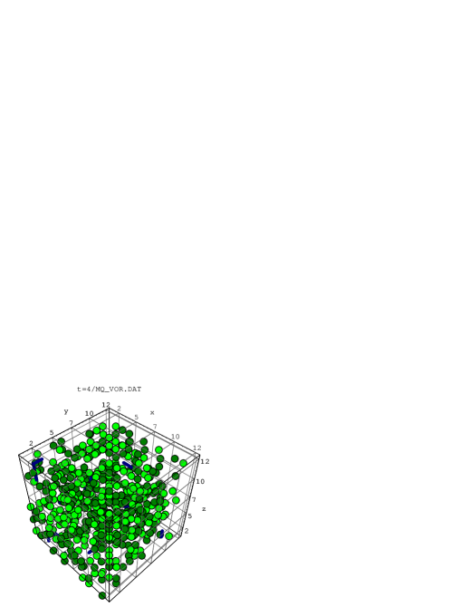
Figure 14: Lüscher’s topological charge density for $|q(x)|>q_{0}$ and monopole world lines in a timeslice of a typical Monte Carlo configuration in the confinement phase; signs of $q$ are distinguished by different color

We have explained in this paper how inverse blocking can be used to analyze topological structures of genuine quantum configurations, usually hidden under ultraviolet fluctuations.

Apart from cooling techniques, inverse blocking is the only way to measure autocorrelations of the topological density giving information on the size of instantons. Information on monopole currents is available also for normal Monte Carlo configurations. Monopoles are correlated with the topological density, both in Monte Carlo and inversely blocked configurations. However, the density of monopole currents is reduced, roughly proportional to the topological activity, if a configuration undergoes the procedure of blocking followed by inverse blocking.

Only a small part of Abelian monopoles seen usually in Monte Carlo configurations seems to be really important for confinement. This part survives smoothing in the confinement phase. We come to this conclusion because the string tension is found to be largely unaffected by the removal of ultraviolet fluctuations. This observation supports semiclassical scenarios of confinement. In the deconfinement phase, however, we find that spacelike monopoles are strongly suppressed for inversely blocked configurations while only timelike ones survive.

Armed with inverse blocking, we can do better than measuring the topological density–density correlation or the correlation between monopoles and topological density. We are now able to study clustering properties of the topological charge using inversely blocked lattice configurations. We can relate clusters of topological charge to the diluted network of monopole currents. Instead of examining idealized semiclassical configurations under different aspects of topological and monopole structure, the method of inverse blocking makes it possible to analyze generic Euclidean lattice field histories in order to characterize the physical phase one is dealing with. The results should be interesting for vacuum model builders. In view of chiral symmetry breaking and restoration, it would be also interesting to study the influence of the inverse blocking RG transformation on the spectrum of the Dirac operator.

The study of clusters of topological charge promises to give a more direct access to the parameters and correlations that should be built in an instanton model for QCD at zero and finite temperature. In Figs. 14 and 15 lattice hypercubes of one timeslice are marked if the Lüscher topological charge density exceeds a threshold

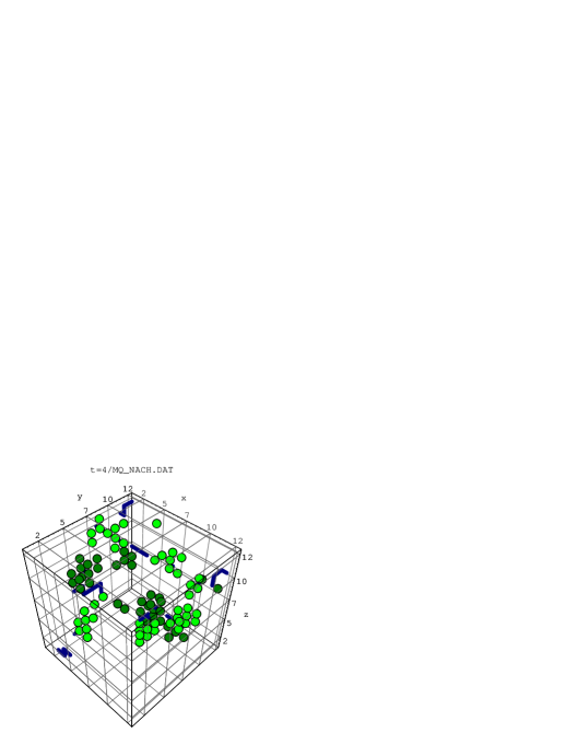
Figure 15: Clustering of the Lüscher topological charge density and monopole world lines in a timeslice of the same configuration as in Fig. 14 but after smoothing

value $q_{0}=0.015$. Different colors symbolize the sign. The original Monte Carlo configuration does not allow to guess any structure. The other picture shows the structure emerging after blocking and inverse blocking. The effect is the same using either naive or Lüscher’s charge density. Therefore one can abandon to use complicated algorithms and use naive or improved loop–oriented definitions of topological charge density.

There are two immediate directions for further studies.

• Study of the clustering properties of topological charge in individual lattice configurations and of the relation to the monopole currents.

• Repeating the present explorative study at higher $\beta$ with a particular emphasis on the scale dependence of topological structure.

Further progress in the construction of the perfect action should be incorporated into this program.

Note added:

During the time elapsed since the first submission of our article, several interesting papers have appeared which have attempted to investigate the space time topological structure of lattice gauge fields. Three methods have been used: (improved) cooling, fermionic (spectral) methods and smoothing. The latter method had been proposed in this paper as a general, renormalization group oriented pattern recognition method for large scale structures in terms of topological charge and monopoles which conserves the string tension.

While the subsequent studies were mostly focussed on vacuum (zero temperature) configurations, the results are still controversial as emphasized in Ref. [43]. As a generic rule, one can state that improved cooling [35] is biased towards larger instantons (because only those are stable) while the topological susceptibility tends to be lower; in contrast, the smoothing method (as developed further by the Boulder group [40]) favours smaller instanton sizes and tends to find somewhat higher topological susceptibility. This applies to $SU(2)$ pure gauge theory where the results can be compared (but not without additional assumptions).

We want to stress an important difference of Ref. [40] to the work published here. Smoothing has been applied there in an iterative way that leads finally to locally classical configurations. The number of iterations appears there as somewhat subjective parameter similar to the number of (unimproved or improved) cooling steps.

This goes far beyond our intention. From our point of view, the advantage of smoothing is that it provides a minimal smoothing of quantum fluctuations in clear correspondence to a certain scale. This scale is well–defined by the highest blocking level.

The effect of smoothing on various Abelian projections has been critically examined in Ref. [41]. The maximally Abelian gauge is the only one which seems to exhibit long range physics also if applied to smoothed lattice fields. While we had concentrated on the density of monopoles, it has been found there that the property of Abelian dominance (i.e. dominance of the Abelian string tension) is only partly preserved.

A large number of investigations was studying topological structures using fermionic methods going back to Smit and Vink [42]. It is important in the context of this work that these methods seem to work immediately, without smoothing or cooling techniques which otherwise would have to be applied to the Monte Carlo lattice gauge field configurations. Investigating the spectral flow of the lowest eigenvalues of the Dirac operator [43, 44, 45] these authors are able to count the number of localized lumps (and identify the respective sign) of topological charge. The local topological structure is thereby indirectly accessible through the localization properties of the corresponding eigenmodes. This has been checked in Refs. [45, 46] with cooling, but there is no comparison so far with the topological structure detected by smoothing.

We have recently improved our relaxation algorithm for implementing inverse blocking [47]. We are now in the position to optimize a fixed point action of moderate complexity for a given inverse blocking parameter $\kappa$. We could check a new parametrization of the perfect action for $SU(2)$ which is truncated compared with the action used in Ref. [40]. We thank the Boulder group for correspondence about that and for providing the truncated action [48]. We can now show that the parametrization of Table 1 is not compatible with the $\kappa=12$ required. This inconsistency had forced us to accept (in this paper) a smaller effective $\kappa$. We have convinced ourselves that the statistical observations are independent of this choice although the inversely blocked configurations may differ locally.

References

- [1] C. G. Callan, R. Dashen and D. J. Gross, Phys. Rev. D 17, (1978) 2717; D. J. Gross, R. D. Pisarski and L. G. Yaffe, Rev. Mod. Phys. 53, (1981) 43
- [2] E. Shuryak, Phys. Reports 264, (1996) 357; T. Schäfer and E. V. Shuryak Phys. Rev. D 54, (1996) 1099; T. Schäfer and E. V. Shuryak, Phys. Rev. D 53, (1996) 6522; T. Schäfer and E. V. Shuryak, e-print archive hep-ph/9610451
- [3] S. Mandelstam, Phys. Reports 23C, (1976) 245
- [4] G. ’t Hooft, Nucl. Phys. B 190, (1981) 455
- [5] F. Niedermayer, Nucl. Phys. B Proc. Suppl. 53 (1997) 56; W. Bietenholz, R. Brower, S. Chandrasekharan and U. J. Wiese, Nucl. Phys. B Proc. Suppl. 53 (1997) 921
- [6] T. A. DeGrand, A. Hasenfratz, P. Hasenfratz, F. Niedermayer, and U. J. Wiese, Nucl. Phys. B Proc. Suppl. 42 (1995) 67; T. DeGrand, A. Hasenfratz, P. Hasenfratz and F. Niedermayer, Nucl. Phys. B 454, (1995) 587; Nucl. Phys. B 454, (1995) 615; Phys. Lett. B 365, (1996) 233; M. Blatter and F. Niedermayer, Nucl. Phys. B 482, (1996) 286
- [7] T. DeGrand, A. Hasenfratz, P. Hasenfratz, P. Kunszt and F. Niedermayer, Nucl. Phys. B Proc. Suppl. 53 (1997) 942
- [8] T. DeGrand, A. Hasenfratz and De-cai Zhu, Nucl. Phys. B 475, (1996) 321
- [9] T. DeGrand, A. Hasenfratz and De-cai Zhu, Nucl. Phys. B 478, (1996) 349
- [10] E.–M. Ilgenfritz, M. L. Laursen, M. Müller–Preussker, G. Schierholz and H. Schiller, Nucl. Phys. B 168, (1986) 693; M. Teper, Phys. Lett. B 162, (1985) 357
- [11] V. G. Bornyakov, E.–M. Ilgenfritz, M. L. Laursen, V. K. Mitrjushkin, M. Müller–Preussker and A. J. van der Sijs, Phys. Lett. B 261 (1991) 116
- [12] V. G. Bornyakov, V. K. Mitrjushkin and M. Müller-Preussker, Phys. Lett. B 284, (1992) 99
- [13] A. S. Kronfeld, G. Schierholz and U. J. Wiese, Nucl. Phys. B 293, (1987) 461; A. S. Kronfeld, M. L. Laursen, G. Schierholz and U. J. Wiese, Phys. Lett. B 198, (1987) 516
- [14] T. A. DeGrand and D. Toussaint, Phys. Rev. D 22, (1980) 2478
- [15] V. G. Bornyakov and G. Schierholz, Phys. Lett. B 384, (1996) 190; M. N. Chernodub and F. V. Gubarev, JETP Lett. 62, (1995) 100; A. Hart and M. Teper, Phys. Lett. B 371, (1996) 261; R. C. Brower, K. N. Orginos and C.–I Tan, Nucl. Phys. B Proc. Suppl. 53 (1997) 488 and e-print archive hep-th/9610101
- [16] S. Thurner, M. Feurstein, H. Markum and W. Sakuler, Phys. Rev. D 54, (1996) 3457; S. Thurner, H. Markum and W. Sakuler, in Proceedings of Confinement 95, Osaka 1995, eds. H. Toki et al. (World Scientific, 1996) 77; H. Markum, W. Sakuler and S. Thurner, Nucl. Phys. B Proc. Suppl. 47 (1996) 254
- [17] A. Phillips and D. Stone, Comm. Math. Phys. 103, (1986) 599; A. S. Kronfeld, M. L. Laursen, G. Schierholz, C. Schleiermacher and U. J. Wiese, Comp. Phys. Comm. 54, (1989) 109
- [18] M. Lüscher, Comm. Math. Phys. 85, (1982) 29
- [19] I. A. Fox, J. P. Gilchrist, M. L. Laursen and G. Schierholz, Phys. Rev. Lett. 54, (1985) 749; A. S. Kronfeld, M. L. Laursen, G. Schierholz and U. J. Wiese, Nucl. Phys. B 292, (1987) 330
- [20] P. Di Vecchia, K. Fabricius, G. C. Rossi and G. Veneziano, Nucl. Phys. B 192, (1981) 392; Phys. Lett. B 108, (1982) 323; Phys. Lett. B 249, (1990) 490
- [21] N. V. Makhaldiani and M. Müller–Preussker, JETF Pisma 37, (1983) 440
- [22] M. Göckeler, A. S. Kronfeld, M. L. Laursen, G. Schierholz and U. J. Wiese, Phys. Lett. B 233, (1989) 192
- [23] A. Di Giacomo, E. Meggiolaro and H. Panagopoulos, Phys. Lett. B 277, (1992) 491
- [24] E.–M. Ilgenfritz, E. Meggiolaro and M. Müller–Preussker, Nucl. Phys. B Proc. Suppl. 42 (1995) 496
- [25] C. Christou, A. Di Giacomo, H. Panagopoulos and E. Vicari, Phys. Rev. D 53, (1996) 2619
- [26] B. Alles, M. D’Elia and A. Di Giacomo, Nucl. Phys. B Proc. Suppl. 53 (1997) 541 and e-print archive 9605013
- [27] see the second of Ref. [6]
- [28] M. Falcioni, M. Paciello, G. Parisi and B. Taglienti, Nucl. Phys. B 251, (1985) 624; M. Albanese et al., Phys. Lett. B 192, (1987) 163
- [29] M. Campostrini, A. Di Giacomo, M. Maggiore H. Panagopoulos and E. Vicari, Phys. Lett. B 225, (1989) 403
- [30] M. Campostrini, A. Di Giacomo and H. Panagopoulos, Phys. Lett. B 212, (1988) 206; M. Campostrini, A. Di Giacomo, H. Panagopoulos and E. Vicari, Nucl. Phys. B 329, (1990) 683
- [31] M. C. Chu, J. M. Grandy, S. Huang and J. W. Negele, Phys. Rev. D 49, (1994) 6039; R. C. Brower, T. L. Ivanenko, J. W. Negele and K. N. Orginos, Nucl. Phys. B Proc. Suppl. 53 (1997) 547
- [32] A. Di Giacomo and E. Vicari, Phys. Lett. B 275, (1992) 429; B. Alles, M. Campostrini, A. Di Giacomo, Y. Gündüc and E. Vicari, Phys. Rev. D 48, (1993) 2284
- [33] M. Garcia Perez, A. Gonzalez–Arroyo, J. Snippe and P. van Baal, Nucl. Phys. B 413 (1994) 535
- [34] P. de Forcrand, M. Garcia Perez and I.–O. Stamatescu, Nucl. Phys. B Proc. Suppl. 47 (1996) 278 and 777
- [35] P. de Forcrand, M. Garcia Perez and I.–O. Stamatescu, Nucl. Phys. B 499 (1997) 409; P. de Forcrand, M. Garcia Perez, J. E. Hetrick and I.–O. Stamatescu, contribution to Lattice 97, e-print archive hep-lat/9710001
- [36] E.–M. Ilgenfritz and M. Müller–Preussker, Phys. Lett. B 99, (1981) 128
- [37] G. Münster, Z. f. Phys. C 12, (1982) 43
- [38] L. Del Debbio, A. Di Giacomo, G. Paffuti and P. Pieri, Nucl. Phys. B Proc. Suppl. 42 (1995) 234 and Phys. Lett. B 355, (1995) 255; M. N. Chernodub, M. I. Polikarpov and A. I. Veselov, Nucl. Phys. B Proc. Suppl. 49 (1996) 307 and e-print archive hep-lat/9610007; A. I. Veselov, M. I. Polikarpov and M. N. Chernodub, JETP Lett. 63, (1996) 411
- [39] M. C. Chu and S. Schramm, Phys. Rev. D 51, (1995) 4580
- [40] T. DeGrand, A. Hasenfratz, T. G. Kovacs, e-print archive hep-lat/9705009; and contribution to Lattice 97, e-print archive hep-lat/9709095
- [41] T. G. Kovacs, Z. Schram, e-print archive hep-lat/9706012, Phys. Rev. D (to be published)
- [42] J. Smit and J. Vink, Nucl. Phys. B 286, (1987) 485, B 303, (1988) 36
- [43] R. Narayanan and R. L. Singleton, contribution to Lattice 97, e-print archive hep-lat/9709014
- [44] R. Narayanan and P. Vranas, e-print archive hep-lat/9702005, Nucl. Phys. B (to be published)
- [45] D. Smith, H. Simma and M. Teper (UKQCD Collaboration), contribution to Lattice 97, e-print archive hep-lat/9709128
- [46] T. L. Ivanenko and J. W. Negele, contribution to Lattice 97, e-print archive hep-lat/9709130; J. W. Negele, contribution to Lattice 97, e-print archive hep-lat/9709129
- [47] E.–M. Ilgenfritz, M. Müller–Preussker and S. Thurner, in progress
- [48] T. G. Kovacs, private communication