Continuum limit of finite temperature $\lambda\phi^{4}_{3}$ from lattice Monte Carlo.

Abstract

The $\phi^{4}_{3}$ model at finite temperature is simulated on the lattice. For fixed $N_{t}$ we compute the transition line for $N_{s}\to\infty$ by means of Finite Size Scaling techniques. The crossings of a Renormalization Group trajectory with the transition lines of increasing $N_{t}$ give a well defined limit for the critical temperature in the continuum. By considering different RG trajectories, we compute $T^{c}/g$ as a function of the renormalized parameters.

DFTUZ/96/21 DSF 96/50 hep-lat/9610038

1 Introduction

Finite temperature phase transitions in Relativistic Quantum Field Theories have been the subject of an intense study since the time of the pioneering work of Kirzhnitz and Linde [1], Weinberg [2] and Dolan and Jackiw [3], which revealed that, in general, spontaneously broken symmetries get restored above a certain critical temperature $T^{c}$ . While the nature of this phenomenon is by now well understood, an accurate description of the transition, including sometimes its order, as well as a precise determination of the critical temperature can be difficult because of the appearance, at the transition point, of infrared divergencies which cause the breakdown of ordinary perturbation theory [3]. Even though new analytic non-perturbative methods, allegedly immune of infrared problems, have recently been developed and have been used to attack this sort of problems [6], the failure of the standard analytic methods has motivated some authors to study these phase transitions on computers and these days massive simulations of the electroweak phase transition are being performed (see for example [7]).

In this paper we report on the results of a lattice Monte Carlo simulation of the $\lambda\phi^{4}_{3}$ theory at finite temperature. There are definite reasons to be interested in this simple system. First of all it is believed that the $\phi^{4}_{3}$ theory admits a non-trivial continuum limit (at $T=0$) [8, 9, 10, 11, 12], contrary to $\phi^{4}_{4}$. Moreover, $\phi^{4}_{3}$ is superrenormalizable [13], so that primitive ultraviolet divergences occur only in a finite number of diagrams, and this allows one to exactly compute its $\beta$ functions. The model is expected to undergo a second order phase transition at a finite critical temperature but despite its simple ultraviolet properties, its behavior near the transition is particularly hard to explore, because infrared divergencies get worsened in three dimensions and as a matter of fact there is no reliable way of computing the critical temperature in perturbation theory, not even to lowest order [14]. Finite Temperature Renormalization Group methods may nevertheless be used to get estimates of the critical temperature [15].

It appears natural to see if better results can be obtained from the lattice. In this respect, there exist theorems proving that on the lattice spontaneously broken symmetries get always restored at sufficiently high temperatures (in an arbitrary number of dimensions) [16, 17]. Unfortunatly, these theorems only provide upper bounds on the critical temperature (for finite lattice spacings), which cannot be used to determine the critical temperature in the continuum limit, not being strong enough to even guarantee that the critical temperature remains finite when the lattice spacing is taken to zero.

Of the existing lattice studies of the $\phi^{4}_{3}$-theory at finite temperature, some combine approximate analytical treatments with numerical work to get estimates of the critical temperature in the continuum limit [18, 19], while others use a Monte Carlo simulation [20]. This paper represents a significant improvement and extension of these results. We have carried out a Monte Carlo simulation on large lattices with massive statistics, making a detailed study of finite size effects and of the continuum limit.

Within the path integral formalism, finite temperature is introduced by compactifying the euclidean time direction, temperature being the inverse of the temporal extension [21]. When doing simulations on the lattice, this goal is achieved by using asymmetric lattices $N_{t}\times{N_{s}}^{2}$ shorter in the temporal direction. However, in order to avoid finite size effects and approach the continuum limit, these steps should be followed:

1. For a finite $N_{t}$ take the limit $N_{s}\to\infty$.

2. Take the lattice spacing $a$ to 0 and $N_{t}$ to $\infty$.

Our aim is to measure the critical temperature for which symmetry restoration arises. For fixed $N_{t}$ we have computed, for several values of $N_{s}$, the transition line that separates the broken and symmetric phases. By means of Finite Size Scaling (FSS) techniques we have obtained the line for $N_{s}\to\infty$. We have done this for several values of $N_{t}$. When increasing $N_{t}$, the transition lines approach that of zero temperature. These critical lines have been used to measure $T^{c}$ in the following way. A possible continuum theory is defined by a “curve of constant physics” (CCP): it is parametrised by the lattice spacing $a$ and, as $a\rightarrow 0$, it approaches the critical line of the symmetric lattice. While doing so, it intersects the critical lines of the lattices with finite $N_{t}$. Each intersection point gives a critical temperature, $T_{N_{t}}=\frac{1}{N_{t}a}$, and $T^{c}$ is just the limit (if it exists) of all these temperatures.

Due to the super-renormalizability of the model, the asymptotic form of the CCP’s that approach the gaussian fixed point can be computed exactly in perturbation theory. We have considered several CCP’s and have accepted only those for which the correlation length, measured numerically, has shown a satisfactory scaling. For these trajectories we have found a well defined limit for the critical temperatures and we have been able to verify the relation predicted in [15] between $T^{c}$ and the renormalized parameters of the continuum model (defined using dimensional regularization in the Minimal Subtraction (MS) scheme)

$$T^{c}\log\left(\frac{4\pi kT^{c}}{g}\right)=-\frac{8\pi m^{2}_{MS}(T^{c})}{g}~{},$$ (1)

where $m_{MS}(T^{c})$ is the value of the running mass at the scale $T^{c}$, $g$ is the coupling constant and $k$ is a factor not calculable perturbatively. We have obtained an estimate of $k=2.1(2)$.

The plan of the paper is as follows. In Sec.2 we present the model. Sec.3 defines the curves of constant physics. In Sec.4 we discuss the effects of a finite temperature and explain how to measure its critical value. Sec.5 describes the details of the Monte Carlo simulation and the observables that have been measured. The results are presented in Sec.6. Finally, Sec.7 is devoted to the conclusions.

2 The $\lambda\phi^{4}_{3}$ model

We consider the theory for a real scalar field in 3 euclidean dimensions, described by the bare (euclidean) action:

$$S=\int d^{3}x\left[\frac{1}{2}(\partial_{i}\Phi_{B})^{2}+\frac{1}{2}m^{2}_{B}\Phi_{B}^{2}+\frac{g_{B}}{4!}\Phi^{4}_{B}\right]~{}~{}.$$ (2)

When regularized on an infinite three-dimensional cubic lattice of points $\Omega$ with lattice spacing $a$, the above action is replaced by the discretized expression:

$$S_{L}=\sum_{x\in\Omega}a^{3}\left\{\frac{1}{2}\sum_{\mu}(\Delta^{(a)}_{\mu}\Phi_{L})^{2}(x)+\frac{1}{2}m^{2}_{B}\Phi_{L}^{2}(x)+\frac{g_{B}}{4!}\Phi^{4}_{L}(x)\right\}~{}~{}$$ (3)

where $\Delta^{(a)}_{\mu}$ is the lattice derivative operator in the direction $\mu$

$$\Delta^{(a)}_{\mu}\Phi_{L}(x)\equiv\frac{\Phi_{L}(x+\hat{\mu}a)-\Phi_{L}(x)}{a}~{}~{}.$$

It is convenient to measure all quantities in the action (3) in units of the lattice spacing. We thus define:

$$\phi_{L}(x)\equiv a^{1/2}\Phi_{L}(x),~{}~{}~{}u\equiv ag_{B},~{}~{}~{}r\equiv a^{2}m^{2}_{B}~{}~{}.$$ (4)

In terms of the rescaled quantities the action now reads:

$$S_{L}=\sum_{x\in\Omega}\left\{\frac{1}{2}\sum_{\mu}(\Delta_{\mu}^{(1)}\phi_{L})^{2}(x)+\frac{1}{2}r\phi_{L}^{2}(x)+\frac{u}{4!}\phi_{L}^{4}(x)\right\}~{}~{}.$$ (5)

In order to conform with the customary lattice notation, we perform a further redefinition of the field and parameters in (5):

$$\phi_{L}(x)\equiv{\sqrt{\kappa}}\phi_{\mbox{\scriptsize\boldmath$r$}},~{}~{}~{}u=\frac{24\lambda}{\kappa^{2}},~{}~{}~{}r=2\frac{1-2\lambda-3\kappa}{\kappa}~{}~{}$$ (6)

and thus write the action in our final form:

$$S_{L}=\sum_{\mbox{\scriptsize\boldmath$r$}\in{\bf Z^{3}}}\left\{-\kappa\sum_{\mu}\phi_{\mbox{\scriptsize\boldmath$r$}}\phi_{\mbox{\scriptsize\boldmath$r$}+\hat{\mbox{\scriptsize\boldmath$\mu$}}}+\lambda(\phi^{2}_{\mbox{\scriptsize\boldmath$r$}}-1)^{2}+\phi^{2}_{\mbox{\scriptsize\boldmath$r$}}\right\}\ .$$ (7)

This model has been intensely studied at zero temperature, using renormalization group and high temperature expansion techniques [10], and also numerically [8, 9, 11, 12], and its features are well known. As it is apparent from the action, it has a $Z_{2}$ symmetry which can be spontaneously broken, if the double-well potential is deep enough. In the parameter space $(\kappa,\lambda)$ there exist two fixed points: one is the gaussian fixed point $(\kappa=1/3,\lambda=0)$ while the other is in the same universality class as that of the 3d Ising model. The gaussian fixed point has a null attraction domain and the whole transition line (except just the origin) possesses the Ising critical exponents.

3 The Curves of Constant Physics

In this section we define the CCP’s which define the continuum limit of our lattice model. They are Renormalization Group trajectories of the theory at zero temperature.

Suppose we start from a symmetric $N^{3}$ lattice with spacing $a_{0}$ and bare parameters $m^{2}_{B},~{}g_{B}$. In order to take the continuum limit, we have to vary $a$ in the interval $[a_{0},0)$ and simultaneously adjust the values of $m^{2}_{B},~{}g_{B}$, in such a way that physical observables approach a constant value when $a\rightarrow 0$. If there were no need for renormalization, this would be a trivial task: it would suffice to hold $m^{2}_{B}$ and $g_{B}$ constant in eq.(4) and this would tell us how to adjust the dimensionless lattice parameters $u$ and $r$ with $a$ in the approach to the continuum. Unfortunatly, things are not so easy and the above procedure would fail, for example, to produce in the continuum a finite physical mass for the lightest boson. Because of the interaction, it is necessary to give the lattice parameters a non trivial dependence on $a$ in order for the observables, like the masses, to approach a finite limit for $a\rightarrow 0$ and we call “curves of constant physics” (CCP’s) any dependence of the lattice parameters $(u,r)$ (or equivalently $(\kappa,\lambda)$) on $a$ which achieves this goal.

In principle, a possible way of defining the CCP’s would be by requiring that two observables $({\cal O}_{1},{\cal O}_{2})$, constructed out of the Green’s functions of the theory (for example the physical mass of the boson and the coupling constant at some fixed momentum scale), keep a constant value in physical units when $a$ is varied. The CCP will depend of course on the choice of $({\cal O}_{1},{\cal O}_{2})$, but for $a$ sufficiently small they will all coincide and define the same continuum physics, possibly parametrized in different manners.

As from a numerical point of view this strategy is very hard to implement, we have utilized a different procedure to construct our CCP, based on the fact that our model is perturbatively super-renormalizable. Due to this property, the perturbative expansion of the theory contains only a finite number of ultraviolet primitively divergent diagrams [13]. Concretely, depending on the regularization scheme, such divergencies can occur only in the one-loop “tadpole” diagram and in the two-loop “sunset” diagram, and both can be reabsorbed via a redefinition of the mass term. As a consequence, no infinite renormalization of the field and of the coupling constant are needed and we can thus identify the bare field $\Phi_{B}$ and the bare coupling $g_{B}$ in (2) with the renormalized ones, $\Phi_{R}$ and $g_{R}$, respectively. We can then rewrite the action (2) as:

$$S=\int d^{3}x\left[\frac{1}{2}(\partial_{i}\Phi_{R})^{2}+\frac{1}{2}m^{2}_{B}\Phi_{R}^{2}+\frac{g_{R}}{4!}\Phi^{4}_{R}\right]~{}~{}.$$ (8)

(From now on we shall omit writing the subscript $R$ of all renormalised quantities, for simplicity.) In this expression, the only divergent quantity is thus $m^{2}_{B}$. We split it as:

$$m^{2}_{B}=m^{2}+\delta m^{2}$$ (9)

where $m^{2}$ represents the tree level mass term and $\delta m^{2}$ is a mass-counterterm which diverges in the limit $a\rightarrow 0$. The expression of $\delta m^{2}$ depends of course on the renormalization scheme. Its computation becomes especially easy in the lattice analogue of the minimal subtraction scheme, because all is needed then are the divergent parts of the lattice tadpole and sunset diagrams. All the formulae needed for this computation can be found, for example, in [7] and here we just quote the answer (for the limit $N\rightarrow\infty$):

$$m^{2}_{B}=m^{2}(\mu)-\frac{\Sigma}{8\pi a}g-\frac{1}{96\pi^{2}}g^{2}\ln(a\mu)~{},$$ (10)

where $\mu$ is an arbitrary mass scale and $\Sigma=3.1759114$.

With the above expression for the bare mass, the perturbative expansion of the Green’s functions of the theory is finite to all orders and thus all the observables that can be constructed out of them have a well defined limit for $a\rightarrow 0$. This suggests that we define as CCP those that simply have a fixed value of $m^{2}$ (at some fixed scale $\mu$) and of $g$. A similar approach was used and shown to work properly for 2d $\lambda\phi^{4}$ [22].

Using eq. (10) and the definition of the lattice parameters eq.(4), it is easy to see that the CCP, starting from some initial point $a_{0}$, $r_{0}$ (at the scale $\mu_{0}$), $u_{0}$, takes then the form

$$u(s)=su_{0}~{},$$

$$r(s)=s^{2}\left(r_{0}+\frac{\Sigma}{8\pi}u_{0}\left(1-\frac{1}{s}\right)-\frac{1}{96\pi^{2}}u_{0}^{2}\ln s\right)~{},$$ (11)

where $s=a/a_{0}$. Notice that, according to these formulae, the CCP’s approach the gaussian fixed point, as it must be having been computed within perturbation theory.

The parameters $m^{2}$ and $g$ just represent renormalised quantities and do not constitute a pair of observables that can be measured directly on the lattice. Consider instead one such observable, for example the physical mass of the lightest particle, $m_{phys}$, which is simply related to the correlation length at large separations $\xi_{phys}$, since $m_{phys}=\xi_{phys}^{-1}$. Now, when computed in perturbation theory starting from (8), with $m^{2}_{B}$ given by (10), $m_{phys}^{2}$ becomes a function of $m^{2},~{}g$ and $a$, admitting a finite limit for $a\rightarrow 0$. On dimensional grounds we can write this function as

$$m_{phys}^{2}=m^{2}F(g/m,am).$$

When the continuum limit is sufficiently near, the dependence on $a$ of the r.h.s. becomes negligible, $m_{phys}$ and thus the correlation length $\xi_{phys}$ become independent on $a$ and this implies that the lattice correlation length $\xi=\xi_{phys}/a$ becomes proportional to $1/a$.

In terms of the parameter $s$ introduced earlier, the region of continuum physics, along the CCP, is that for which the lattice correlation length scales according to

$$\xi(s)\propto\frac{1}{s}~{}.$$ (12)

Moreover, one should always have $\xi>1$ in order for the lattice details to be irrelevant and $\xi<N$ in order for finite size effects to be negligible.

4 Finite temperature

We briefly discuss the effects of a finite temperature on our system and how to measure $T^{c}$ on the lattice.

Let us suppose that the system is in the ordered phase at $T=0$ and imagine heating it up. The intuitive picture, valid in general, is that disorder increases, as the temperature is raised, until one reaches a critical value $T^{c}$ above which no order is possible any more and the full symmetry of the lagrangian is restored. This simple picture is confirmed by analytical treatments in four space time dimensions [2, 3].

In three dimensions things are less simple. Consider our $\phi^{4}_{3}$ model: while the existence of the symmetry restoring phase transition at a finite temperature seems sure, a reliable perturbative computation of the critical temperature, using standard techniques, is problematic due to the presence of severe infrared divergencies. For example, when taking a high temperature expansion of the one-loop effective potential one finds that the leading field-dependent term becomes complex for small fields, and this leads to a physically unacceptable complex value for the critical temperature. The situation does not improve upon resumming the so called daisy and super-daisy diagrams [3]: the resulting gap equation determining the thermal mass becomes meaningless at the critical temperature [14].

To our knowledge, the best analytical estimate of $T^{c}$ for the $\phi^{4}_{3}$ model is the one recently obtained in [15] using renormalization group methods. It is given in terms of an implicit equation for $T^{c}$:

$$\frac{T^{c}}{g}\log\left(\frac{4\pi kT^{c}}{g}\right)=-\frac{8\pi m^{2}_{MS}(T^{c})}{g^{2}}~{},$$ (13)

where $m^{2}_{MS}(\mu)$ is the running mass

$$m^{2}_{MS}(\mu)=m^{2}_{MS}(\mu_{1})+\frac{g^{2}}{96\pi^{2}}\log\left(\frac{\mu}{\mu_{1}}\right)~{}.$$ (14)

According to [15], the uncertainty on the value of $T^{c}$ due to the breakdown of perturbation theory in the vicinity of the phase transition only affects the value of the number $k$ in eq.(13). It cannot be computed analytically but is expected to be of order one and, as will be shown later, we have been able to measure it quite accurately.

The difficulties on the analytical side motivated us to study the phase transition of $\phi^{4}_{3}$ on the lattice. In order to simulate a finite physical temperature we work on an $N_{t}\times{N_{s}}^{2}$ lattice. For every $N_{t}$ considered, we have performed a series of simulations for several values of $N_{s}$, and using FSS techniques we have obtained the transition line in the thermodynamic limit $N_{t}\times{\infty}^{2}$. Repeating this analysis for different values of $N_{t}$ we have obtained several transition lines. For decreasing $N_{t}$ the critical lines shift deeper inside the broken region of the symmetric lattice, though all of them meet at the gaussian fixed point ($\kappa=1/3,\lambda=0$) whenever $N_{t}>1$.

Consider now a CCP, call it $\gamma$, lying in the ordered region of the $T=0$ theory and let $P$ be its starting point. Since the critical lines for finite $N_{t}$ approach, in the limit $N_{t}\rightarrow\infty$, that of the $T=0$ theory, $P$ will also lie in the ordered regions of the lattices with finite $N_{t}$, for $N_{t}$ large enough (how large it depends on $P$, of course). Choose now one such $N_{t}$, and imagine moving along the CCP. In this process $a$ diminishes and thus the physical temperature associated with the $N_{t}$ chosen grows up since $T=1/N_{t}a$. At some point our CCP will cross the transition line for this value of $N_{t}$ and symmetry will be restored. If $a_{N_{t}}$ is the value of the lattice spacing along the CCP at the crossing point, we have an estimate of the critical temperature:

$$T_{N_{t}}=\frac{1}{N_{t}a_{N_{t}}}$$ (15)

In order to get the continuum critical temperature we have to let $N_{t}\rightarrow\infty$. When $N_{t}$ is increased, the corresponding critical line gets closer to that of the $T=0$ theory and $\gamma$ will intersect it for a smaller value of $a$. The temperatures $T_{N_{t}}$ are thus expected to approach a limit, which is the desired continuum critical temperature $T^{c}$ for the continuum theory associated with $\gamma$.

In the absence of an external input which fixes the energy scale, we can assign a value $a=a_{0}$ to an arbitrary point on the CCP and then the value of $a$ at any other point on the trajectory is given by equations (11). In this way we can compare the temperatures $T_{N_{t}}$ corresponding to different values of $N_{t}$ for a given CCP, but it is not possible to put together the values from distinct CCP’s due to the arbitrariness in the scale. To avoid this problem, one can measure adimensional quantities, obtained for instance from the quotient of two observables with the same dimensions. Of this sort are the quantities $T^{c}/g$ and ${m^{2}_{MS}}(T^{c})/g^{2}$ entering equation (13).

The analysis of [15] was carried in the continuum, using dimensional regularization and minimal subtraction, while we are using the lattice regularization. So, in order to compare the results of our simulations with eq.(13), we have to first relate the continuum renormalized parameters appearing in eq.(13) to ours. In view of what we said earlier about the ultraviolet properties of the model, the only non trivial relation that needs to be computed is the one among the mass parameters of the two schemes. Using the formulae of [7] for the relevant two-loops diagrams contributing to the self-energy, it is not hard to check that:

$$m^{2}_{MS}(\mu)=m^{2}(\mu)-\frac{g^{2}}{96\pi^{2}}(\log 6+\zeta)+o(g^{3})~{},$$ (16)

where $\zeta=0.09$ and $m^{2}(\mu)$ is the lattice renormalized mass defined in eq.(10). Upon using eqs.(10), (16) and (15), we can now relate the adimensional quantities $T^{c}/g$ and ${m^{2}_{MS}}(T^{c})/g^{2}$ to the simulation parameters according to the following equations:

$$\frac{{m^{2}_{MS}}(T^{c})}{g^{2}}=\lim_{N_{t}\rightarrow\infty}\frac{1}{u^{2}}\left(r+\frac{\Sigma}{8\pi}u-\frac{1}{96\pi^{2}}u^{2}(\log N_{t}+\log 6+\zeta)\right),$$ (17)

$$\frac{T^{c}}{g}=\lim_{N_{t}\rightarrow\infty}\frac{1}{N_{t}u}$$ (18)

where $u$ and $r$ are evaluated at the points in which the CCP intercepts the critical line of the $N_{t}$-lattice. In our simulation we have measured the above quantities for various CCP’s, and this allowed us to check the validity of eq.(13) and measure, at the same time, the value of the unknown parameter $k$.

5 Monte Carlo simulation and observables

In the course of the simulations, most of our efforts went into the computation of the critical lines for different values of $N_{t}$. On the other hand, we have made measurements also on the symmetric lattice in order to identify the scaling region of our perturbative CCP’s.

We have used a Metropolis algorithm combined with a Wolff single cluster method [23] (the latter updates the sign of the field), taking a ratio of 20 clusters every 3 Metropolis iterations or 10 clusters every 2 Metropolis. These values are inside the region of ratios we have found nearly optimal for decorrelation versus CPU time close to the critical lines. When, in the intent of checking the CCP’s, we have measured the correlation lengths on the symmetric lattices, the simulations have been performed in the ordered region of the phase diagram and there the clustering is not so effective. However these simulation points did not lie very deep in the broken phase and then we have used this method as well.

The most intensive simulations have been those relative to the asymmetric lattices. We have used four different values of $N_{t}$ $(2,3,4,6)$ and for each of them we have computed the critical value of $\kappa$ for four values of $\lambda$ ($0.0005$, $0.001$, $0.002$, $0.003$). For each pair $(N_{t},\lambda)$, we have considered lattices of $N_{s}=12,16,24,32$, performing on each of them a single simulation for one value of $\kappa$. This value has been chosen near the critical one, by means of an hysteresis or by extrapolating from the values found for the previous lattices. Afterwards, we have used the spectral density method (SDM) [24] to extrapolate the measurements to other values of $\kappa$ in the vicinity of the simulation point. Finally, the value of $\kappa$-critical in the limit $N_{s}\to\infty$ has been computed by examining the crossings of the Binder cumulants relative to lattices with different values of $N_{s}$, as explained below.

At each of the points and lattices that have been simulated, the number of iterations made has been approximately $1,500,000\times(3~{}Metropolis+20~{}Clusters)$ or $2,500,000\times(2~{}Metropolis+10~{}Clusters)$, for a total CPU time equivalent to nearly one year of workstation. Most of the simulations have been carried out with iterations consisting of $3~{}Metropolis+20~{}Clusters$ and performing measurements only at intervals of 10 iterations. The errors in the estimation of the observables have been calculated with the jackknife method.

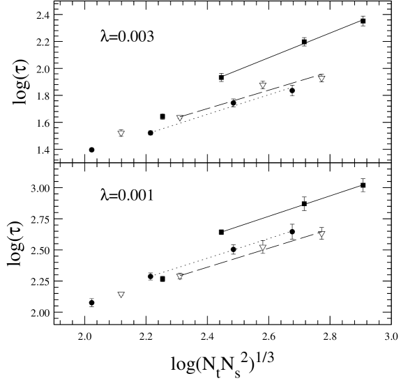
Figure 1: Logarithms of the autocorrelation times $\tau$ as a function of $\log(N_{t}N_{s}^{2})^{1/3}$, for $N_{t}=3$ (full circles), $N_{t}=4$ (empty triangles) and $N_{t}=6$ (full squares) and $N_{s}=12,16,24,32$. The straight lines are the fits for the dynamical exponents $z$ according to eq.(19). The points not covered by the fits correspond to $N_{s}=12$ and have not been used for the computation of the fits.

We have measured the integrated autocorrelation times $\tau$. The values obtained from the $\kappa$-energy, $\lambda$-energy and magnetisation are totally compatible. They oscillate, in units of $10\times(3~{}Metropolis+20~{}Clusters)$, approximately from $\tau\simeq 3$ in the best case (largest $\lambda$ and smallest lattice) to $\tau\simeq 38$ in the worst (smallest $\lambda$ and largest lattice). In particular we have estimated the dynamical exponent $z$ defined by

$$\tau\sim{(N_{t}\times{N_{s}}^{2})}^{z/3}$$ (19)

with fixed $N_{t}$, obtaining $z=0.8(1)$. This estimate is not totally rigorous because the autocorrelation times have been measured at the simulation points which do not coincide exactly with the ’critical’ ones (but they do it approximately). However it should be basically correct because, as can be seen in Figure 1, a power law with a rather well defined exponent is observed for the largest lattices. Figure 1 shows how $\tau$ scales with $N_{s}$, for fixed $N_{t}=3,4,6$ at $\lambda=0.001$ and $\lambda=0.003$. The fits have been computed using only the data relative to $N_{s}=16,24,32$, but for completeness in the figure we have displayed also the points corresponding to $N_{s}=12$. They give an exponent $z$ oscillating between $0.7$ and $0.9$ approximately. Metropolis alone would give a value $z=2$ while the Wolff algorithm, in spin systems where can it be used by itself, has $z=0$ because at the critical point the clusters can have any size. In our case the clustering is only able to change the sign of the fields, but its non-locality contributes to diminish significantly the dynamical Metropolis exponent.

For the sake of completeness, we have also determined the approximate position of the critical line at zero temperature. In this case no extrapolation to the thermodynamical limit has been made, and we have simulated only a $16^{3}$ lattice.

In order to estimate the critical points, we have used the Binder cumulant defined as:

$$U_{N_{s}}(\kappa)=\frac{3}{2}-\frac{\langle M^{4}\rangle}{2\langle M^{2}\rangle^{2}}$$ (20)

where

$$M=|(1/V)\sum_{\mbox{\scriptsize\boldmath$r$}}\phi_{\mbox{\scriptsize\boldmath$r$}}|$$ (21)

is the magnetisation or expectation value of the field, $V=N_{t}\times N_{s}^{2}$ being the volume.

At several points on the CCP’s, we have measured the second moment correlation length on the symmetric lattice $16^{3}$, in order to check the scaling. It is defined as [8, 26]

$$\xi=\left(\frac{1}{2d}\frac{\sum_{\mbox{\scriptsize\boldmath$x$}}{|x|}^{2}G(x)}{\sum_{\mbox{\scriptsize\boldmath$x$}}G(x)}\right)^{1/2},$$ (22)

where $G(x)$ is the correlation function. Usually this quantity is measured in the disordered phase, while we need evaluate it in the broken phase. There $\langle M\rangle\neq 0$ and then we have to use the connected correlation function

$$G(x,y)=G(x-y)=\langle\phi_{x}\phi_{y}\rangle-\langle\phi_{x}\rangle\langle\phi_{y}\rangle.$$ (23)

Using the lattice symmetries, $\xi$ can be expressed as

$$\xi=\left(\frac{\frac{\chi}{F}-1}{4sin^{2}\frac{\pi}{N}}\right)^{1/2}$$ (24)

where $N=N_{s}=N_{t}$ is the lattice size, $\chi$ is the susceptibility

$$\chi=\sum_{\mbox{\scriptsize\boldmath$x$}}G(x)=V(\langle M^{2}\rangle-{\langle M\rangle}^{2})$$ (25)

and $F$ is the analogous quantity at the smallest nonzero momentum (having two null components and one equal to $\pm 2\pi/N$)

$$F=\sum_{\mbox{\scriptsize\boldmath$x$}}G(x)e^{ip\cdot x}=\frac{1}{3V}\langle{|\sum_{\mbox{\scriptsize\boldmath$r$}}\phi_{\mbox{\scriptsize\boldmath$r$}}e^{2\pi ir_{1}/L}|}^{2}+{|\sum_{\mbox{\scriptsize\boldmath$r$}}\phi_{\mbox{\scriptsize\boldmath$r$}}e^{2\pi ir_{2}/L}|}^{2}+{|\sum_{\mbox{\scriptsize\boldmath$r$}}\phi_{\mbox{\scriptsize\boldmath$r$}}e^{2\pi ir_{3}/L}|}^{2}\rangle$$ (26)

$r_{j}$ being the components of $r$ (indeed, the fact of being in the ordered phase is irrelevant as far as $F$ is concerned, because the disconnected part cancels out from the sum due to the Fourier factor).

6 Results

6.1 Phase diagram

As explained in the previous section, for each pair ($N_{t},\lambda$) we have used $N_{s}=12,16,24,32$. As the field is not compact, it is difficult to obtain the critical points from observables like the specific heat and the susceptibility. An estimate of the critical point for each value of $N_{s}$ could be obtained from the maximum of the derivative of the cumulant $U_{N_{s}}(\kappa)$. However, in order to minimize finite size effects, we have rather used the intersections $\kappa^{*}(N_{s_{1}},N_{s_{2}})$ among all possible pairs of curves $U_{N_{s}}(\kappa)$, because the differences between them come only from the corrections to scaling. After simulating one value of $\kappa$ for every $N_{s}$ (having fixed $N_{t}$ and $\lambda$), we have computed $U_{N_{s}}(\kappa)$ in a narrow interval around the simulation point by means of the SDM. The simulation point was known to be near the critical line thanks to some hysteresis or from the estimations for the lattices simulated previously. Figure 2 shows $U_{N_{s}}(\kappa)$ for the different values of $N_{s}$, with $N_{t}=2$ and $\lambda=0.003$, as an example. The full marks correspond to the simulation points, while the empty ones are the extrapolated values.

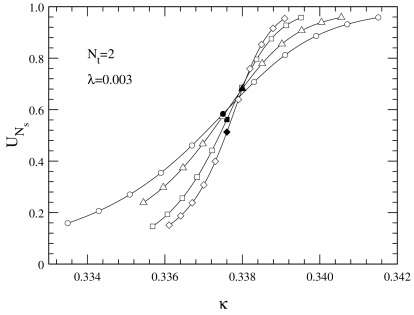
Figure 2: The Binder cumulants $U_{N_{s}}$ as a function of the hopping parameter $\kappa$, for the lattices with $N_{s}=12$ (circles), $N_{s}=16$ (triangles), $N_{s}=24$ (squares), $N_{s}=32$ (diamonds). The full marks are the simulation points, while the empty ones are extrapolations via the SDM.

Starting from the intersections $\kappa^{*}(N_{s_{1}},N_{s_{2}})$, the critical value $\kappa_{c}$ in the thermodynamic limit $N_{s}\to\infty$ can be estimated by using the following law [25]

$$\kappa^{*}(N_{s},bN_{s})-\kappa_{c}=\frac{1-b^{-\omega}}{b^{1/\nu}-1}{N_{s}}^{-\omega-1/\nu}$$ (27)

where $\omega$ is the exponent for the corrections-to-scaling. Since the scaling parameter is $N_{s}$, while $N_{t}$ is fixed, according to the hypothesis of dimensional reduction and universality, we have used the exponents of the Ising model in two dimensions, namely $\nu=1$, $\omega\simeq 4/3$ [13], obtaining satisfactory fits. To give an idea of their quality, in Figure 3 we show two extreme cases, smallest $\lambda$ - largest $N_{t}$ and largest $\lambda$ - smallest $N_{t}$, which are among the worst and the best fits respectively.

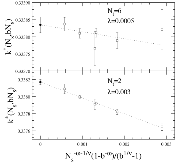
Figure 3: Intersections of Binder cumulants $\kappa^{*}(N_{s},bN_{s})$ as a function of $\frac{1-b^{-\omega}}{b^{1/\nu}-1}N_{s}^{-\omega-1/\nu}$ (squares). The dotted lines are the fits according to eq. (27). The full circles are the extrapolated values for $\kappa_{c}$ in the limit $N_{s}\rightarrow\infty$.

On the other hand, as a further justification for the use of the two-dimensional exponents, we have studied the scaling of the maximum derivative of the Binder cumulant with $N_{s}$. It was expected to scale like ${N_{s}}^{1/\nu}$ and we have checked this behavior for every pair ($N_{t},\lambda$), obtaining a good scaling and values of $\nu$ close to $1$ in every case ($\nu$ ranges from $0.95$ to $0.99$, and is in all cases almost compatible with $1$ within the errors). Figure 4 shows such a fit for $N_{t}=3$, $\lambda=0.001$.

Figure 4: Logarithms of the maximal Binder cumulant derivatives as a function of $N_{s}$ for $N_{t}=3$, $\lambda=0.001$. The line is the fit to compute $\nu$.

Although we have not made an exhaustive study of the order of the transitions, all the indications point towards the expected second order. One element is the value of the exponent $\nu$ obtained. Another is that no clear discontinuity is observed in the histograms for the lattices that we have simulated. In Figure 5 we plot the histograms of the $\kappa$-energy for $N_{t}=6$, $N_{s}=16,24,32$ at the point $\lambda=0.003$, $\kappa=0.3364$, which is very close to the transition line.

$\lambda$	$\kappa_{c}(N_{t}=6)$	$\kappa_{c}(N_{t}=4)$	$\kappa_{c}(N_{t}=3)$	$\kappa_{c}(N_{t}=2)$
0.003	0.336211(30)	0.336648(17)	0.337024(30)	0.338170(29)
0.002	0.335249(19)	0.335567(27)	0.336007(27)	0.336711(24)
0.001	0.334373(9)	0.334597(21)	0.334751(26)	0.335243(45)
0.0005	0.333835(23)	0.333924(19)	0.334024(35)	0.334237(16)

Table 1: Critical values $\kappa_{c}$ for the different values of $N_{t}$ and $\lambda$.

Figure 5: Hystogram of the configurations distribution as a function of the term in the action eq.(7) proportional to the hopping parameter $\kappa$, for $N_{t}=6$, $\lambda=0.003$ and $\kappa=0.3364$, $N_{s}=16$ (dots), $24$ (dashes), $32$ (solid).

In table 1 we quote the values of $\kappa_{c}$ for the different ($N_{t},\lambda$) studied. In order to have a continuous transition line for every value of $N_{t}$, we have made a linear extrapolation between each pair of correlative $\lambda$ values. Adding the critical line computed for the symmetric lattice (estimated on a $16^{3}$ lattice at $\lambda=0.001,0.003$ and then continued up to the gaussian point) we have obtained the phase diagram shown in Figure 6, where we have also included the CCP’s we have used for the determination of $T^{c}$.

Figure 6: Critical lines (solid curves) for $N_{t}=2,3,4,6$. The dashed line is the ’critical’ line for the symmetric lattice $16^{3}$. The dotted lines are the CCP’s $A,B,C,D$.

6.2 Critical temperatures

Now we have to search for the intersections of some CCP’s with the transition lines for the different values of $N_{t}$. The region of the phase diagram that we have computed limits the window of accessible CCP’s, as we could only use CCP’s whose intersections with the critical lines are in the range $0.0005<\lambda<0.003$. In addition, in order to ensure that we were exploring a region of continuum physics, we have required a good scaling of the correlation length along the trajectories. Trajectories below $D$ in Figure 6 intersect only the critical lines with $N_{t}=2,3$ and then have been discarded. Trajectories above $A$ have shown a poor scaling and have also been eliminated. This could depend on two circumstances: on one side the scaling region might be too near the gaussian point for these trajectories, on the other it is quite possible that near the critical line the finite size effects in the measurement of the correlation length are important.

These considerations have led us to consider only the trajectories included in the region of the phase diagram bounded by the curves $A$ and $D$ in Figure 6. All in all, we have used four trajectories, $A$, $B$, $C$ and $D$, starting from the points with $\lambda=0.003$ and $\kappa=0.3382$, $0.3389$, $0.3395$, $0.3402$ respectively. Among them, the only one cutting the critical line for $N_{t}=6$ is $A$, but it does it almost tangentially and the error in the determination of the intersection point is consequently very large. This produces an error still larger in the estimate of the temperature because in the proximity of the gaussian point the lattice spacing $a$ changes very rapidly along the CCP. As a matter of fact we have not been able to use $N_{t}=6$ for the measurement of the critical temperature and we had to limit ourselves to the crossings of the CCP’s with the critical lines for $N_{t}=2,3,4$.

$N_{t}$	$\kappa$	$\lambda$	$\xi$	$\xi\cdot s$	$\frac{-16{\pi}^{2}m^{2}(T_{N_{t}})}{g^{2}}$	$\frac{4\pi T_{N_{t}}}{g}$
2	0.33810(8)	0.00296(3)	3.42(3)	3.38(3)	17.275(2)	10.11(11)
3	0.33584(9)	0.00187(5)	5.78(9)	3.65(6)	17.268(4)	10.55(28)
4	0.33489(7)	0.00130(4)	8.84(12)	3.91(6)	17.256(5)	11.29(35)
2	0.33722(6)	0.00236(3)	3.75(5)	2.98(4)	22.389(2)	12.64(14)
3	0.33536(8)	0.00148(5)	7.10(14)	3.59(7)	22.381(5)	13.23(38)
4	0.33469(6)	0.00110(3)	9.36(16)	3.53(6)	22.381(5)	13.29(39)
2	0.33674(6)	0.00202(3)	3.94(8)	2.70(6)	26.829(2)	14.68(17)
3	0.33508(8)	0.00127(4)	7.27(32)	3.15(15)	26.821(5)	15.45(48)
4	0.33456(9)	0.00097(5)	9.92(28)	3.31(10)	26.825(9)	15.06(86)
2	0.33634(7)	0.00175(3)	4.11(8)	2.45(5)	32.074(3)	16.95(26)
3	0.33486(7)	0.00109(4)	8.02(25)	3.02(10)	32.065(6)	17.91(60)
4	0.33427(12)	0.00076(7)	10.93(19)	2.86(6)	32.052(16)	19.28(1.89)

Table 2: Correlation lengths $\xi$ and estimates $T_{N_{t}}$ of the critical temperatures associated with the crossings of the CCP’s $A,B,C,D$ (from top to bottom) with the critical lines of the lattices with $N_{t}=2,3,4$.

In table 2 we show the values of $\kappa$ and $\lambda$ at the points where the trajectories $A$, $B$, $C$ and $D$ (from up to down) intersect the critical lines for $N_{t}=2,3,4$. Their errors come from the deviations in the estimation of the critical lines, and have been calculated as explained below for the critical temperatures.

In correspondence with these intersection points we have measured the correlation length on a $16^{3}$ lattice in order to verify its scaling. We have chosen these and not any other points on the CCP’s because the good or poor scaling of $\xi$ just there indicates which values of $N_{t}$ we will be able to use for estimating the critical temperature in the continuum. The values of $\xi$ obtained are quoted in table 2. The errors quoted are the ones arising from the simulation and have been calculated with the jackknife method.

When going towards the gaussian point, $\xi$ should grow inversely to the parameter $s$, i.e. inversely to $a$ (see. eq.(12)) and thus the product $\xi\cdot s$ should be constant along the trajectory (the absolute scale of $s$ is of course arbitrary and, for each CCP, we have taken $s=1$ at its starting point). It is apparent from table 2 that for the trajectories $B$, $C$ and $D$ the values of $\xi\cdot s$ for $N_{t}=3,4$ are fully compatible within the errors, while for $N_{t}=2$ there are significant deviations from scaling. For the trajectory $A$ the result is less satisfactory, something that will be reflected also in a small difference among the estimates for the critical temperature resulting from $N_{t}=3$ and $4$ for this trajectory.

As we said above, we have constructed the critical lines by means of a linear interpolation of the critical points obtained numerically and have then used them to estimate the intersections with the CCP’s. From Figure 6 it is apparent that this is a rather good approximation. We have estimated the errors in the measurement of $T_{N_{t}}/g$ and ${m^{2}_{MS}}/g^{2}$ in the following way. In addition to the line formed by joining the values of $\kappa_{c}(\lambda)$ for the four values of $\lambda$ simulated, we have considered two more lines, on the two sides of the previous one. One has been obtained by joining the points corresponding to the upper values $\kappa_{c}(\lambda)+\sigma(\kappa_{c}(\lambda))$ and the other by joining the points corresponding to the lower values $\kappa_{c}(\lambda)-\sigma(\kappa_{c}(\lambda))$, $\sigma(\kappa_{c}(\lambda))$ being the error in the determination of $\kappa_{c}(\lambda)$. Each of the three lines gives a different estimate for the observables. We have taken as our estimate the one given by the central line and the error has been taken to be one half of the difference between the values given by the two external lines. This procedure would overestimate the error if the critical lines between the critical points computed were really straight; this overestimation should approximately compensate for the error introduced by the linearization.

The values of $T_{N_{t}}/g$ and ${m^{2}_{MS}}/g^{2}$ obtained in this way are shown in table 2 (multiplied by the constant factors $4\pi$ and $-16\pi^{2}$ in order to compare directly with the results in [15]). It can be seen how, for $N_{t}=3,4$, $T_{N_{t}}/g$ has reached a well defined limit (only for the trajectory $A$ the values of $T_{3}/g$ and $T_{4}/g$ are not perfectly compatible within the errors).

In order to check eq.(13), we have performed a series of best fits. To this purpose we have used all the data relative to $N_{t}=3,4$, except the point corresponding to the intercept of trajectory $A$ with the critical line for $N_{t}=3$, for the reason explained above. Some care has been necessary, because not all the data are statistically independent. Consider for instance the intercepts of trajectories $B,C,D$ with the critical line for $N_{t}=3$: they belong to the same straight segment of the interpolated critical line, which implies that among them only two are statistically independent of each other, while the third can be determined thereof. For this reason, we could not use all the data at once in a single fit; rather we have repeated the fits for all possible maximal subsets of statistically independent points extracted from the data. It turned out that all subsets consisted of five points out of a total of seven. The plots of $\chi^{2}(k)$ for all the combinations of data are displayed in Figure 7 (notice that $\chi^{2}(k)$ is not normalised per degree of freedom).

Figure 7: Plots of $\chi^{2}$ as a function of the parameter $k$ in eq.(13) for all maximal subsets of statistically independent data extracted from table 2 (the point relative to the CCP $A$ and $N_{t}=3$ has been excluded, so as all those of $N_{t}=2$). The number of degrees of freedom in all cases is $5-1=4$.

As can be seen from the figure, the errors on the estimates of $k$ (equal to semi-widths of the intervals in $k$, around the minimum, for which the variation of $\chi^{2}$ is less than $1$) are comparable for all the combinations of data and are around $0.15$. It is apparent that in all cases the minimum value of $\chi^{2}(k)$ per degree of freedom (four) is very good, which indicates that the fits can be trusted. The values of $k$ obtained from the fits are all practically consistent with each other, within the errors. As our final estimate, we have taken their average, while for the error we have taken a value larger than the individual errors, in such a way that all the fits are compatible with it. In conclusion, we have got: $k=2.1(2)$. The final fit is shown in Figure 8,where the curve having $k=1$ is also displayed for comparison.

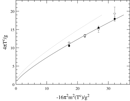
Figure 8: Estimates $T_{N_{t}}$ of the critical temperature as a function of the renormalised parameters $m^{2}_{MS}(T_{N_{t}})$ and $g$, for the CCP’s $A,B,C,D$ (from left to right), $N_{t}=3$ (full circles) and $N_{t}=4$ (empty triangles). The solid line is the fit according to eq.(13), with $k=2.1$. The dotted line corresponds to $k=1$.

7 Conclusions

We have investigated the phenomenon of symmetry restoration at finite temperature in the scalar $\lambda\phi^{4}_{3}$ model, by means of a Monte Carlo simulation. Using FSS techniques we have carefully determined the critical lines separating the ordered and the unordered phases on asymmetric lattices, for a number of different extensions in the temporal direction. The intersections of these lines with various RG trajectories lying in the ordered phase of the $T=0$ theory provide estimates of the critical temperature. The analysis of the results for lattices with increasing extensions in the time-direction clearly shows that these temperatures approach a well-defined finite value in the continuum limit, confirming the expectation of a symmetry restoring phase transition at a finite physical temperature for the continuum theory. We have measured $T^{c}$ for various RG trajectories. In this way we have checked the validity of the following equation relating $T^{c}$ to the renormalized parameters of the continuum theory:

$$T^{c}\log\left(\frac{4\pi kT^{c}}{g}\right)=-\frac{8\pi m^{2}_{MS}(T^{c})}{g}~{},$$

which was derived in [15] using renormalization group methods, and have been able to measure the so far unknown parameter $k$, obtaining the value $k=2.1(2)$.

8 Acknowledgments

The authors are grateful to J.L. Alonso, M. Asorey, J.M. Carmona and L.A. Fernández for discussions while the manuscript was in preparation. This work is partially supported by CICyT AEN94-0218, and AEN95-1284-E. D. Iñiguez and C.L. Ullod are MEC and DGA fellows respectivelly.

References

- [1] D.A.Kirzhnits and A.D.Linde, Phys. Lett. B 42 (1972) 471.
- [2] S. Weinberg, Phys. Rev. D 9 (1974) 3357.
- [3] L. Dolan and R. Jackiw, Phys. Rev. D 9 (1974) 3320.
-
[4]
R.N. Mohapatra and G. Senjanović, Phys. Lett.
B 89 (1979) 57; Phys. Rev. Lett. 42 (1979) 1651; Phys. Rev. D 20
(1979) 3390;
P. Salomonson, B.-S. Skagerstam and A. Stern, Phys. Lett. B 151 (1985) 243;
G. Dvali, A. Melfo and G. Senjanović, Phys. Rev. Lett. 75 (1995) 4559. -
[5]
Y. Fujimoto and S. Sakakibara, Phys. Lett. B 151 (1985) 260;
G.A. Hajj and P.N. Stevenson, Phys. Rev: D 37 (1988) 413;
G. Bimonte and G. Lozano, Phys. Lett. B 366 (1996) 248; Nucl. Phys. B 460 (1996) 155 and references therein;
G. Amelino-Camelia, Nucl. Phys. B 476 (1996) 255. -
[6]
S. Bornholdt, N. Tetradis and C. Wetterich, Phys. Rev.
D 53 (1996) 4552;
N. Tetradis and C. Wetterich, Int. Jour. Mod. Phys. A 9 (1994) 4029 and references therein. -
[7]
K. Kajantie, M. Laine, K. Rummukainen and
M. Shaposhnikov, Phys. Rev. Lett. 77 (1996) 2887;
K. Farakos, K. Kajantie, K. Rummukainen and M. Shaposhnikov, Nucl. Phys. B 442 (1995), 317; B 425 (1994), 67; and references therein;
F. Csikor et al, Nucl. Phys. B (Proc. Suppl.) 42 (1995) 569;
The RTN Collaboration, J.L. Alonso et al, Nucl. Phys. B 405 (1993) 574. - [8] F. Cooper, B. Freedman and D. Preston, Nucl. Phys. B 210 (1982) 210.
- [9] B. Freedman, P. Smolensky and D. Weingarten, Phys. Lett. B 113 (1982) 481.
- [10] C. Domb and J.C. Lebowitz, Phase Transitions and critical phenomena, Vol 9. (Academic Press, New York, 1984).
- [11] F. Cooper and B. Freedman, Nucl. Phys. B 239 (1984) 459.
- [12] R.A. Weston, Phys. Lett. B 219 (1989) 315.
- [13] J. Zinn-Justin, Quantum Field Theory and critical phenomena, (Clarendon Press, Oxford, 1990).
- [14] Y. Fujimoto, A. Wipf and H. Yoneyama, Zeit. Phys. C 35 (1987) 351.
- [15] M.B. Einhorn and D.R.T. Jones, Nucl. Phys. B 398 (1993) 611.
- [16] C. King and L.G. Yaffe, Comm. Math. Phys. 108 (1987) 423.
- [17] G. Bimonte and G. Lozano, preprint DFTUZ/96/11 and Imperial/TP/95-96/34, hep-th/9603201, in press on Phys. Lett. B.
-
[18]
Y. Fujimoto, A. Wipf and H. Yoneyama,
Phys. Rev. D 38 (1988) 2625;
- [19] H. Li and T-l Chen, Phys. Lett. B 347 (1995) 131.
- [20] M.G. do Amaral, C. Aragão de Carvalho, M.E. Pol and R.C. Shellard, Zeit. Phys. 32 C (1986) 609.
- [21] J.I. Kapusta, Finite-temperature field theory, (Cambridge University Press, Cambridge, 1989).
- [22] J.C. Ciria and A. Tarancón, Phys. Rev. D 49 (1994) 1020.
- [23] U. Wolff, Phys. Rev. Lett. 62 (1989) 3834.
-
[24]
M. Falcioni et al, Phys. Lett. B 108 (1982) 331;
A.M. Ferrenberg and R. Swendsen, Phys. Rev. Lett. 61 (1988) 2635. - [25] K. Binder, Z. Phys. 43 (1981) 119.
-
[26]
J.K. Kim, Phys. Rev. Lett. 70 (1993) 1735;
S. Caracciolo, R.G. Edwards, A. Pelissetto and A.D. Sokal, Nucl. Phys. B 403 (1993) 475.