UTHEP-349 1996 Chiral zero modes on the domain-wall model
in 4+1 dimensions

Abstract

We investigate an original domain-wall model in 4+1 dimensions numerically in the presence of U(1) dynamical gauge field only in an extra dimension, corresponding to a weak coupling limit of 4-dimensional physical gauge coupling. Using a quenched approximation we carry out numerical simulation for this model at $\beta_{s}(=1/g^{2}_{s})=$ 0.29 (“symmetric” phase) and 0.5 (“broken” phase), where $g_{s}$ is the gauge coupling constant of the extra dimension. In the broken phase, we found that there exists a critical value of a domain-wall mass $m_{0}^{c}$ which separates a region with a fermionic zero mode on the domain wall from the one without it in the same case of (2+1)-dimensional model. On the other hand, in the symmetric phase, our numerical data suggest that the chiral zero modes disappear in the infinite limit of 4-dimensional volume. From these results it seems difficult to construct the U(1) lattice chiral gauge theory via an original domain-wall formulation.

I Introduction

Although perturbative aspects of electro-weak interaction are well described by the standard model, its non-perturbative phenomenon such as baryon number asymmetry have to be investigated beyond the perturbation theory. At present, the most powerful non-perturbative technique is the lattice field theory. However it is non-trivial to define the standard model on a lattice since it is a type of chiral gauge theories, construction of which is one of the long-standing problem of lattice field theory: Because of the fermion doubling problems, a naively $D$-dimensional discretized lattice fermion field yields $2^{D}$ fermion particles, half of one chirality and half of the other, so that the theory becomes non-chiral[1]. Several lattice approaches have been proposed, but so far none of them have been proven to work successfully[2].

D. Kaplan has proposed a new construction of lattice chiral gauge theories via domain-wall models[3]. Starting from a vector-like gauge theory in $2k+1$ dimensions with a fermion mass term being a shape of a domain-wall in the (extra) $(2k+1)$th dimension, he showed in the weak gauge coupling limit that a massless chiral state arises as a zero mode bound to the $2k$-dimensional domain-wall while all the doublers have large masses of the lattice cut-off scale. It has been also shown that the model works well for smooth background gauge fields[4, 5, 6, 7].

Two simplified variants of the original Kaplan’s domain-wall model have been proposed: an “overlap formula”[8, 9] and a “waveguide model”[10, 11]. Gauge fields appeared in these variants are $2k$-dimensional and are independent of the extra $(2k+1)$th coordinate, while those in the original model are $(2k+1)$-dimensional and depend on the extra $(2k+1)$th coordinate. These variants work successfully for smooth background gauge fields [12, 13, 14, 15, 16, 17, 18, 21], as the original one does. Non-perturbative investigations for these variants seems easier than that for the original model due to the simpler structure of gauge fields.

However it has been reported[10, 11] that the waveguide model in the weak gauge coupling limit cannot produce chiral zero modes needed to construct chiral gauge theories. In this limit, if gauge invariance were maintained, pure gauge field configurations equivalent to the unity by gauge transformation would dominate and gauge fields would become smooth. In the set-up of the waveguide model, however, $2k$-dimensional gauge fields are non-zero only in the layers near domain wall (waveguide) , so that the gauge invariance is broken in the edge of the waveguide. Therefore, even in the weak gauge coupling limit, gauge fields are no more smooth and become very “rough”, due to the gauge degrees of freedom appeared to be dynamical in this edge. As a result of the rough gauge dynamics, a new chiral zero mode with the opposite chirality to the original zero mode on the domain wall appears in the edge, so that the fermionic spectrum inside the waveguide becomes vector-like. It has been claimed[10, 11] that this “rough gauge problem” also exists in the overlap formula since the gauge invariance is broken by the boundary condition at the infinity of the extra dimension[17, 18]. Furthermore an equivalence between the waveguide model and the overlap formula has been pointed out for the special case[19]. Although the claimed equivalence has been challenged in Refs.[20, 21], it is still crucial for the success of the overlap formula to solve the “rough gauge problem” and to show the existence of a chiral zero mode in the weak gauge coupling limit.

In the original model there are two inverse gauge couplings $\beta=1/g^{2}$ and $\beta_{s}=1/g_{s}^{2}$, where $g$ is the coupling constant in (physical) $2k$ dimensions and $g_{s}$ is the one in the (extra) $(2k+1)$th dimension. Very little are known about this model except $\beta_{s}=0$ case[10, 22, 23] where the spectrum seems vector-like and the case of (2+1)-dimensional U(1) model[24]. Since perturbation theory for the physical gauge coupling $g$ is expected to hold, the fermion spectrum of the model can be determined in the limit that $g\rightarrow 0$. In this weak coupling limit, all gauge fields in the physical dimensions can be gauged away, while the gauge field in the extra dimension is still dynamical and its dynamics is controlled by $\beta_{s}$. Instead of the gauge degrees of freedom in the edge of the waveguide, $(2k+1)$th component of gauge fields represent roughness of $2k$-dimensional gauge fields. An important question is whether the chiral zero mode on the domain wall survives in the presence of this rough dynamics. The dynamics of the gauge field in this limit is equivalent to $2k$-dimensional scalar model with $2L_{s}$ independent copies where $2L_{s}$ is the number of sites in the extra dimension. In general at large $\beta_{s}$ such a system is in a “broken” phase where some global symmetry is spontaneously broken, while at small $\beta_{s}$ the system is in a “symmetric” phase. Therefore there exists a critical point $\beta_{s}^{c}$, and it is likely that the phase transition at $\beta_{s}=\beta_{s}^{c}$ is continuous (second or higher order). The “gauge field” becomes rougher and rougher at smaller $\beta_{s}$. Indeed we know that the zero mode disappears at $\beta_{s}=0$[22], while the zero mode exists at $\beta_{s}=\infty$ ( free case ). So far we do not know the fate of the chiral zero mode in the intermediate range of the coupling $\beta_{s}$. There are the following three possibilities: (a) The chiral zero mode always exists except $\beta_{s}=0$. In this case we may likely construct a lattice chiral gauge theory in both broken ($\beta_{s}>\beta_{s}^{c}$) and symmetric ($\beta_{s}<\beta_{s}^{c}$), and the continuum limits may be taken at $\beta_{s}=\beta_{s}^{c}$. This is the best case for the domain-wall model. (b) The chiral zero mode exists only in the broken phase ($\beta_{s}>\beta_{s}^{c}$). In this case the domain-wall method can describe a lattice chiral gauge theory in the broken phase at finite cut-off. However it is likely that the continuum limit taken at $\beta_{s}=\beta_{s}^{c}$ from above leads to a vector gauge theory. (c) No chiral zero mode survives except $\beta_{s}=\infty$. The original model can not describe lattice chiral gauge theories at all. It is very important to determine which possibility is indeed realized in the domain-wall model.

Instead of (4+1)-dimensional models, we have recently investigated a (2+1)-dimensional U(1) model[24]. Using a quenched approximation we have carried out a numerical simulation to see whether chiral zero modes exist or not in this model. In the weak coupling limit of the physical gauge coupling the (2+1)-dimensional U(1) gauge system is reduced to the 2-dimensional U(1) spin system . Strictly speaking, there is no order parameter in the 2-dimensional U(1) spin system. On a large but finite lattice, however, the behavior of the model is similar to the one of a 4-dimensional scalar model: On a finite lattice we regard the Kosterlitz-Thouless phase as the ”symmetric” phase and the spin-wave phase as the ”broken” phase. In the ”broken” phase we have numerically found that there exists a critical value of a domain-wall mass $m_{0}^{c}$ which separates a region with a fermionic zero mode on the domain wall from one without it. In the ”symmetric” phase the critical values of the domain wall mass seems to also exist but is very close to its upper bound $m_{0}=1$, so that the region with a fermionic zero mode is very narrow. Because of the difficulty observed in the numerical simulation near $m_{0}=1$ we cannot exclude a possibility that the existence of the zero mode is an artifact of finite lattice size effects. Further simulation we have made on larger lattice sizes can not give a definite conclusion. Since, as mentioned before, the phases of the model in the infinite volume limit is different from the ones of the 4-dimensional model, we did not attempt to increase lattice sizes further, for example $100^{2}$, to see the fate of zero mode in the symmetric phase. Instead we have decided to investigate the (4+1)-dimensional U(1) model directly, to obtain the definite conclusion on the existence of zero modes in the symmetric phase.

In this paper, in order to know the fate of the chiral zero mode, we have carried out a numerical simulation of a domain-wall model in 4+1 dimensions with a quenched U(1) gauge field in the $\beta=\infty$ limit. In Sec.2 , we have defined our domain-wall model with dynamical gauge fields. We have calculated a fermion propagator by using a kind of mean-field approximation, to show that there is a critical value of the domain-wall mass parameter above which the zero mode exist. The value of the critical mass may depend on $\beta_{s}$, which controls the dynamics of the gauge field. In Sec.3 , we have calculated the fermion spectrum numerically using quenched approximation at $\beta_{s}=0.29,0.5$ and at various values of domain-wall masses. We have found that in the broken phase ($\beta_{s}=0.5$) there exists the range of a domain-wall mass parameter in which the chiral zero mode survives on the domain-wall. In the symmetric phase ($\beta_{s}=0.29$), however, from data on several lattice sizes we have found an numerical evidence that the chiral zero mode disappears in the infinite volume limit of 4-dimensional Euclidean space-time. Our conclusions and some discussions are given in Sec. 4.

II domain-wall model

A Definition of the model

We consider a vector gauge theory in $D=2k+1$ dimensions with a domain-wall mass term, which has a kink-like mass term in the coordinate of an extra dimension. This domain-wall model is originally proposed by Kaplan[3], and a fermionic part of the action is reformulated by Narayanan-Neuberger[8], in terms of a $2k$-dimensional theory. The model is defined by the action

$$S=S_{G}+S_{F},$$ (1)

where $S_{G}$ is the action of a dynamical gauge field , $S_{F}$ is the fermionic action. $S_{G}$ is given by

$$S_{G}=\beta\sum_{n,\mu>\nu}\sum_{s}\left\{1-{\rm ReTr}\left[U_{\mu\nu}(n,s)\right]\right\}+\beta_{s}\sum_{n,\mu}\sum_{s}\left\{1-{\rm ReTr}\left[U_{\mu D}(n,s)\right]\right\},$$ (2)

where $\mu,\nu$ run from $1$ to $2k$ , $n$ is a $2k$-dimensional lattice point , and $s$ is a coordinate of an extra dimension. $U_{\mu\nu}(n,s)$ is a $2k$-dimensional plaquette and $U_{\mu D}(n,s)$ is a plaquette containing two link variables in the extra direction. $\beta$ is the inverse gauge coupling for the plaquette $U_{\mu\nu}$ and $\beta_{s}$ is the one for the plaquette $U_{\mu D}$ . In general , $\beta\neq\beta_{s}$ . The fermion action $S_{F}$ on the Euclidean lattice, in terms of the $2k$-dimensional notation, is given by

$$S_{F} = \frac{1}{2}\sum_{n\mu}\sum_{s}\bar{\psi}_{s}(n)\gamma_{\mu}\left[U_{s,\mu}(n)\psi_{s}(n+\mu)-U_{s,\mu}^{{\dagger}}(n-\mu)\psi_{s}(n-\mu)\right]$$ (5)

$$\mbox{}+\sum_{n}\sum_{s,t}\bar{\psi}_{s}(n)\left[M_{0}P_{R}+M_{0}^{{\dagger}}P_{L}\right]\psi_{t}(n)$$

$$\mbox{}+\frac{1}{2}\sum_{n\mu}\sum_{s}\bar{\psi}_{s}(n)\left[U_{s,\mu}(n)\psi_{s}(n+\mu)+U_{s,\mu}^{{\dagger}}(n-\mu)\psi_{s}(n-\mu)-2\psi_{s}(n)\right],$$

where $s,t$ are an extra coordinates , $P_{R/L}=\frac{1}{2}(1\pm\gamma_{2k+1})$ ,

$$\left\{\begin{array}[]{l}(M_{0})_{s,t}=U_{s,D}(n)\delta_{s+1,t}-a(s)\delta_{s,t}\\ (M_{0}^{{\dagger}})_{s,t}=U_{s-1,D}^{{\dagger}}(n)\delta_{s-1,t}-a(s)\delta_{s,t}.\end{array}\right.$$ (6)

Here $U_{s,\mu}(n),U_{s,D}(n)$ ($D=2k+1$) are link variables connecting a site $(n,s)$ to $(n+\mu,s)$ or $(n,s+1)$, respectively. Because of a periodic boundary condition in the extra dimension , $s,t$ run from $-L_{s}$ to $L_{s}-1$ , and $a(s)$ is given by

$$a(s) = 1-m_{0}\,{\rm{sign}}\left[(s+\frac{1}{2})\,{\rm{sign}}(L_{s}-s-\frac{1}{2})\right]$$ (7)

$$= \left\{\begin{array}[]{ll}1-m_{0}&\mbox{}(-\frac{1}{2}<s<L_{s}-\frac{1}{2})\\ 1+m_{0}&\mbox{}(-L_{s}-\frac{1}{2}<s<-\frac{1}{2})\,,\end{array}\right.$$ (10)

where $m_{0}$ is the height of the domain-wall mass. It is easy to check that the above fermionic action is identical to the one in $2k+1$ dimensions, proposed by Kaplan[3, 8].

In weak coupling limit of both $\beta$ and $\beta_{s}$ , it has been shown that at $0<m_{0}<1$ a desired chiral zero mode appears on a domain wall ($s=0$ plane) without unwanted doublers. Because of the periodic boundary condition in the extra dimension, however, a zero mode of the opposite chirality to the one on the domain wall appears on the anti-domain-wall $(s=L_{s}-1)$. Overlap between two zero modes decreases exponentially at large $L_{s}$. A free fermion propagator is easily calculated and an effective action of a (2+1)- and (4+1)-dimensional model including the gauge anomaly and the Chern-Simons term can be obtained for smooth background gauge fields[4, 5].

The original Kaplan’s domain-wall models in the 4+1 dimension, however, have not been investigated yet non-perturbatively, except $\beta_{s}=0$[10, 22, 23] and (2+1)-dimensional case[24]. Main question is whether the chiral zero mode survives in the presence of rough gauge fields mentioned in the introduction. To answer this question we will analyze the fate of the chiral zero mode in the weak coupling limit for $\beta$. In this limit, the gauge field action $S_{G}$ is reduced to

$$S_{G}=\beta_{s}\sum_{s}\sum_{n,\mu}\left\{1-{\rm ReTr}\left[V(n,s)V^{{\dagger}}(n+\mu,s)\right]\right\},$$ (11)

where the link variable $U_{s,D}(n)$ in the extra direction is regarded as a site variable $V(n,s)(=U_{s,D}(n))$. This action is identical to the one of a $2k$-dimensional spin model and $s$ is regarded as an independent flavor. The action eq.(11) is invariant under

$$V(n,s)\longrightarrow g(s)V(n,s)g^{{\dagger}}(s+1)\quad,\qquad(g(s)\in G),$$ (12)

where $G$ is the gauge group of the original model. Therefore the total symmetry of the model is $G^{2L_{s}}$, where $2L_{s}$, the size of the extra dimension, is regarded as the number of independent flavors. We use this (reduced) model for our numerical investigation.

B Mean field approximation for fermion propagators

When the dynamical gauge fields are added even on the extra dimension only, it is difficult to calculate the fermion propagator analytically. Instead of calculating the fermion propagator exactly, we use a mean-field approximation to see an effect of the dynamical gauge field qualitatively. The mean-field approximation we adopt is that the link variables are replaced as

$$V(n,s)\,\,\,\left(=U_{s,D}(n)\right)\,\,\,\longrightarrow z,$$ (13)

where $z$ is a $(n,s)$-independent constant. From eq.(5) the fermion action in a $2k$-dimensional momentum space becomes

$$S_{F}\rightarrow\sum_{s,t,p}\bar{\psi}_{s}(-p)\left(\sum_{\mu}i\gamma_{\mu}\sin(p_{\mu})\delta_{s,t}+\left[M(z)P_{R}+M^{{\dagger}}(z)P_{L}\right]_{s,t}\right)\psi_{t}(p),$$ (14)

$$(M(z))_{s,t}=(M_{0}(z))_{s,t}+\frac{\nabla(p)}{2}\delta_{s,t}\,,\,(M^{{\dagger}}(z))_{s,t}=(M^{{\dagger}}_{0}(z))_{s,t}+\frac{\nabla(p)}{2}\delta_{s,t}\,,\,\nabla(p)\equiv\sum_{\mu=1}^{D-1}2(\cos p_{\mu}-1),$$ (15)

$$(M_{0}(z))_{s,t}=z\delta_{s+1,t}-a(s)\delta_{s,t}\quad,\qquad(M^{{\dagger}}_{0}(z))_{s,t}=z\delta_{s-1,t}-a(s)\delta_{s,t}\quad.$$ (16)

Following Refs.[4, 5, 8] ,especially Ref.[5], it is easy to obtain a mean field fermion propagator on a finite lattice with the periodic boundary condition:

$$G(p)_{s,t}=$$ (17)

$$\left[\left\{\left(-i\sum_{\mu}\gamma_{\mu}\bar{p}_{\mu}+M(z)\right)G_{L}(p)\right\}_{s,t}P_{L}\right.+\left.\left\{\left(-i\sum_{\mu}\gamma_{\mu}\bar{p}_{\mu}+M^{{\dagger}}(z)\right)G_{R}(p)\right\}_{s,t}P_{R}\right],$$ (18)

$$G_{L}(p)=\frac{\displaystyle 1}{\displaystyle{\bar{p}^{2}+M^{{\dagger}}(z)M(z)}}\quad,\quad G_{R}(p)=\frac{\displaystyle 1}{\displaystyle{\bar{p}^{2}+M(z)M^{{\dagger}}(z)}}\quad,$$ (19)

with $\bar{p}_{\mu}\equiv\sin(p_{\mu})$. For large $L_{s}$ where we neglect terms of $O(e^{-cL_{s}})$ with $c>0$, $G_{L}$ and $G_{R}$ are given by

$$\left[G_{L}(p)\right]_{s,t}=\left\{\begin{array}[]{ll}Be^{-\alpha_{+}|s-t|}+\left(A_{L}-B\right)e^{-\alpha_{+}(s+t)}+\left(A_{R}-B\right)e^{-\alpha_{+}(2L_{s}-s-t)},&(s,t\geq 0)\\ A_{L}e^{-\alpha_{+}s+\alpha_{-}t}+A_{R}e^{-\alpha_{+}(L_{s}-s)-\alpha_{-}(L_{s}+t)},&(s\geq 0,t\leq 0)\\ A_{L}e^{\alpha_{-}s-\alpha_{+}t}+A_{R}e^{-\alpha_{-}(L_{s}+s)-\alpha_{+}(L_{s}-t)},&(s\leq 0,t\geq 0)\\ Ce^{-\alpha_{-}|s-t|}+\left(A_{L}-C\right)e^{\alpha_{-}(s+t)}+\left(A_{R}-C\right)e^{-\alpha_{-}(2L_{s}+s+t)},&(s,t\leq 0)\end{array}\right.$$ (20)

$$\left[G_{R}(p)\right]_{s,t}=\left\{\begin{array}[]{ll}Be^{-\alpha_{+}|s-t|}+\left(A_{R}-B\right)e^{-\alpha_{+}(s+t+2)}+\left(A_{L}-B\right)e^{-\alpha_{+}(2L_{s}-s-t-2)},&(s,t\geq-1)\\ A_{R}e^{-\alpha_{+}(s+1)+\alpha_{-}(t+1)}+A_{L}e^{-\alpha_{+}(L_{s}-s-1)-\alpha_{-}(L_{s}+t+1)},&(s\geq-1,t\leq-1)\\ A_{R}e^{\alpha_{-}(s+1)-\alpha_{+}(t+1)}+A_{L}e^{-\alpha_{-}(L_{s}+s+1)-\alpha_{+}(L_{s}-t-1)},&(s\leq-1,t\geq-1)\\ Ce^{-\alpha_{-}|s-t|}+\left(A_{R}-C\right)e^{\alpha_{-}(s+t+2)}+\left(A_{L}-C\right)e^{-\alpha_{-}(2L_{s}+s+t+2)},&(s,t\leq-1)\end{array}\right.$$ (21)

where

$$a_{\pm}=z(1-\frac{\nabla(p)}{2}\mp m_{0})=zb_{\pm},$$ (22)

$$\alpha_{\pm}={\rm{arccosh}}\left[\frac{\bar{p}^{2}+z^{2}+b_{\pm}^{2}}{2zb_{\pm}}\right],$$ (23)

$$A_{L}=\frac{1}{a_{+}e^{\alpha_{+}}-a_{-}e^{-\alpha_{-}}},\,A_{R}=\frac{1}{a_{-}e^{\alpha_{-}}-a_{+}e^{-\alpha_{+}}},$$ (24)

$$B=\frac{1}{2a_{+}\sinh\alpha_{+}}\quad,\quad C=\frac{1}{2a_{-}\sinh\alpha_{-}}.$$ (25)

Like a free fermion theory, the terms of $A_{R},B$ and $C$ have no singularity for all $z$ as $p\rightarrow 0$. A behavior of $A_{L}$ is, however, different. As $p\rightarrow 0$ $A_{L}$ behaves as

$$A_{L}\rightarrow\left\{\begin{array}[]{lcl}\frac{\displaystyle 1}{\displaystyle[(1-m_{0})^{2}-z^{2}]+O(p^{2})}&,&(0<m_{0}<1-z)\\ \\ \frac{\displaystyle 4m_{0}^{2}-[(z^{2}-1)-m_{0}^{2}]^{2}}{\displaystyle 4m_{0}z^{2}p^{2}}&,&(1-z<m_{0}<1).\end{array}\right.$$ (26)

A critical value of the domain-wall mass that separates a region with a zero mode and a region without zero modes is $m_{0}^{c}=1-z$. Since $A_{L}$ term dominates for $1-z<m_{0}<1$ in the $G_{L}$ (eq.(20)) and $G_{R}$ (eq.(21)), a right-handed zero mode appears in the $s=0$ plane , and a left-handed zero mode in the $s=L_{s}-1$ plane. For $0<m_{0}<1-z$ the right- and left-handed fermions are massive in all $s$-planes. Since the terms of $A_{L}(A_{R})$ and $B(C)$ are almost same value in this region of $m_{0}$, a translational invariant term dominates in $G_{L}$ and $G_{R}$ in the positive (negative) $s$-layer , so that the spectrum becomes vector-like.

If $z\rightarrow 1$ , the model becomes a free theory. The propagator obtained in this section agrees with the one obtained in Ref.[4]. In the opposite limit that $z\rightarrow 0$ , since there is no hopping term to the neighboring layers, this model becomes the one analyzed in Ref.[22] in the case of the strong coupling limit $\beta_{s}=0$ , and in Ref.[23] , in the case that $z$ is identified to the vacuum expectation value of the link variables. This consideration suggests that the region where the zero modes exist become smaller and smaller as $z$ $(1-z<m_{0}<1)$ approaches zero.

What corresponds to $z$ ? Boundary conditions which $z$ satisfies are $z=1$ at $\beta_{s}=\infty$ and $z=0$ at $\beta_{s}=0$. As explained before the gauge field action of our model is identical to that of the U(1) spin system in 4-dimensions. So the most naive candidate[23] is

$$z=\langle V(n,s)\rangle,$$ (27)

which is not invariant under the symmetry (12). In our simulations on $L^{3}\times L_{4}\times 2L_{s}$ lattices, as an order parameter, we take a vacuum expectation value of link variable calculated with rotational technique:

$$v=\langle\,\,\frac{1}{2L_{s}}\sum_{s}\left|\frac{1}{L_{4}L^{3}}\sum_{n}V(n,s)\right|\,\,\rangle\quad.$$ (28)

Although $v$ defined in eq.(28) is always non-zero on finite lattices, it becomes zero in the symmetric phase but stays non-zero in the broken phase in the infinite volume limit. Fig. 1(a) shows that, even on finite lattices, $v$ behaves as if it was an order parameter: it is very small and decreases as the volume increases in the would-be symmetric phase. If the identification that $z=v$ is true, zero modes disappear in the symmetric phase, where $v=0$. The other choice, which is invariant under (12), is the vacuum expectation value of plaquette:

$$z^{2}=\langle{\rm TrRe}\{V(n,s)V^{\dagger}(n+\mu,s)\}\rangle.$$ (29)

In this identification the zero modes always exist in both phases, since $\langle{\rm TrRe}\{V(n,s)V^{\dagger}(n+\mu,s)\}\rangle$ is non-zero for all $\beta_{s}$ except $\beta_{s}=0$ and is insensitive to which phase we are in, as shown in Fig. 1(b).

III numerical study of (4+1)-dimensional U(1) model

A Method of numerical calculations

In this section we numerically study the domain-wall model in 4+1 dimensions with a U(1) dynamical gauge field in the extra dimension. As seen from eq.(11) , the gauge field action can be identified with a 4-dimensional U(1) spin model (with $2L_{s}$ copies).

Our numerical simulation has been carried out by the quenched approximation. Configurations of U(1) dynamical gauge field are generated and fermion propagators are calculated on these configurations. The obtained fermion propagators are gauge non-invariant in general under the symmetry (12). The fermion propagator $G(p)_{s,t}$ becomes “invariant” if and only if $s=t$. Thus, we take the $s-s$ layer as propagating plane ($\approx$ “physical space”), and investigate the behavior of the fermion propagator in this layer.

To study the fermion spectrum, we first extract $G_{L}$ and $G_{R}$, defined in eq.(18), from the fermion propagator. Assuming eq.(19), we then obtain corresponding “fermion masses” from $G_{L}^{-1}(p)$ and $G_{R}^{-1}(p)$ by fitting them linearly in $\bar{p}^{2}$ as follows.

$$G_{L}^{-1} = \bar{p}^{2}+M^{{\dagger}}M\rightarrow m_{f}^{2}({\rm{Right}})\quad,\quad(p\rightarrow 0),$$ (30)

$$G_{R}^{-1} = \bar{p}^{2}+MM^{{\dagger}}\rightarrow m_{f}^{2}({\rm{Left}})\quad,\quad(p\rightarrow 0).$$ (31)

We take the following setup for 4-dimensional momenta. A periodic boundary condition is taken for the 1st- 2nd- 3rd-direction and the momenta in these directions are fixed on $p_{1},p_{2},p_{3}=0$. An anti-periodic boundary condition is taken for the 4th-direction and the momentum in this direction is variable, $p_{4}=(2n+1)\pi/L_{4}\,,\,n=-L_{4}/2,...,L_{4}/2-1$, where $L_{4}$ is the number of site of 4th direction. (Our numerical simulations have been performed always for $L_{4}=32$.)

B Simulation parameters

From Fig. 1(a) it is inferred that the system is in the symmetric phase at $\beta_{s}=0.29$ and in the broken phase at $\beta_{s}=0.5$. Our simulation is performed in the quenched approximation on $L^{3}\times 32\times 2L_{s}$ lattices with $L=$4, 6, 8 and $L_{s}=8$ at $\beta_{s}=$ 0.29 (symmetric phase) , where $L$ is a lattice size of 1st- 2nd- 3rd-direction, and on $L^{3}\times 32\times 2L_{s}$ lattices with $L=$4, 6, 8 and $L_{s}=8$ at $\beta_{s}=$ 0.5 (broken phase). The coordinate $s$ in the extra dimension runs $-8\leq s\leq 7$. Gauge configurations are generated by the 5-hit Metropolis algorithm. For the thermalization first 5000 sweeps are discarded.

The fermion propagators are calculated by the conjugate gradient method on 50 configurations separated by 100 sweeps. We take the domain-wall mass $m_{0}=$ 0.7 , 0.8 , 0.9 , 0.95 , 0.99 at $\beta_{s}=$ 0.29 and $m_{0}=$ 0.1 , 0.2 , 0.3 , 0.4 , 0.5 , 0.6 , 0.9 at $\beta_{s}=$ 0.5. As mentioned before, the boundary conditions in 1st- 2nd- 3rd- and 5th-directions are periodic and the one in 4th-direction is anti-periodic. Wilson parameter $r$ has been set to $r=1$. The fermion propagators have been investigated mainly at $s=$ 0 , $-1$. These $s$ are the layers where we put sources. The layer at $s=0$ is the domain wall. Errors are all estimated by the jack-knife method with unit bin size.

C Fermion spectrum in the broken phase

The system is in broken phase at $\beta_{s}=$ 0.5. We first consider the fermion spectrum on the layer at $s=0$. Let us show Fig. 2, which is a plot of the $G_{L}^{-1}$ and $G_{R}^{-1}$ as a function of $\bar{p}_{4}^{2}\equiv\sin^{2}(p_{4})$ at $m_{0}$ =0.1 and 0.6. (Note we always set $p_{1},p_{2},p_{3}=0$.) In the limit $p_{4}\rightarrow 0$, $G_{R}^{-1}$ remains non-zero at both $m_{0}$, while $G_{L}^{-1}$ vanishes at $m_{0}=0.6$. We obtain the value of $m_{f}^{2}$, which can be regarded as the mass square in $4$-dimensional world, by the linear fit in $\bar{p}_{4}^{2}$ near $\bar{p}_{4}^{2}=0$, and plot $m_{f}$ as a function of $m_{0}$ in Fig. 3. The mass of right-handed fermion, obtained from $G_{L}^{-1}$, becomes very small (less than 0.1) at $m_{0}$ larger than $0.35$, so we conclude that the critical value is $m_{0}^{c}\sim 0.35$. Whenever the domain-wall mass is larger than this value , this model produces the right-handed chiral zero mode on the domain wall at $s=0$. From these results above we conclude that the domain-wall model with the dynamical gauge field on the extra dimension (i.e. the weak coupling limit of the original model) can survive the chiral zero mode on the domain-wall, at least deep in the broken phase.

Also in Fig. 2, solid lines stand for the inverse propagators obtained from the mean-field propagator with appropriately tuned parameter $z$, and the lines show that the behavior of the fermion propagator is well described by the mean-field propagator.

An important question here is what a fermion spectrum is in the scaling limit. If the fermion spectrum stays chiral in the limit, it should stay chiral also in the symmetric phase, since the phase transition is continuous. This means that, in order to determine the fermion spectrum in the scaling limit even from the broken phase, we have to know the spectrum in the symmetric phase. Therefore, from the knowledge of the fermion spectrum obtained in the broken phase so far, we cannot draw any conclusions on the fermion spectrum, chiral or vector-like, in the scaling limit.

D Fermion spectrum in symmetric phase

The system is in the symmetric phase at $\beta_{s}=0.29$. The fermion propagator is analyzed in the same way as in the broken phase.

In Fig. 4, we have plotted mass $m_{f}$ of the right- and left-handed modes at $s=0$ as a function of $m_{0}$. On a $4^{3}\times 32\times 16$ lattice, it seems that the right-handed fermion becomes massless at $m_{0}$ larger than $0.95$, while the left-handed fermion stays massive at all $m_{0}$, so that the fermion spectrum on the domain wall is chiral. However as the lattice sizes become larger, for example $6^{3}\times 32\times 16$ and $8^{3}\times 32\times 16$, mass differences between the right- and the left-handed modes become smaller. This suggests that the fermion spectrum becomes vector-like in the infinite volume limit. From this data alone, however, we cannot exclude a possibility that the critical mass $m_{0}^{c}$ is very close to 1.0, since the fermion mass near $m_{0}=1.0$ is very small. In order to make a definite conclusion on the absence of chiral zero modes in the symmetric phase, we try to fit $G_{L}^{-1}$ and $G_{R}^{-1}$ at given $m_{0}$ using the form of mean-field propagator, eqs.(20) and (21), with the fitting parameter $z$. We show the quality of this fit in Figs. 5 (a) and (b). These figures show that the fermion propagator is well described by the mean-field propagator if the fitting parameter $z$ is chosen such that $\chi^{2}$ is minimized. We then have plotted $z$ obtained by the fit as a function of $1/L$ in Figs. 6 (a) and (b), where $L$’s take 4, 6, 8 on the $L^{3}\times 32\times 16$ lattices. The values of $z$’s are almost independent of $m_{0}$ at the each $1/L$ except the right-handed modes at $m_{0}=0.99$. The solid circles represent the order parameter $v$ defined in eq.(28). The behaviors of $z$’s at different $m_{0}$ are almost identical each other and are very similar to that of $v$ except the right-handed ones at $m_{0}=0.99$. We think that the observed deviation of $z$(right-handed) at $m_{0}=0.99$ from those at other $m_{0}$’s is not a real effect but a statistical fluctuation, since the $\chi^{2}$ for the fit at $m_{0}=0.99$ is almost flat in the region between $z=0$ and $z\sim 0.3$. Ignoring this data at $m_{0}=0.99$ we see that $z$ can be identified with $v$, and therefore $z$ becomes zero as the lattice size goes to infinity since the order parameter $v$ defined in eq.(28) becomes zero in the infinite volume limit. This analysis leads us to a conclusion that the fermion spectrum in the symmetric phase is vector-like.

Fig. 4 also shows that the fermion masses tend to approach the line $m_{f}=1-m_{0}$, which is the value of the mass for free Wilson fermion at a positive $s$-layer, as the lattice volume increases. Furthermore in Fig. 7 as a function of $m_{0}$, we have also plotted $m_{f}$ at $s=-1$ (a negative $s$-layer). As the volume increases the mass difference between right-handed and left-handed fermions becomes smaller and both masses seem to approach to the line $m_{f}=1+m_{0}$, the value of the mass for free Wilson fermion at a negative $s$-layer. This data also supports our conclusion on the absence of chiral zero modes in the symmetric phase.

In summary our results of $m_{f}$ at both positive $s$- and negative $s$-layer suggest that chiral zero modes in the symmetric phase disappear in the infinite volume limit. This concludes that the original Kaplan’s model fails to describe lattice chiral gauge theories in the symmetric phase.

IV Conclusions and discussions

Using the quenched approximation, we have performed the numerical study of the domain-wall model in 4+1 dimensions with the U(1) dynamical gauge field on the extra dimension. From this study we obtain the following results. In the broken phase of the gauge field, there exists the critical value of the domain-wall mass separating the region with a chiral zero mode and the region without it in the same case of (2+1)-dimensional model. At the domain-wall mass larger than its critical value, a zero mode with one chirality exists on the domain wall. In the symmetric phase, on the other hand, our data on $L^{3}\times 32\times 16$ with $L=$4 , 6 , 8 lattices suggest the absence of chiral zero modes in the infinite volume limit, though the chiral zero mode seems to exist on finite lattices. We also found that fermion propagators obtained through numerical simulations on finite lattices are well described by the mean-field propagator with $z\simeq v$. Since the existence of chiral zero modes in the symmetric phase is essential for the success of the original domain-wall model, our results for the (4+1)-dimensional model indicate that the original domain-wall model cannot work as lattice chiral gauge theories.

In 2+1 dimensions we could not conclude whether the fermionic zero mode exists or not because of the difficulty for the simulation near $m_{0}=1$ and the absence of the order parameter in the infinite volume limit for the 2-dimensional U(1) model. We try here to extract the parameter $z$ of the (2+1)-dimensional model, by the method used for the (4+1)-dimensional model. In Figs. 8 (a) and (b), the parameter $z$ is plotted as a function of $1/L$. The behavior of $z$ is almost identical to that of order parameter $v$ in eq.(28) but not to the square root of plaquette in eq.(29). This new analysis shows that zero modes are absent in the symmetric phase in the (2+1)-dimensional U(1) model as well as the (4+1)-dimensional model. Therefore we conclude that U(1) chiral gauge theories can not be constructed via an original domain-wall model, regardless of its dimensionality.

One of the remaining question is whether the above negative conclusion also holds for other gauge groups such as SU(2). The answer is not so straightforward: For example, the 2-dimensional SU(2) spin model has a symmetric phase only. We wonder whether chiral zero modes are absent in the symmetric phase even if the gauge field of the (2+1)-dimensional domain-wall model becomes “smooth” for large but finite $\beta_{s}$. To answer this question we are currently investigating the (2+1)-dimensional SU(2) domain-wall model.

FIG. 1.: (a) Vacuum expectation value of link variables $v$ and (b) Vacuum expectation value of plaquette $w$ on $L^{3}\times 32\times 16$ lattices with $L=$4(circles) , 6(diamonds) , 8(triangles) as a function of $\beta_{s}$.

FIG. 2.: (a) $[G_{R}]_{0,0}^{-1}$ as a function of $\sin^{2}(p_{4})$ and (b) $[G_{L}]_{0,0}^{-1}$ as a function of $\sin^{2}(p_{4})$ with $p_{1},p_{2},p_{3}=0$ at $\beta_{s}=0.5$ on a $4^{3}\times 32\times 16$ lattice, at $m_{0}$=0.1 (solid circles) and 0.6 (solid triangles). Solid lines of both figures stand for the ones obtained from the mean-field propagator with the fitted parameter $z$.

FIG. 3.: $m_{f}$ vs. $m_{0}$ at $\beta_{s}=0.5$ on a $L^{3}\times 32\times 16$ lattices with $L=$4(circles) , 6 (up triangles) and 8 (down triangles) in the case of putting a source on the domain wall at $s=0$, for the right-handed fermion (solid symbols) and the left-handed fermion (open symbols).

FIG. 4.: $m_{f}$ vs. $m_{0}$ at $\beta_{s}=0.29$ on $L^{3}\times 32\times 16$ lattices with $L=$4 (circles) , 6 (up triangles) and 8 (down triangles) in the case of putting a source on the domain wall at $s=0$, for the right-handed fermion (solid symbols) and the left-handed fermion (open symbols). Solid line corresponds to $1-m_{0}$.

FIG. 5.: (a) $[G_{R}]_{0,0}^{-1}$ as a function of $\sin^{2}(p_{4})$ and (b) $[G_{L}]_{0,0}^{-1}$ as a function of $\sin^{2}(p_{4})$ with $p_{1},p_{2},p_{3}=0$ at $\beta_{s}=0.29$ on a $4^{3}\times 32\times 16$ lattice, at $m_{0}$=0.7. Solid lines of both figures stand for the ones obtained from the mean-field propagator with the fitted parameter $z$.

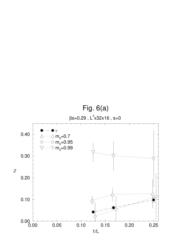
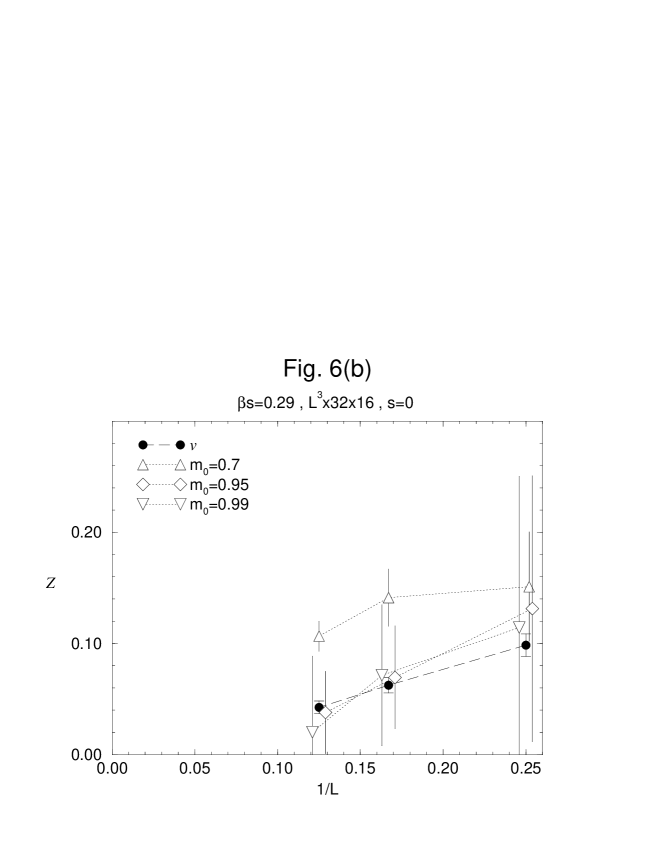
FIG. 6.: (a) $z$(right-handed) and $v$ vs. $1/L$ at $\beta_{s}=0.29$ and (b) $z$(left-handed) and $v$ vs. $1/L$ at $\beta_{s}=0.29$. on $L^{3}\times 32\times 16$ lattices with $L=$4, 6 and 8 at $m_{0}=0.7$ (up triangles), $0.95$ (diamonds) and $0.99$ (down triangles), in the case of putting a source on the domain wall at $s=0$. Solid circles stand for the vacuum expectation value of link variable (:the order parameter).

FIG. 7.: $m_{f}$ vs. $m_{0}$ at $\beta_{s}=0.29$ on $L^{3}\times 32\times 16$ lattices with $L=$4 (circles) , 6 (up triangles) and 8 (down triangles) in the case of putting a source at $s=-1$, for the right-handed fermion (solid symbols) and the left-handed fermion (open symbols). Solid line corresponds to $1+m_{0}$.

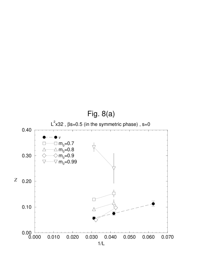
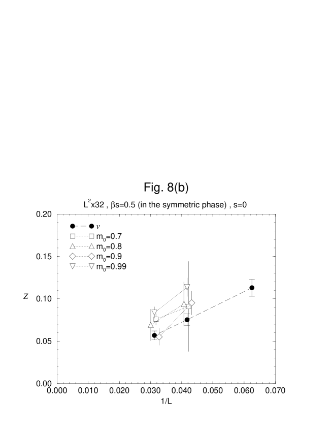
FIG. 8.: (a) $z$(right-handed) and $v$ vs. $1/L$ at $\beta_{s}=0.5$ and (b) $z$(left-handed) and $v$ vs. $1/L$ at $\beta_{s}=0.5$ in the symmetric phase on $L^{2}\times 32$ lattices with $L=$24 and 32 at $m_{0}=0.7$ (squares), $0.8$ (up triangles), $0.9$ (diamonds) and $0.99$ (down triangles), in the case of putting a source on the domain wall at $s=0$. Solid circles stand for the vacuum expectation value of link variable (:the order parameter).

REFERENCES

-
[1]
H. B. Nielsen and M. Ninomiya,
Nucl. Phys. B185, 20 (1981);
erratum: ibid. B195, 541 (1982);
Nucl. Phys. B193, 173 (1981);
Phys. Lett. B105, 219 (1981);
L. H. Karsten, Phys. Lett. B104, 315 (1981). - [2] Y. Shamir, Nucl. Phys. B (Proc. Suppl.)47, 212 (1996) .
-
[3]
D. B. Kaplan,
Phys. Lett. B288, 342 (1992).
For a recent review of domain-wall model, see, K. Jansen, Phys. Rep. 273 ,1 (1996) . - [4] S. Aoki and H. Hirose, Phys. Rev. D49, 2604 (1994).
- [5] S. Aoki and H. Hirose, Phys. Rev. D54, 3471 (1996)
- [6] K. Jansen, Phys. Lett. B288, 348 (1992).
- [7] M. F. L. Golterman, K. Jansen and D.B. Kaplan, Phys. Lett. B301, 219 (1993).
- [8] R. Narayanan and H. Neuberger, Phys. Lett. B302, 62 (1993).
- [9] R. Narayanan and H. Neuberger, Nucl. Phys. B412, 574 (1994).
- [10] M. F. L. Golterman, K. Jansen, D. N. Petcher, and J. C. Vink, Phys. Rev. D49, 1606 (1994).
- [11] M. F. L. Golterman and Y. Shamir, Phys. Rev. D51, 3026 (1995).
-
[12]
R. Narayanan and H. Neuberger,
Nucl. Phys. B443, 305 (1995);
UW-PT-96-04/RU-96-18;
R. Narayanan , H. Neuberger and P. Vranas, Phys. Lett. 353B, 507 (1995);
P. Huet, R. Narayanan and H. Neuberger, Phys. Lett. B380 291 (1995). - [13] S. Randjbar-Daemi and J. Strathdee, Nucl. Phys. B443, 386 (1995); Phys. Lett. B348, 543 (1995); Phys. Rev. D51 , 51 (1995); Nucl. Phys. B461, 305 (1996).
- [14] T. Kawano and Y. Kikukawa, KUNS-1317 .
- [15] C. D. Fosco, hepth/9604050; Int. J. Mod. Phys. A11 3987 (1996); C. D. Fosco and S. Randjbar-Daemi, Phys. Lett. B354 383 (1995).
- [16] Per Ernstom and Ansar Fayyazuddin, NORDITA-95-80 .
- [17] S. Aoki and R. B. Levien, Phys. Rev. D51, 3790 (1995).
- [18] Y. Shamir, Nucl. Phys. B417 167 (1994).
-
[19]
M. F. L. Golterman and Y. Shamir,
Phys. Lett. B353, 84 (1995);
erratum: ibid. B359, 422 (1995);
Nucl. Phys. B (Proc. Suppl.) 47, 603 (1996). - [20] R. Narayanan and H. Neuberger, Phys. Lett. B388, 303 (1995).
- [21] H. Neuberger, RU-95-79 .
- [22] H. Aoki, S. Iso, J. Nishimura, and M. Oshikawa, Mod. Phys. Lett. A9, 1755 (1994).
- [23] C. P. Korthals-Altes, S. Nicolis, and J. Prades, Phys. Lett. B316, 339 (1993).
- [24] S. Aoki and K. Nagai, Phys. Rev. D53, 5058 (1996)