SWAT/102

U(1) Lattice Gauge theory and its Dual

P. K. Coyle^a, I. G. Halliday^b and P. Suranyi^c

^aRacah Institute of Physics, Hebrew University of Jerusalem,
Jerusalem 91904, Israel.
^bDepartment of Physics, University of Wales, Swansea
Singleton Park, Swansea, SA2 8PP, U.K.
^cDepartment of Physics, University of Cincinnati
Cincinnati, Ohio, 45221 U.S.A.

1 Introduction

Duality transformations have provided a useful tool for investigating many theories both in the continuum and on the lattice. The term duality has been used to describe many types of transformation. A common property of these transformations is a mapping from the strong coupling region of one theory into the weak coupling region of its dual. Duality for lattice models was first developed by Kramers and Wannier for the two dimensional Ising model [1] and has since been extended to other more complex lattice models [2, 3]. Here we will use the term duality to refer to the extension of this Kramers and Wannier duality.

This type of transformation is appealing from a practical point of view. Each model has its own set of advantages and disadvantages making simulations difficult for some values of the coupling while they become relatively easy to simulate in other regions.

By relating observables in the original theory to observables in its dual it becomes possible to use the dual model for simulations where the original theory encounters computational difficulties. This is particularly relevant in the weak coupling limit. Here the fields on the original lattice becomes ordered while the dual variables become increasingly disordered.

In this paper we investigate a compact U(1) lattice gauge theory in three dimensions by performing simulations on its dual, the discrete Gaussian model. The duality transformation for this model was first performed by Kogut et.al. [2] and gives a model similar to the Solid on Solid models of surface transitions, but in three dimensions.

2 U(1) and the Discrete Gaussian Model

We consider a compact $U(1)$ gauge theory in 3 dimensions with dynamical variables $U_{i,\mu}$ defined on links, where $i$ labels a site on the lattice and $\mu$ specifies the direction. Each link $U_{i,\mu}$ can be expressed in terms of an angle $-\pi<\theta_{i,\mu}\leq\pi$.

$$U_{i,\mu}=e^{i\theta_{i,\mu}}$$ (1)

with the Wilson action defined as:

$$\beta S=\beta\sum_{\Box}(1-\cos(\theta_{\Box}))$$ (2)

where

$$\theta_{i,\mu\nu} = \theta_{i,\mu}+\theta_{i+\hat{\mu},\nu}-\theta_{i+\hat{\nu},\mu}-\theta_{i,\nu}$$ (3)

$$= \epsilon_{\mu\nu\gamma}\epsilon_{\gamma\alpha\beta}\Delta_{\alpha}\theta_{i,\beta}$$

and

$$\theta_{\Box}=\frac{1}{2}\epsilon_{i,\gamma\mu\nu}\theta_{i,\mu\nu}$$ (4)

The sum in equation (2) is over all sites $i$ and directions $\gamma$ to generate all the plaquettes on the lattice. This gives a partition function:

$$Z=\int_{-\pi}^{\pi}\prod_{j,\mu}d\theta_{j,\mu}e^{-\beta\sum_{\Box}(1-\cos(\theta_{\Box}))}$$ (5)

Although this theory does not experience a phase transition, and thus has no continuum limit, it does possess an interesting topological structure. Through two duality like transformation, this partition function is transformed into the partition function for a coulomb gas of unbound magnetic monopoles plus a free photon field [4, 2, 3, 5, 6]. This identifies the instantons as magnetic monopoles which are exposed by writing the plaquette angle (3) as

$$\theta_{\Box}=\Theta_{\Box}+2\pi n_{\Box}$$ (6)

where $\Theta_{\Box}$ is in the range $-\pi<\Theta_{\Box}<\pi$ and $n_{\Box}=0,\pm 1,\pm 2$. This splits $\theta_{\Box}$ into a continuous part and a part which cannot be written as a gradient. One can therefore define a dual current

$$j_{z-\hat{\mu},\mu}=\frac{1}{2}\epsilon_{\mu\nu\rho}n_{z,\nu\rho}$$ (7)

where $z$ is a site on the dual lattice. The monopoles are then identified by writing

$$\Delta_{\mu}j_{z,\mu} = m_{z}$$ (8)

$$m_{z} = 0,\pm 1,\pm 2,\pm 3$$ (9)

When $m_{z}\neq 0$ there is a monopole/anti-monopole at the (dual) site and the current $j_{z,\mu}$ exposes the Dirac strings connecting monopole anti-monopole pairs. Dirac strings can also form closed loops without any monopoles. With periodic boundary conditions these Dirac strings can form closed loops which wrap around the boundary. The monopoles are physical objects which can be associated with cubes on the lattice however the Dirac strings are gauge dependent so their path can be altered through gauge transformations. Gauge transformations, however, cannot unwind loops which span the boundaries so these loops contribute to a winding number which is gauge invariant. The theory has only a confining ‘plasma’ phase for all values of $\beta$ although the monopoles are found to disappear from the system above $\beta\approx 2.3$ [7, 8].

2.1 The Duality Transformation

The dual model, exposed by Kogut et.al. [2], can be described by the partition function

$$Z=e^{-N\beta}\sum_{\{k\}}\exp\left(\sum_{\Box}\ln[I_{k}(\beta)]\right)\prod_{\Box}\delta(\epsilon_{\mu\beta\alpha}\epsilon_{\alpha\gamma\rho}\Delta_{\beta}k_{i,\gamma\rho})$$ (10)

Where $k_{i,\gamma\rho}$ is the dual variable, $I_{k}(\beta)$ is the modified Bessel function, N is the number of links on the lattice and we have dropped the overall factors of $2\pi$ from the delta functions. As we explicitly sum over all values of $\theta_{i,\mu}$ to generate equation (10) it implicitly includes all possible winding values.

By associating the $k$’s with links on the dual lattice, rather than plaquettes of the original lattice, equation (10) can be interpreted as a spin theory with the interactions on dual links given by

$$k_{z,\alpha}=\frac{1}{2}\epsilon_{\alpha\gamma\rho}k_{i,\gamma\rho}$$ (11)

where $z$ is the site dual to $i$. The constraints on these dual interactions then become

$$\epsilon_{\mu\beta\alpha}\Delta_{\beta}k_{z,\alpha}=0$$ (12)

2.2 Solving the constraints & Boundary Conditions

As equation (12) is just the curl of $k$, these constraints are automatically satisfied by writing $k$ as the gradient of a scalar field. Thus we can express the $k_{z,\alpha}$’s in terms of a (dual) site variable $\phi_{z}$

$$k_{z,\alpha}=\Delta_{\alpha}\phi_{z}$$ (13)

where $\phi\in{{Z}}$. However we must be careful to include all the allowed $k_{z,\alpha}$ configurations. While equation (13) guarantees the constraints are satisfied it does not take into account effects of the periodic boundary conditions.

For an infinite lattice we can write the $k_{z,\alpha}$ as a potential because of Stokes’s Theorem. This works for any closed loops within the lattice. However if we have periodic boundary conditions a contour crossing the boundary an odd number of times forms a loop with no surface associated with it. Stokes’s Theorem therefore doesn’t apply. Writing $k_{z,\alpha}$ as the gradient of $\phi$ forces this loop integral to be zero however the constraints (12) do not impose this restriction on $k_{z,\alpha}$. Therefore while equation (13) is sufficient within the lattice, at the boundary we need a more general prescription for $k_{z,\alpha}$ in order to generate all the allowed configurations.

For the boundary links we can write $k_{z,\alpha}$ as:

$$k_{z,\alpha}=\Delta_{\alpha}\phi_{z}+Q_{z,\alpha}(z)$$ (14)

Using the constraints (12) on $Q$ gives

$$\epsilon_{\mu\nu\sigma}\Delta_{\nu}(\Delta_{\sigma}\phi_{z}+Q_{z,\sigma}(z))=0$$ (15)

Thus

$$\Delta_{\nu}Q_{z,\sigma}(z)=0$$ (16)

for $\sigma\neq\nu$, so $Q_{\sigma}$ cannot change across each plane perpendicular to $\sigma$ leaving only three extra degrees of freedom $Q_{i},Q_{j}$ and $Q_{k}$. Now if we consider the line integral for a loop $C$ which crosses the $\mu$ boundary once we get

$$\int_{C}k_{\mu}\cdot dl = \sum_{C}k_{\mu}$$ (17)

$$= Q_{\mu}$$ (18)

These extra parameters therefore allow the fields $\phi$ to differ by $Q$ across the boundary without any cost to the action. This winding is the three dimensional extension of the ‘step free energy’ often introduced for two dimensional SOS models [9]. In two dimensions the cyclic boundary conditions are related to pinning the boundary of the surface. The extra ‘step free energy’, Q is introduced to remove this pinning constraint in the hope of improved statistics.

The minimum requirement for generating all the interactions satisfying the constraints in (10) with periodic boundary conditions is therefore

$$k_{z,\mu}=\Delta_{\mu}\phi_{z}+Q_{\mu}$$ (19)

for links on the boundary and

$$k_{z,\mu}=\Delta_{\mu}\phi_{z}$$ (20)

for all other points.

As the step free energies $Q$ are related to the boundary conditions they become less important as the lattice size is increased. When $\beta$ is small the fields are predominantly at one level and, using the language of SOS models, the system is ‘smooth’. Non-zero $Q$ values therefore increase the energy for every link on the boundary and are subsequently suppressed by a factor proportional to the lattice size squared. At large $\beta$ the system becomes ‘rough’ with a ‘thickness’ that increases with $\beta$ and with the lattice size. In this region changing $Q$ will, on average, decrease the energy for as many interactions as it increases it, provided $Q$ is less than the thickness. Correlation functions are unaffected by these changes in $Q$ and with only three winding parameters, compared with the $L^{3}$ site variables, fixing $Q$ should not influence correlation function measurements, even for modest lattice sizes. We therefore set $Q=0$ below although it can be replaced at any time if desired.

$$Z=e^{-N\beta}\sum^{\infty}_{\{\phi\}=-\infty}\exp(\sum_{l_{d}}\ln[I_{(\Delta_{\rho}\phi_{z})}(\beta)])$$ (21)

Where we have a sum over configurations of site variables $\phi_{z}$ with an interaction defined on links $k_{\rho}=\Delta_{\rho}\phi_{z}$.

2.3 The Weak Coupling limit

By considering the weak coupling limit Kogut et.al were able to simplify (21) considerably. In this limit the partition function reduces to a discrete Gaussian model.

$$\ln(I_{n}(\beta))\approx-\frac{n^{2}}{2\beta}+\beta-\ln(2\pi\beta^{\frac{1}{2}})$$ (22)

To improve this approximation we can systematically add higher order powers of $n$. This approximation is equivalent to using the periodic Gaussian or Villain action [10]. The $\beta$ on the right had side of equation (22) can therefore be identified with $\beta_{v}$, the Villain beta. In his original paper Villain determined an approximate relationship between the cosine beta, $\beta$ and $\beta_{v}$.

$$\beta_{v}(\beta)=\left[2\ln\left(\frac{I_{0}(\beta)}{I_{1}(\beta)}\right)\right]^{-1}$$ (23)

Where $I_{0}(\beta)$ and $I_{1}(\beta)$ are modified Bessel functions. This relationship is found through matching the first terms in the expansion of the cosine and Villain Boltzmann factors and is therefore equivalent to adding extra terms in equation (22). A good approximation to the partition function is therefore

$$Z=\sum_{\{\phi\}}\exp\left(\sum_{\rho,j}\ln[\frac{I_{0}(\beta)}{I_{1}(\beta)}](\Delta_{\rho}\phi_{j})^{2}\right)$$ (24)

2.4 Wilson loops

In the weak coupling limit Wilson loops become correlation functions of the dual variables. Defining a loop W(J) where the current $J_{i,\mu}$ defines the contour with $J_{i,\mu}$ given by:

$$J_{i,\mu}=\left\{\begin{array}[]{l}+1\mbox{ if link }i\rightarrow i+\mu\mbox{ is in $C$. }\\ -1\mbox{ if link }i+\mu\rightarrow i\mbox{ is in $C$. }\\ 0\mbox{ otherwise }\end{array}\right.$$ (25)

The expectation value of this loop is then

$$W(J)=\frac{1}{Z}\prod\int_{-\pi}^{\pi}e^{-\beta_{v}(\sum_{i,\Box}1-\cos(\theta_{i,\Box})+i\sum_{i,\mu}\theta_{i,\mu}J_{i,\mu})}$$ (26)

After the duality transformation, in the weak coupling limit, this become

$$W(J)=\frac{1}{Z}\sum_{\{\phi\}}e^{\frac{1}{2\beta_{v}}k^{2}_{\mu\nu}(\phi,S(J))}$$ (27)

where in order to satisfy the new constraints $k_{\mu\nu}$ is written as

$$k_{\mu\nu}=S_{\mu\nu}+\epsilon_{\mu\nu\lambda}\Delta_{\lambda}\phi_{i}$$ (28)

Where $S_{\Box}=1$ for an oriented surface with $J_{\rho}\neq 0$ as its boundary and zero everywhere else. Expanding the exponential for the extra terms due to $S_{\Box}=1$ leaves

$$W(J)=\frac{1}{Z}\sum_{\{\phi\}}e^{\frac{A}{2\beta_{v}}}\left(1+\frac{(\sum_{l_{d}}l_{i,\rho}\Delta_{\rho}\phi_{i})^{2}}{2\beta_{v}^{2}}+\cdots\right)e^{\frac{1}{2\beta_{v}}\sum_{l_{d}}(\Delta\phi_{i,\rho})^{2}}$$ (29)

where $A$ is the number of plaquettes in the surface $S_{\mu\nu}$ and the sum in each term is over the dual links $l_{\rho}=\frac{1}{2}\epsilon_{\rho\mu\nu}S_{\mu\nu}$ which penetrate the surface $S_{\mu\nu}$. Thus for the $1\times 1$ Wilson loop, to order $\frac{1}{\beta_{v}^{2}}$

$$W(\Box)=e^{-\frac{1}{2\beta_{v}}}\left(1+{\frac{1}{\beta_{v}^{2}}}(\langle\phi_{i}^{2}-{\bar{\phi_{i}}}^{2}\rangle-\langle\phi\phi_{i+1}-{\bar{\phi}}^{2}\rangle)\right)$$ (30)

where $\bar{\phi}=\langle\phi\rangle$.

3 Measurements

In order to judge how useful the discrete Gaussian model is from a numerical perspective we also performed simulations using a U(1) lattice measuring the $1\times 1$ Wilson loop directly. We considered lattices of size $8^{3}$ and $16^{3}$ with periodic boundary conditions. We used a standard metropolis algorithm and discarded the first 2,000 updates, where each update constituted a Metropolis hit for all links in the lattice. 50,000 updates were then performed taking measurements after every update. The simulations were performed on DEC Alpha 3400AXP workstations where, for a $16^{3}$ lattice, each update took $0.212\pm 0.001$ seconds.

Before attempting accurate calculations for $U(1)$ observables using the discrete Gaussian correlation functions we first checked that these measurements were insensitive to the step free energies.

We compared simulations where the step free energy $Q_{\alpha}$ was fixed at zero, with simulations where $Q_{\alpha}$ was dynamically updated through a metropolis procedure before each measurements. We found that $\langle|Q|\rangle$ remained zero for $\beta$ below $\approx 2.2$ while above it increased monotonically. Measurements of the correlation functions however, were the same, within errorbars, for both static and dynamically varying step free energies. We therefore set $Q_{\alpha}=0$ for the remainder of our simulations.

Simulations for the Discrete Gaussian model were performed on $8^{3}$ and $16^{3}$ lattices. Again, in order to compare like with like, we implemented a metropolis algorithm with each update consisting of a metropolis hit on each site of the lattice. We ran 210,000 updates and discarded the first 10,000. Again we used DEC Alpha 3400AXP workstations and each update took $0.033\pm 0.001$ seconds for a $16^{3}$ lattice, almost 6.5 times faster than U(1). We measured the correlation functions after each update and used these to estimate the U(1) $1\times 1$ Wilson loop through equation 30. The results are shown in figure 1 together with the strong and weak coupling expansions for the U(1) model [11, 12].

$$\langle\Box\rangle \approx \frac{1}{3\beta}+\cdots\qquad\qquad\qquad\mbox{ to order }O(\frac{1}{\beta^{2}})$$ (31)

$$\approx \frac{\beta}{2}+\frac{\beta^{3}}{12}+\cdots\qquad\mbox{ to order }O(\beta^{3})$$ (32)

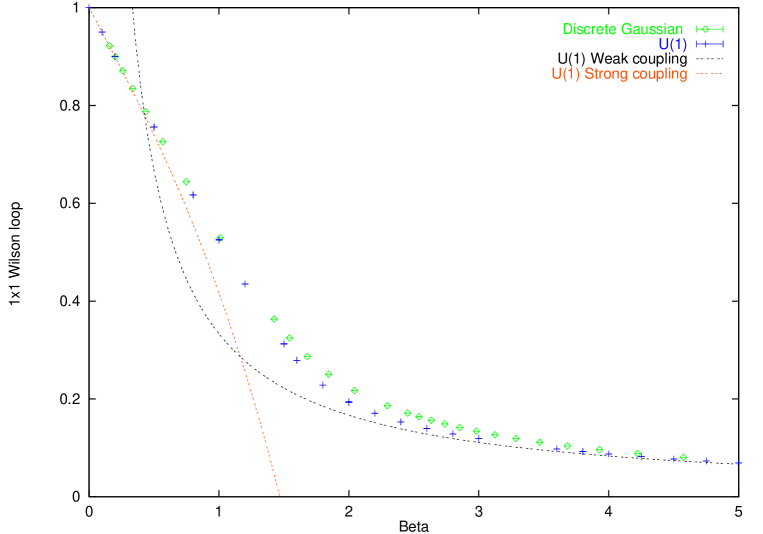
Figure 1: $\langle\Box\rangle$ from U(1) and Discrete Gaussian simulations

4 Errors and Efficiency

In order to estimate the errors we split the raw data into bins of size 2 to 500. We used this blocking to measure the overall errors and calculate auto-correlation times $\tau$. We also checked that $\tau$ calculated in this way was the same as $\tau_{exp}$ calculated from an exponential fit to the auto-correlation functions.

We used $\tau$ to split the errors in the calculation into two parts, an autocorrelation ($\tau$) component and a standard error ($\sigma$) component. The total sample error,$\sigma_{s}$ for a given simulation is then approximately

$$\sigma_{s}=\sigma\sqrt{\frac{2\tau}{N}}$$ (33)

where N is the sample size. The autocorrelation times measure the efficiency of the update algorithm and are shown in figure 2a while $\sigma$ measures the statistical errors for each independent measurement and depends only on the model. These are shown in figure 2b where again we have used blocking to estimated errors.

For the U(1) lattice the measurement error decreases significantly above $\beta\approx 2$. This is what we expect from the topological picture. At large $\beta$ the monopoles condense out and the effective number of degrees of freedom therefore reduces considerably. Autocorrelations also increase around $\beta\approx 2$ signaling the emergence of extended objects. These are the monopoles which become important as the temperature decreases before they disappear from the system. Above $\beta\approx 2$ the autocorrelation times fall when there are no monopoles. The autocorrelations remain short for large $\beta$.

Figure 2: a) U1 Autocorrelations Errors (algorithm error) b) U1 Standard Errors

For the Discrete Gaussian model autocorrelation times also increase around $\beta\approx 2$, however, they remain high as $\beta$ increases. At small $\beta$ the lattice is smooth but above $\beta\approx 2$ it becomes rough and the local algorithm slows down. This is different to the usual slowing down in spin models which occurs at low temperature. Here the large scale objects of the dual model appear at hight temperature as the dual model becomes more disordered and the ‘thickness’ increases. This causes the local metropolis algorithm we used to have difficulty updating configurations. This suggest that a cluster algorithm may be effective at improving these simulations. A Solid On Solid algorithm has been developed for the two dimensional discrete Gaussian model by Evertz et al. [13]. This algorithm should be directly applicable to the three dimensional model although, to our knowledge, it has not been tested on a three dimensional lattice. The measurement error for the Discrete Gaussian model experiences a peak around $\beta=2$ but most of this structure is generated by the transformation in equation (30).

Figure 2 shows that both the auto-correlation times and the errors in each independent measurement are worse for the dual model for most values of beta. However the dual simulations ran over six times faster than the equivalent U(1) calculations so in order to compare the overall efficiency we need to consider simulations requiring the same amount of CPU time. Using equation (33) we can scale the results to estimate the errors for simulations taking the same amount of computer time. This is shown in figure 3. The dual model therefore only becomes more efficient for $\beta<2$. However as the transformation utilizes the weak coupling limit the dual model is expected to be most accurate for large $\beta$.

Figure 3: Total error in $\langle S_{U1}\rangle$ for a given CPU time. Errors are estimated using blocking

5 Conclusion

The main advantage of the dual model is the speed of its updates compared to the equivalent U(1) lattice. This increase in speed comes from using integer variables and a lack of local gauge invariance. This advantage however is destroyed by the large auto-correlation times generated by the local metropolis algorithm. The Discrete Gaussian model has the unusual characteristic of generating large-scale structures when the fields become disordered. This is the region where the U(1) system is at weak coupling and ordered and is when the transformation is most accurate.

Cluster algorithms exist for both the U(1) and Discrete Gaussian models. And the Discrete Gaussian simulations would have benefited dramatically from an efficient algorithm. However our main concern was to study the transformation as a tool to improve the simulations. We were therefore careful to consider both theories on an equal footing. Here we have seen that by studying the dual model the characteristics of the simulations can be changes significantly. However whether this is of any practical use depends on the form of the dual model and the update algorithms available in each case.

For U(1) it is unfortunate that the weak coupling region corresponds to the ‘rough’ region of the dual model. This means that the disadvantages of both models occur when the duality transformation is most accurate. The opportunity to utilize better statistical properties of the dual theory therefore does not occur and the only gains produced are from the smaller configuration space. This is not always the case. Recently M.Zach et.al [14] have shown that in four dimensions, the U(1) dual model can be significantly more efficient than direct U(1) simulations.

The recent progress in duality transformations for non-Abelian models [15] allows for a similar study of more complex dual theories. These more realistic models transform to dual theories without their large scale excitations at high dual temperatures. They should therefore not encounter the simulation difficulties experienced by the discrete Gaussian model. For U(1) in three dimensions, simulations are relatively efficient and leave little opportunity for improvement. The increased complexity and difficulties experienced with non-abilian models allows more scope for improvement than this simple U(1) case.

References

- [1] H.A.Kramers and G.H.Wannier. Phys. Rev, 60:252, 1941.
- [2] J.B.Kogut, T.Banks, and R.Myerson. Phase transitions in abelian lattice gauge theories. Nucl.Phys., B129:493, 1977.
- [3] R.Savit. Duality in field theory and statistical systems. Rev. Mod. Phys., 52:453–497, 1980.
- [4] A.M.Polyakov. Quark confinement and topology of gauge theories. Nucl.Phys., B120:429, 1975.
- [5] R.Savit. Topological excitations in u(1)-invariant theories. Phys. Rev. Lett., 39(2):55–58, 1977.
- [6] R.Savit. Vortices and the low-temperature structure of the x-y model. Phys. Rev, B17(3):1340–1350, 1978.
- [7] A. Hulsebos and P. Ueberholz. Topological updating schemes: A case study in 3-d u(1). Nuclear Physics B (Proc. Suppl.), 42:873–875, 1995.
- [8] M.I. Polikarpov, K.Yee, and M.A. Zubkov. Compact qed in landau gauge: A lattice gauge fixing case study. Phys.Rev., D48:3377–3382, 1993.
- [9] C.Domb and J.L.Lebowitz, editors. Phase Transitions and Critical Phenomena. Academic Press, 1986.
- [10] J.Villain. J. of Phys., 34:581, 1975.
- [11] H.J.Rothe. Lattice Gauge Theories, An Introduction. World Scientific, 1992.
- [12] M.Creutz. Quarks, gluons and lattices. Cambridge University Press, 1983.
- [13] H.G.Evertz, M.Hasenbusch, M.Marcu K.Pinn, and S.Solomon. Stochastic cluster algorithms for discrete gaussian (sos) models. Phys.Lett., B254:185–191, 1991.
- [14] M. Zach, M. Faber, and P. Skala. Field strength and monopoles in dual u(1) lattice gauge theory. hep-lat/9608009.
- [15] I.G.Halliday and P.Suranyi. Duals of nonabelian gauge theories in d dimensions. Phys.Lett., B350:189–196, 1995.