UTHEP-348

UTCCP-P-19

February, 1997

Scaling in SU(3) Pure Gauge Theory
with a Renormalization Group
Improved Action

Y. Iwasaki,^a,b K. Kanaya,^a,b T. Kaneko,^a and T. Yoshié^a,b

^a Institute of Physics, University of Tsukuba, Ibaraki 305, Japan
^b Center for Computational Physics, University of Tsukuba,
Ibaraki 305, Japan

We study the scaling properties of the static quark potential and the ratio of the critical temperature $T_{c}$ to the square root of the string tension $\sigma$ in the SU(3) pure gauge theory using a renormalization group improved action. We first determine the critical coupling $\beta_{c}$ on lattices with temporal extension $N_{t}=3$, 4, and 6, and then calculate the static quark potential at the critical couplings on lattices at zero temperature. We note that the static quark potentials obtained are rotationally invariant with errors of at most 1 – 2 % in all the three cases, and that the potential $V(R)$ in physical units scales in the whole region of $R$ investigated. The values of $T_{c}/\sqrt{\sigma}$ for the three cases in the infinite volume limit are identical within errors. We estimate the value in the continuum limit to be $T_{c}/\sqrt{\sigma}=0.656(4)$, which is slightly larger than the value in the continuum limit from the one-plaquette action, 0.629(3).

1 Introduction

In numerical studies of lattice QCD, it is important to control and reduce finite lattice spacing effects. Several improved actions have been proposed for this purpose and some of them have been tested for the scaling behavior of the critical temperature $T_{c}$ of the finite temperature deconfining transition [1, 2, 3, 4, 5].

In this work we study the scaling properties of the static quark potential and the ratio of the critical temperature to the square root of the string tension $\sigma$, $T_{c}/\sqrt{\sigma}$, in the SU(3) pure gauge theory, using a renormalization group (RG) improved action [6]:

$$S_{g}^{\rm IM}={\beta\over 6}\,\{c_{0}\sum(1\times 1{\rm\ loop})+c_{1}\sum(1\times 2{\rm\ loop})\}$$ (1)

with $c_{1}=-0.331$ and $c_{0}=1-8c_{1}$, where $\beta=6/g^{2}$ ($g$ is the gauge coupling). In Eq.(1), the loops are defined by the trace of ordered product of link variables and each oriented loop appears once in the sum.

This paper is organized as follows. First we determine the critical coupling $\beta_{c}$’s for the finite temperature deconfining phase transition on $9^{3}\times 3$, $12^{3}\times 4$ and $18^{3}\times 6$ lattices in Sec. 2. We also perform simulations on $12^{3}\times 3$, $15^{3}\times 3$, $16^{3}\times 4$, and $20^{3}\times 4$ lattices for a finite size scaling study. Then the quark potentials at the three $\beta_{c}$’s are calculated from smeared Wilson loops on $9^{3}\times 18$, $12^{3}\times 24$ and $18^{3}\times 36$ lattices, respectively, in Sec. 3. The string tension is extracted from the quark potential assuming that the potential takes a form of a sum of a Coulomb term and a linearly rising potential. In Sec. 4, scaling behavior of the quark potential and that of the ratio $T_{c}/\sqrt{\sigma}$ are examined. Finally, the value of the ratio $T_{c}/\sqrt{\sigma}$ in the continuum limit and in the infinite volume limit is estimated.

2 Critical coupling $\beta_{c}$

In order to determine the critical coupling $\beta_{c}$ for the finite temperature phase transition, we perform simulations on $9^{3}\times 3$, $12^{3}\times 4$ and $18^{3}\times 6$ lattices. The critical temperature $T_{c}$ is given by $T_{c}=1/(aN_{t})$, where $N_{t}$ is the linear extension of the lattice in the temporal direction and $a$ is the lattice spacing at the critical coupling. Note that the physical spatial volumes are identical for all the three cases, $(N_{s}a)^{3}=(3N_{t}a)^{3}=(3/T_{c})^{3}$, where $N_{s}$ is the linear extension of the lattice in the spatial direction.

We also perform simulations on lattices with different spatial volumes for an estimation of the infinite volume limit of $\beta_{c}$ using finite size scaling analyses. The previous results for the case of the standard one-plaquette action on spatially large lattices [7, 8] indicate that extrapolations from small lattices with the aspect ratio $N_{s}/N_{t}\leq 3$ result in sizable systematic errors in the values of $\beta_{c}$ in the infinite volume limit. Therefore, we restrict ourselves to lattices $N_{s}/N_{t}\geq 3$ in this paper. We perform simulations on $12^{3}\times 3$, $15^{3}\times 3$, $16^{3}\times 4$, and $20^{3}\times 4$ lattices for finite size analyses. We reserve finite size study of $N_{t}=6$ lattices for future investigation.

Gauge fields are updated by a Cabibbo-Marinari-Okawa pseudo heat bath algorithm with 8 hits both for the simulations at finite temperatures and at zero temperature discussed in the next section. The simulation parameters are compiled in Table 1. We measure Wilson loops and Polyakov line every 10 sweeps. Their expectation values are summarized in Tables 2 - 8. (For the deconfinement fraction, see below.)

The values of the critical coupling $\beta_{c}$ are determined as the peak location of the susceptibility $\chi$ of the Z(3) rotated Polyakov line $\Omega$:

$$\chi=\langle\;\Omega^{2}\;\rangle-\langle\;\Omega\;\rangle^{2}$$ (2)

$$\Omega=\left\{\begin{array}[]{lll}\mbox{Re}\;P\exp\left[-\frac{2}{3}\pi\right]&;\;\;\;\mbox{arg}P\in\left[\pi/3,\pi\right)\\ \mbox{Re}\;P&;\;\;\;\mbox{arg}P\in\left[-\pi/3,\pi/3\right)\\ \mbox{Re}\;P\exp\left[\frac{2}{3}\pi\right]&;\;\;\;\mbox{arg}P\in\left[-\pi,-\pi/3\right){{}_{,}}\end{array}\right.$$ (3)

where $P$ is the spatially averaged timelike Polyakov line

$$P={\frac{1}{N_{s}^{3}}}\sum_{\bf{x}}\frac{1}{3}\makebox{Tr}\left[\prod_{t=1}^{N_{t}}U{{}_{4}}\left({\bf{x}},t\right)\right]_{.}$$ (4)

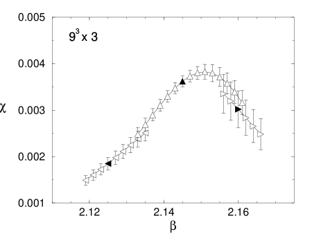
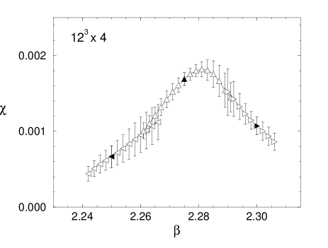
Figure 1: Susceptibility $\chi$ of the Z(3) rotated Polyakov line $\Omega$ on the $9{{}^{3}}{\times}3$, $12{{}^{3}}{\times}4$ and $18{{}^{3}}{\times}6$ lattices. Each curve is obtained from the data at the simulation point indicated by the filled symbol using the spectral density method. Errors for open symbols are computed by a jack-knife method combined with the spectral density method.

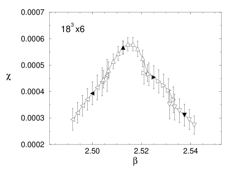
Figure 1: continued

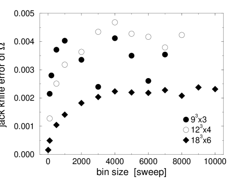
Figure 2: Bin size dependence of the jack knife error of $\Omega$.

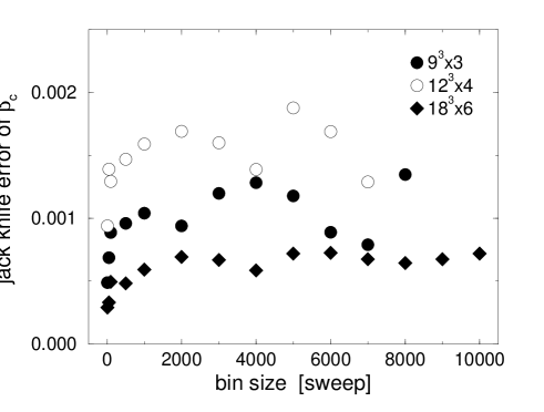
Figure 3: Bin size dependence of the jack knife error of $\beta_{c}$.

The results of the susceptibility calculated using the spectral density method [9] on the $9^{3}\times 3$, $12^{3}\times 4$, and $18^{3}\times 6$ lattices are shown in Fig. 1. The results obtained at several simulation points are consistent with each other within the errors and form a clear peak structure. The value of $\beta_{c}$ is determined from the data at the $\beta$ which is the closest to $\beta_{c}$. The errors are estimated using a single-elimination jack knife method. The bin size in the jack knife method is determined by investigating the bin size dependence of the errors of $\Omega$, shown in Fig. 2. We note that the jack-knife errors of $\beta_{c}$’s are stable for the bin size larger than those adopted, as shown in Fig. 3. The values of $\beta_{c}$’s and their jack-knife errors are summarized in Table 9.

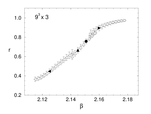
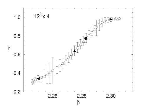
Figure 4: Deconfinement fraction $r$ on the $9{{}^{3}}{\times}3$, $12{{}^{3}}{\times}4$ and $18{{}^{3}}{\times}6$ lattices. Each curve is obtained from the data at the simulation point indicated by filled triangles. The values of $\beta_{c}$ determined from the peak position of the susceptibility are shown by filled circles.

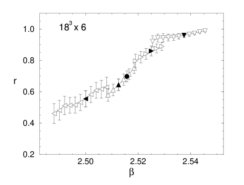
Figure 4: continued

There are several alternative definitions of $\beta_{c}$ on finite lattices. A popular method is to measure the “deconfinement fraction” $r$ given by $r=(3p-1)/2$ where $p$ is the probability such that $\arg P\in(-\pi/9,\pi/9)$, $(2\pi/3-\pi/9,2\pi/3+\pi/9)$, or $(-2\pi/3-\pi/9,-2\pi/3+\pi/9)$, and to define $\beta_{c}$ as a point where $r$ takes a given value. Our results of $r$ as a function of $\beta$ for the case of the aspect ratio $N_{s}/N_{t}=3$ are shown in Fig. 4. See also Tables 2-9. We find that the deconfinement fraction $r$ is approximately 0.75 at $\beta_{c}$ determined from the peak location of the susceptibility, as summarized in Table 9. We note that this fact for the deconfinement fraction is also realized in data [8] obtained for the standard one-plaquette action on large lattices with high statistics (see Table 10). The condition $r=3/4$ is the criterion taken in Ref. [10] for the determination of $\beta_{c}$. (See also the discussions in Refs. [11, 12].) However, the volume dependence of the corrections of $\beta_{c}$ to the infinite volume limit is not known in this case. On the other hand, a scaling relation is well established for the $\beta_{c}$ determined from the peak location of the susceptibility. Therefore, we concentrate on $\beta_{c}$ determined from the peak location of the susceptibility for finite size scaling analyses.

In the following, we denote the $\beta_{c}$ on the $9^{3}\times 3$, $12^{3}\times 4$, and $18^{3}\times 6$ lattices as $\beta_{c}(9^{3}\times 3)$, $\beta_{c}(12^{3}\times 4)$, and $\beta_{c}(18^{3}\times 6)$, respectively.

3 String tension

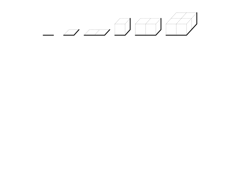
Figure 5: Units of spatial paths of Wilson loops.

We evaluate the string tensions at $\beta=\beta_{c}(9^{3}\times 3)$, $\beta_{c}(12^{3}\times 4)$, and $\beta_{c}(18^{3}\times 6)$ on lattices at zero temperature: $9^{3}\times 18$, $12^{3}\times 24$, and $18^{3}\times 36$ lattices, respectively. Note that the spatial sizes of the lattice are the same as those for the finite temperature simulations in all the three cases. The ratio $N_{t}/N_{s}$ is also fixed to 2. The simulation parameters are summarized in Table 11. After thermalization sweeps, we measure Wilson loops every 200 sweeps. The spatial paths of the loops are formed by connecting one of the spatial vectors shown in Fig. 5.

In order to extract the ground state contribution to the potential, we adopt the smearing technique proposed in Ref.[14]: Each spatial link $U$ is replaced with an SU(3) matrix $U_{\rm new}$ which maximizes $\mbox{ReTr}\left[FU_{\rm new}\right]$, with $F$ being the sum of the spatial staple products of link variables around $U$. We perform this procedure up to 10, 30 and 40 steps on the $9^{3}\times 18$, $12^{3}\times 24$ and $18^{3}\times 36$ lattices, respectively. Measurements are carried out every smearing step on the $9^{3}\times 18$ and every 2 smearing steps on the other lattices. With this smoothing procedure the behavior of the effective mass

$$m_{\rm eff}=\mbox{log}\left[W(R,T)/W(R,T+1)\right]$$ (5)

in terms of $T$ is much improved, especially for large $R$ as shown in Fig. 6.

In the following, we discuss separately the results of the potential $V(R)$ at $\beta_{c}$ for $N_{t}=4$ and 6, and that for $N_{t}=3$, because in the former case we are able to extract the coefficient of the Coulomb term by a straightforward fitting procedure with examining the stability of the fit, while in the latter case it is hard to fix it solely from the data due to a small number of the data points caused by the coarseness of the lattice at $\beta_{c}(9^{3}\times 3)$ (see discussions below).

3.1 Results at $\beta_{c}(12{{}^{3}}\times 4)$ and $\beta_{c}(18{{}^{3}}\times 6)$

The potential $V(R)$ and the overlap function $C(R)$ are extracted by a fully correlated fit of Wilson loops to the form

$$W(R,T)=C(R){\cdot}\mbox{ exp}\left[-V(R){\cdot}T\right].$$ (6)

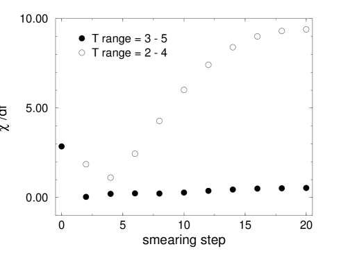
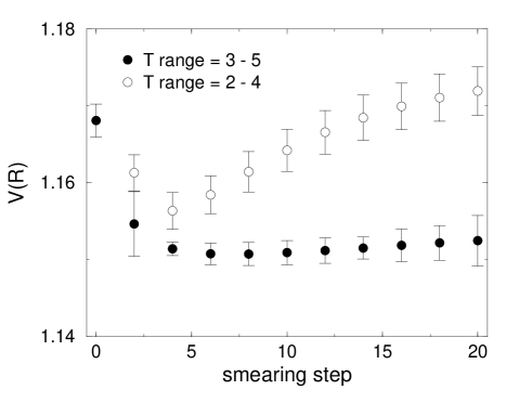
Figure 7: Smearing step dependence of $\chi{{}^{2}}/df$ and $V(R)$ at $R=4.0$ on the $12^{3}\times 24$ lattice.

The fitting range is determined by examining carefully $\chi{{}^{2}}/df$ and stability of $V(R)$ against the smearing step. Fig. 7 shows the results of $\chi{{}^{2}}/df$ and $V(R)$ versus the smearing step at $R=4.0$ for the case of $\beta_{c}(12{{}^{3}}\times 4)$. When we take the fitting range $T=3-5$, we find that $\chi{{}^{2}}/df$ $<$$\sim$ 1 and $V(R)$ is quite stable after four smearing steps, while the choice of the fitting range $T=2-4$ leads to $\chi{{}^{2}}/df$ much larger than 1 and a significant variation of $V(R)$ against the smearing step. We find that the choice of the fitting range $T=3-5$ leads to reasonable $\chi^{2}/df$ and stability of $V(R)$ against the smearing step for all $R$ except $2\sqrt{6}$ (where $\chi^{2}/df$ takes a little large value $\sim 2.5$, though the stability is satisfied). This stability implies that the contamination from excited states is negligible small. Therefore, we take the fitting range $T=3-5$ for the data at $\beta_{c}(12{{}^{3}}\times 4)$. The $T$ range $4-7$ at $\beta_{c}(18{{}^{3}}\times 6)$ is determined in a similar way.

We determine the optimum number of smearing steps for each $R$ in such a way that $C(R)$ takes the largest value under the condition $C(R)\leq 1$ which we call the “optimum smearing step”. We note that $\chi^{2}/df$ is stable ($<$$\sim$ 1) against a variation of the smearing step when $C(R)\simeq 1$. The optimum smearing steps thus determined are about 8 at $\beta_{c}(12{{}^{3}}\times 4)$, and are distributed from $12$ to $40$ at $\beta_{c}(18{{}^{3}}\times 6)$ (see Tables 12 and 13). We take the value of $V(R)$ at the optimum smearing step. The systematic error due to the choice of the smearing step is much smaller than the statistical error, because the value of $V(R)$ is stable against the smearing step as mentioned above, and therefore we neglect it in the following.

The values for $V(R)$ are summarized in Tables 12 and 13. Statistical errors are estimated by the jack-knife method with bin size 1. Note that measurements are performed every 200 sweeps. We confirm that the errors are quite stable against the bin size.

The string tension is determined by fitting $V(R)$ to the rotationally invariant ansatz

$$V(R)=V_{0}-{\alpha\over R}+{\sigma_{\rm lat}}R,$$ (7)

where $\sigma_{\rm lat}=\sigma a^{2}$ is the string tension in lattice units. We take into account the correlations among $V(R)$ at different $R$ using the error matrix derived from those for $W(R,T)$. The fitting ranges we take are

$$\begin{array}[]{ll}R=\sqrt{6}\;-\;4\sqrt{2}&(12{{}^{3}}{\times}24),\\ R=2\sqrt{3}\;-\;4\sqrt{5}&(18{{}^{3}}{\times}36).\\ \end{array}$$ (8)

These ranges ($R_{\rm min}$ – $R_{\rm max}$) are determined by investigating the stability of fits and the value of $\chi^{2}/df$ as explained in the following. As we increase $R_{\rm min}$, instability of the fit first appears in the result of $\alpha$, while the results of $V_{0}$ and $\sigma_{\rm lat}$ are stable. The error of $\alpha$ becomes abruptly large as $R_{\rm min}$ increases: e.g. at $\beta_{c}(12{{}^{3}}\times 4)$ with $R_{\rm max}=4\sqrt{2}$ fixed, $\alpha=0.332(11),0.295(14),0.154(101)$, and -0.040(121) for $R_{\rm min}=\sqrt{5}$, $\sqrt{6}$, $2\sqrt{2}$, and 3.0, respectively. Therefore, we restrict candidates for $R_{\rm min}$ to those for which the error of $\alpha$ is less than 50% of the central value. We find that $\chi^{2}/df$ is stable and $\sim 1$ for $5\leq R_{\max}<6$ [$7\leq R_{\max}<9$ ] at $\beta_{c}(12{{}^{3}}\times 4)$ [$\beta_{c}(18{{}^{3}}\times 6)$] which we take as the candidates for $R_{\rm max}$. The fitting range is determined by the condition that $\chi^{2}/df$ takes a value nearest to 1 in all the combinations of the candidates for $R_{\rm min}$ and $R_{\rm max}$. The values of $\chi^{2}/df$ are 1.5 and 1.2 at $\beta_{c}(12{{}^{3}}\times 4)$ and $\beta_{c}(18{{}^{3}}\times 6)$, respectively, for the $R_{\rm min}$ and $R_{\rm max}$ adopted. We have checked that the results of $\alpha$ and $\sigma_{\rm lat}$ are stable for all candidates of $(R_{\rm min},R_{\rm max})$ which satisfy

$$\begin{array}[]{ll}2.0\leq R_{\rm min}\leq\sqrt{6},\;\;\;\;\;5.0\leq R_{\rm max}\leq 6.0&(12^{3}\times 24)\\ 3.0\leq R_{\rm min}\leq 3\sqrt{2},\;\;\;7.0\leq R_{\rm max}\leq 9.0&(18^{3}\times 36).\\ \end{array}$$ (9)

Note that the changes of the fitting ranges of $R$ at these two $\beta$’s are consistent with the change of the scale between $\beta=\beta_{c}(12{{}^{3}}{\times}4)$ and $\beta_{c}(18{{}^{3}}{\times}6)$, that is, the ratio of 4 to 6.

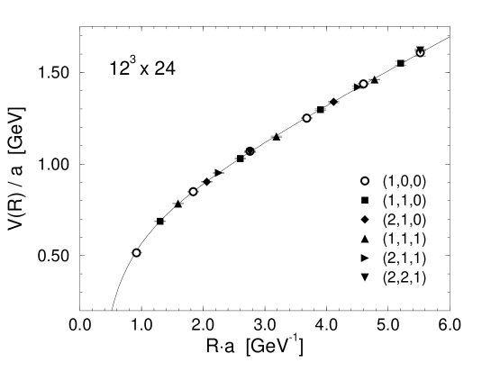
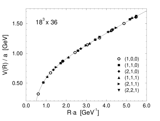
Figure 8: Data for the potential and its fitting curves on the $12{{}^{3}}{\times}24$ and $18{{}^{3}}{\times}36$ lattices. The values of $a$ are determined from $\sigma=(420\mbox{MeV})^{2}$. The legends for the symbols represent the units of spatial paths of Wilson loops shown in Fig. 5.

The results of $V_{0}$, $\alpha$, $\sigma_{\rm lat}$, and their jack knife errors are summarized in Table 14. The values of $V(R)$ are plotted in Fig. 8, where different symbols correspond to different units of spatial path of Wilson loops. The values of $V(R)$ obtained from six types of Wilson loops are excellently fitted to the rotationally invariant form, Eq.(7). The deviations of the data at $\beta_{c}({12^{3}}\times 4)$ from the fitted curve are less than 2% and the average of them is about 0.4%. For the data at $\beta_{c}({18^{3}}\times 6)$, the deviations are at most 1% with the average about 0.3%.

We note that the results of $\alpha$ are consistent with a constant within the errors. The resulting $\alpha\simeq 0.296$ is slightly larger than $\pi/12\simeq 0.262$ derived in a string model [15]. We also perform fits with the value of $\alpha$ fixed to $\pi/12$. Then the values obtained are $\sigma_{\rm lat}=0.1527(14)$ and $0.0667(6)$ at $\beta_{c}(12{{}^{3}}\times 4)$ and $\beta_{c}(18{{}^{3}}\times 6)$, respectively. The values for the ratio $T_{c}/\sqrt{\sigma}$ using these results are consistent with our final results using the values in Table 14 within one standard deviation.

3.2 Results at $\beta_{c}(9{{}^{3}}\times 3)$

We obtain the potential $V(R)$ at $\beta_{c}(9^{3}\times 3)$ by fitting $W(R,T)$ to the form Eq.(6) with the fitting range $T=2\;-4\;$. The fits with this fitting range have desirable properties similar to those at the other two $\beta_{c}$’s discussed in the preceding subsection; reasonable $\chi{{}^{2}}/df$ and stability of $V(R)$ against the smearing step.

When we make a fit of the potential to the form Eq.(7), we find that the $R_{\rm min}$ dependence of $\alpha$ is stronger than the cases discussed in the previous subsection, while the fits are quite stable against $R_{\max}$ like in the previous cases. This is due to the fact that we have only small number of data points at small $R$ caused by the coarseness of the lattices at $\beta_{c}(9^{3}\times 3)$. Therefore a small deviation from the rotational invariance at $R=R_{\rm min}$ sometimes affects the value of $\alpha$ sizable. As a result, we are not able to find an $R_{\rm min}$ region for which $\alpha$ is stable.

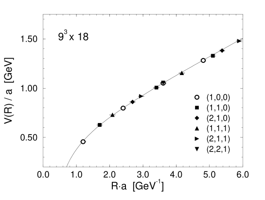
Figure 9: The same as Fig. 8 obtained on the $9{{}^{3}}{\times}18$ lattice.

Therefore, we perform two kinds of fits at $\beta=\beta_{c}(9^{3}\times 3)$: In the first fit, we fix the value of $\alpha$ to the average value 0.296 of those at the other two $\beta_{c}$’s which are constant within the errors. We set the fit range to be $R=2\;-\;2\sqrt{5}$ so that the physical $R$ range is consistent with the ranges at $\beta_{c}(12{{}^{3}}{\times}4)$ and $\beta_{c}(18{{}^{3}}{\times}6)$. As shown in Fig. 9, the fit well reproduces the data even at $R<R_{\rm min}$. In the other fit, we perform fit without fixing the value of $\alpha$, for the ranges $R_{\rm min}=\sqrt{2},\sqrt{3}$, and $2$ and $R_{\rm max}=2\sqrt{5}$. These values of $R_{\rm min}$ in physical units correspond to those at the other two $\beta_{c}$’s for which the stability of $\alpha$ is observed.

We take the results of the former fit with $\alpha$ fixed as the central values of $\sigma_{\rm lat}$ and $V_{0}$. The statistical errors are obtained by the jackknife method with bin size 1. We then take the upper bounds and lower bounds of $V_{0}$ and $\sigma_{\rm lat}$ obtained by the fits $\alpha$ unfixed, as systematic errors. The results of $V_{0}$ and $\sigma_{\rm lat}$ with the errors are given in Table 16. The potential data are shown in Fig. 9 together with its fit curve ($\alpha$ fixed to 0.296). The deviations from the fit are at most 2% and the average of them is about 0.5%, which indicates that the rotational invariance is well restored even at this small value of $\beta$.

We also perform a fit with $\alpha$ fixed to $\pi/12$ to find $\sigma_{\rm lat}=0.2607(16)$. The ratio $T_{c}/\sqrt{\sigma}$ using this result is consistent with our final result using the value in Table 16 within the errors.

4 Scaling properties

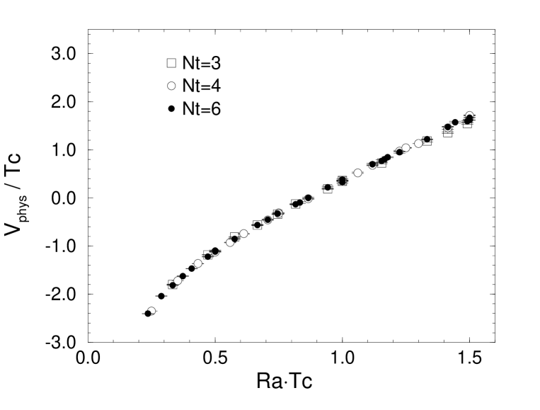
Figure 10: $V_{\rm phys}/{T_{c}}$ vs. $Ra{\cdot}T_{c}$. The constant term in the potential is fixed so that the potentials have the same value at $Ra{\cdot}T_{c}=1.0$.

In Fig. 10, the values of $V_{\rm phys}/T_{c}$ are shown as a function of $Ra\cdot T_{c}$, where $V_{\rm phys}=V/a$ is the potential in physical units. We note that the data on all the lattices are in excellent agreement in the whole $Ra\cdot T_{c}$ region. This implies scaling of our potential data in the range of $\beta$ values investigated. It might be emphasized again that the deviation of the data from the rotationally invariant fit is at most 2 % for the $N_{t}=3$ and 4 cases and 1 % for the $N_{t}=6$ case.

Using the results presented in the preceding section, we obtain the values of $T_{c}/\sqrt{\sigma}$ on the lattices with finite spatial volume $9^{3}$, $12^{3}$, and $18^{3}$, which equal to $(3/T_{c})^{3}\approx(2.2{\rm fm})^{3}$ in physical units:

$$T_{c}/\sqrt{\sigma}({\rm finite\ volume})=\left\{\begin{array}[]{ll}0.660(3)(^{+14}_{-10})&(N_{t}=3)\\ 0.647(5)&(N_{t}=4)\\ 0.651(6)&(N_{t}=6){{}_{.}}\end{array}\right.$$ (10)

The number in the first brackets is the statistical error and the second one for $N_{t}=3$ is the systematic error due to uncertainty of the fitting range.

In order to estimate the values of $T_{c}/\sqrt{\sigma}$ in the infinite volume limit, we first obtain finite size scaling relations [7, 8]

$$\beta_{c}(N_{t},N_{s}^{3})=\beta_{c}(N_{t},\infty)-{0.122(54)}\;{\cdot}\;{{N_{t}}^{3}}/{N_{s}^{3}}\;\;(N_{t}=3),$$ (11)

and

$$\beta_{c}(N_{t},N_{s}^{3})=\beta_{c}(N_{t},\infty)-{0.133(63)}\;{\cdot}\;{{N_{t}}^{3}}/{N_{s}^{3}}\;\;(N_{t}=4),$$ (12)

from the data of $\beta_{c}$ on the $N_{s}/N_{t}=3$, 4, and 5 lattices (see Fig. 11). We note that the slopes of $\beta_{c}(N_{t},N_{s}^{3})$ in $N_{t}^{3}/N_{s}^{3}$ in the two relations are independent of $N_{t}$ within the errors, as observed previously in the case of the standard one-plaquette action [8]. Therefore, we assume the relation (12) also for $N_{t}=6$. Then we have

$$\beta_{c}(N_{t},\infty)=\left\{\begin{array}[]{ll}2.1551(12)&(N_{t}=3)\\ 2.2879(11)&(N_{t}=4)\\ 2.5206(30)&(N_{t}=6){{}_{.}}\end{array}\right.$$ (13)

The values of the string tension at $\beta_{c}(N_{t},\infty)$ are estimated assuming an exponential scaling of $\sqrt{\sigma_{\rm lat}}$ in terms of $\beta$ [16]. We obtain

$$\sqrt{\sigma_{\rm lat}}=25.26(43)\;{\cdot}\;\exp\left[\;-1.828(7){\cdot}\beta\;\right],$$ (14)

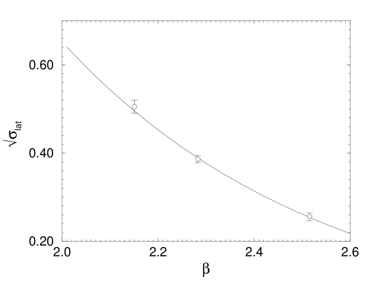
Figure 12: Square root of the string tension ${\sqrt{\sigma}_{\rm lat}}$ at $\beta_{c}$ on the finite volume lattices simulated together with its fitting curve.

by fitting the values of $\sigma_{\rm lat}$ at $\beta_{c}(9{{}^{3}}\times 3)$, $\beta_{c}(12{{}^{3}}\times 4)$, and $\beta_{c}(18{{}^{3}}\times 6)$ as shown in Fig. 12. This relation is used to compute the shifts in $\sigma_{\rm lat}$ from the values at $\beta_{c}(N_{t},N_{s}^{3})$ to those at $\beta_{c}(N_{t},\infty)$. The values of $\sigma_{\rm lat}(\beta_{c}(N_{t},\infty))$ are obtained by adding the shifts to those of $\sigma_{\rm lat}(\beta_{c}(N_{t},N_{s}^{3}))$ given in Tables 14 and 16:

$$\sigma_{\rm lat}(\beta_{c}(N_{t},\infty))=\left\{\begin{array}[]{ll}0.2516(26)(11)(^{+72}_{-110})&(N_{t}=3)\\ 0.1464(25)(6)&(N_{t}=4)\\ 0.0644(12)(7)&(N_{t}=6){{}_{.}}\end{array}\right.$$ (15)

The number in the first brackets is the statistical error, the second one is the error due to the error in the values of $\beta_{c}(N_{t},\infty)$, and the third one for $N_{t}=3$ is the systematic error due to uncertainty of the fitting range.

Finally, we obtain

$$T_{c}/\sqrt{\sigma}({\rm infinite\ volume})=\left\{\begin{array}[]{ll}0.665(3)(1)(^{+15}_{-10})&(N_{t}=3)\\ 0.653(6)(1)&(N_{t}=4)\\ 0.657(6)(4)&(N_{t}=6){{}_{.}}\end{array}\right.$$ (16)

The origins of the errors are the same as in Eq.(15). Our three values are consistent with a constant within the errors. A weighted average of the values given in Eq.(16) gives

$$T_{c}/\sqrt{\sigma}=0.656(4)$$ (17)

in the continuum limit.

Using the experimental value $\sigma=\sigma_{\rm lat}/a^{2}=(420\mbox{MeV})^{2}$, we obtain $a\approx 0.23$, 0.18, and 0.12 fm at $\beta_{c}$ for $N_{t}=3$, 4, and 6, respectively. Thus the scaling behavior for the ratio $T_{c}/\sqrt{\sigma}$ starts at least around $a\approx 0.23$fm with the RG improved gauge action. From Eq.(17) we also obtain $T_{c}\approx 276(2)\mbox{MeV}$.

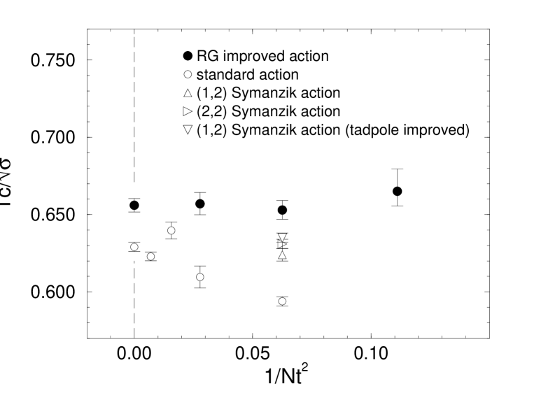
Figure 13: $T_{c}/{\sqrt{\sigma}}$ vs. $1/{{N_{t}}^{2}}$. All symbols represent the values in the infinite volume limit. The errors for our data in the cases of $N_{t}=4$ and 6 are statistical, while those for $N_{t}=3$ include the systematic error due to uncertainty of the fitting range.

Our results (16) are shown in Fig. 13 together with the results using other actions [4, 16]. Our result $T_{c}/\sqrt{\sigma}=0.656(4)$ in the continuum limit is slightly larger than the value with the standard action $0.629(3)$ [16]. We also compare our results with those derived from the torelon mass $\mu(L)$ which is calculated from Polyakov line correlators on a lattice of spatial size $L$. Defining $\sigma(L)=\mu(L)/L$, we extrapolate the values of $T_{c}/\sqrt{\sigma(L)}$ to the continuum limit. Then the value of $T_{c}/\sqrt{\sigma}$ is estimated assuming the relation $\sigma=\sigma(L)+\pi/(3L^{2})$ derived in a string model [17]. (We neglect the corrections due to the shift $\beta_{c}(V=\infty)-\beta_{c}(V=N_{s}^{3})$.) For a fixed point action [2], we obtain $T_{c}/\sqrt{\sigma}$ = 0.617(5) using the data for $N_{t}=2$, 3 and 4 with $N_{s}=2N_{t}$. The result is about 6% smaller than our result (17). For a tadpole-improved Symanzik action [3], we obtain $T_{c}/\sqrt{\sigma}$ = 0.649(5) using the data for $N_{t}=3$ and 4 with $N_{s}=2N_{t}$. The result is consistent with our result.

Numerical simulations are performed with Fujitsu VPP500/30 and HITAC H6080-FP12 at the University of Tsukuba. We thank Akira Ukawa for valuable discussions. This work is in part supported by the Grants-in-Aid of Ministry of Education, Science and Culture (Nos.07NP0401, 07640375 and 07640376) and the University of Tsukuba Project Research in 1996.

Table 1: Parameters of finite temperature simulations

lattice size	$\beta$	sweep	therm.
$9^{3}\times 3$	2.125	100000	30000
	2.145	100000	30000
	2.160	70000	30000
$12^{3}\times 3$	2.150	100000	50000
	2.155	100000	40000
$15^{3}\times 3$	2.150	180000	80000
$12^{3}\times 4$	2.250	12000	2000
	2.275	125000	40000
	2.300	10000	1500
$16^{3}\times 4$	2.283	220000	40000
	2.290	240000	40000
$20^{3}\times 4$	2.2875	270000	80000
$18^{3}\times 6$	2.5000	120000	15000
	2.5125	256000	50000
	2.5250	210000	60000
	2.5375	135000	5000

Table 2: Results obtained on the $9{{}^{3}}\times 3$ lattice.

	$\beta=2.125$	$\beta=2.145$	$\beta=2.160$
$1\times 1$ Wilson loop	0.575350(61)	0.58207(12)	0.58752(15)
$1\times 2$ Wilson loop	0.32181(11)	0.33120(22)	0.33917(28)
$2\times 2$ Wilson loop	0.10721(18)	0.11600(32)	0.12436(43)
Polyakov line	0.0675(23)	0.1055(40)	0.1575(52)
deconfinement fraction	0.448(23)	0.666(29)	0.895(29)

Table 3: Results obtained on the $12{{}^{3}}\times 3$ lattice.

	$\beta=2.150$	$\beta=2.155$
$1\times 1$ Wilson loop	0.58329(16)	0.58546(11)
$1\times 2$ Wilson loop	0.33277(31)	0.33607(20)
$2\times 2$ Wilson loop	0.11716(47)	0.12094(31)
Polyakov line	0.0972(74)	0.1300(38)
deconfinement fraction	0.691(53)	0.899(24)

Table 4: Results obtained on the $15{{}^{3}}\times 3$ lattice.

	$\beta=2.150$
$1\times 1$ Wilson loop	0.58321(17)
$1\times 2$ Wilson loop	0.33260(32)
$2\times 2$ Wilson loop	0.11688(48)
Polyakov line	0.0862(57)
deconfinement fraction	0.715(52)

Table 5: Results obtained on the $12{{}^{3}}\times 4$ lattice.

	$\beta=2.250$	$\beta=2.275$	$\beta=2.300$
$1\times 1$ Wilson loop	0.608085(91)	0.614037(60)	0.62007(28)
$1\times 2$ Wilson loop	0.36552(18)	0.37384(12)	0.38255(52)
$2\times 2$ Wilson loop	0.14448(25)	0.15257(19)	0.16175(76)
Polyakov line	0.0374(25)	0.0651(31)	0.1213(16)
deconfinement fraction	0.342(33)	0.640(23)	0.981(23)

Table 6: Results obtained on the $16{{}^{3}}\times 4$ lattice.

	$\beta=2.283$	$\beta=2.290$
$1\times 1$ Wilson loop	0.615677(33)	0.617594(35)
$1\times 2$ Wilson loop	0.376040(65)	0.378940(69)
$2\times 2$ Wilson loop	0.15451(10)	0.15781(11))
Polyakov line	0.0549(30)	0.0906(30)
deconfinement fraction	0.583(39)	0.853(27)

Table 7: Results obtained on the $20{{}^{3}}\times 4$ lattice.

	$\beta=2.2875$
$1\times 1$ Wilson loop	0.616941(56)
$1\times 2$ Wilson loop	0.37794(11)
$2\times 2$ Wilson loop	0.15663(19)
Polyakov line	0.0744(57)
deconfinement fraction	0.768(48)

Table 8: Results obtained on the $18{{}^{3}}\times 6$ lattice.

	$\beta=2.5000$	$\beta=2.5125$	$\beta=2.5250$	$\beta=2.5375$
$1\times 1$ Wilson loop	0.655687(59)	0.657691(11)	0.659676(11)	0.661649(12)
$1\times 2$ Wilson loop	0.431669(40)	0.434539(25)	0.437385(24)	0.440230(24)
$1\times 3$ Wilson loop	0.288927(53)	0.291912(33)	0.294884(33)	0.297874(32)
$2\times 2$ Wilson loop	0.208714(77)	0.211717(46)	0.214735(47)	0.217780(34)
$2\times 3$ Wilson loop	0.109884(87)	0.112330(53)	0.114813(54)	0.117350(55)
$3\times 3$ Wilson loop	0.049770(87)	0.051480(54)	0.053261(58)	0.055096(59)
Polyakov line	0.0328(32)	0.0409(21)	0.0559(22)	0.0691(21)
deconfinement fraction	0.555(51)	0.645(36)	0.861(31)	0.960(15)

Table 9: The value of $\beta{{}_{c}}$ and its jack knife error determined by the peak location of the susceptibility, and the deconfinement fraction $r$ at $\beta_{c}$, together with the bin size adopted.

	$\beta_{c}$	$r$	bin size
$9{{}^{3}}\times 3$	2.1508(12)	0.757(25)	1000
$12{{}^{3}}\times 3$	2.1528(9)	0.771(48)	3000
$15{{}^{3}}\times 3$	2.1546(11)	0.894(33)	8000
$12{{}^{3}}\times 4$	2.2827(16)	0.774(47)	3000
$16{{}^{3}}\times 4$	2.2863(10)	0.765(37)	6000
$20{{}^{3}}\times 4$	2.2865(9)	0.742(52)	10000
$18{{}^{3}}\times 6$	2.5157(7)	0.698(34)	3000

Table 10: Deconfinement fraction $r$ at $\beta{{}_{c}}$ determined from the susceptibility in the case of the standard one-plaquette action. Data of the Polyakov line are taken from a previous simulation by the QCDPAX Collaboration [8].

lattice	$\beta_{c}$	$r$
$12^{3}\times 24\times 4$	5.69149	0.790(12)
$24^{3}\times 36\times 4$	5.69245	0.732(46)
$20{{}^{3}}\times 6$	5.8924	0.805(26)
$24{{}^{3}}\times 6$	5.89292	0.786(27)
$36^{3}\times 48\times 6$	5.89379	0.739(40)

Table 11: Simulation parameters for the quark potential measurements.

lattice size	$\beta$	thermalization	# of conf.
$9^{3}\times 18$	2.1508	5000	400
$12^{3}\times 24$	2.2827	5000	200
$18^{3}\times 36$	2.5157	10000	100

Table 12: Potential $V(R)$ and overlap function $C(R)$ at $\beta_{c}(12{{}^{3}}{\times}4)$ obtained on the $12{{}^{3}}\times 24$ lattice. The optimum smearing step $N_{\rm opt}$ is also given.

$R$	unit of R	$V(R)$	$C(R)$	$N_{opt}$
1.000	(1,0,0)	0.47408(35)	0.9997(8)	10
1.414	(1,1,0)	0.63207(60)	0.9987(14)	10
1.732	(1,1,1)	0.72136(89)	0.9955(23)	10
2.000	(1,0,0)	0.7811(12)	0.9916(31)	12
2.236	(2,1,0)	0.8304(11)	0.9880(25)	10
2.449	(2,1,1)	0.8759(12)	0.9977(29)	8
2.828	(1,1,0)	0.9472(17)	0.9990(43)	8
3.000	(1,0,0)	0.9843(27)	0.9857(72)	10
3.000	(2,2,1)	0.9806(19)	0.9799(48)	8
3.464	(1,1,1)	1.0574(32)	0.9739(86)	8
4.000	(1,0,0)	1.1507(15)	0.9779(41)	8
4.243	(1,1,0)	1.1926(45)	0.982(12)	8
4.472	(2,1,0)	1.2317(41)	0.976(11)	8
4.899	(2,1,1)	1.3053(55)	0.971(15)	8
5.000	(1,0,0)	1.3222(22)	0.9881(63)	8
5.196	(1,1,1)	1.34430(55)	0.9925(57)	6
5.657	(1,1,0)	1.426(11)	0.982(29)	8
6.000	(1,0,0)	1.479(19)	0.978(53)	8
6.000	(2,2,1)	1.49012(78)	0.9966(66)	6

Table 13: The same as Table 12 at $\beta_{c}(18{{}^{3}}{\times}6)$ obtained on the $18{{}^{3}}\times 36$ lattice.

$R$	unit of R	$V(R)$	$C(R)$	$N_{opt}$
1.000	(1,0,0)	0.39187(22)	1.0059(7)	40
1.414	(1,1,0)	0.50809(29)	1.0065(10)	40
1.732	(1,1,1)	0.56917(44)	1.0059(17)	40
2.000	(1,0,0)	0.60693(62)	1.0042(21)	40
2.236	(2,1,0)	0.63812(56)	0.9991(19)	36
2.449	(2,1,1)	0.66409(68)	0.9991(21)	30
2.828	(1,1,0)	0.70597(77)	0.9964(25)	28
3.000	(1,0,0)	0.7270(12)	0.9983(40)	30
3.000	(2,2,1)	0.72320(82)	0.9986(27)	24
3.464	(1,1,1)	0.7671(14)	0.9970(49)	22
4.000	(1,0,0)	0.8151(18)	0.9985(67)	20
4.243	(1,1,0)	0.8340(18)	0.9915(58)	20
4.472	(2,1,0)	0.8548(17)	0.9933(56)	20
4.899	(2,1,1)	0.8872(19)	0.9914(65)	18
5.000	(1,0,0)	0.8929(31)	1.000(11)	16
5.196	(1,1,1)	0.9089(23)	1.0000(90)	16
5.657	(1,1,0)	0.9462(28)	0.9894(97)	18
6.000	(1,0,0)	0.9644(39)	0.993(15)	14
6.000	(2,2,1)	0.9721(29)	0.992(10)	16
6.708	(2,1,0)	1.0254(34)	0.982(11)	18
6.928	(1,1,1)	1.0374(43)	0.984(15)	16
7.000	(1,0,0)	1.04334(53)	0.9905(64)	16
7.071	(1,1,0)	1.0501(18)	0.9983(84)	16
7.348	(2,1,1)	1.0674(41)	0.995(14)	14
8.000	(1,0,0)	1.11216(68)	0.9953(78)	14
8.485	(1,1,0)	1.15463(52)	0.9998(84)	16
8.660	(1,1,1)	1.1714(32)	0.988(14)	18
8.944	(2,1,0)	1.1743(22)	0.9870(78)	12
9.000	(1,0,0)	1.17869(54)	0.9794(86)	14
9.000	(2,2,1)	1.18690(47)	0.9975(78)	12

Table 14: Results of $V_{0}$, $\alpha$, and $\sigma_{\rm lat}$ at $\beta_{c}(12{{}^{3}}{\times}4)$ and $\beta_{c}(18{{}^{3}}{\times}6)$ obtained on the $12{{}^{3}}{\times}24$ and $18{{}^{3}}{\times}36$ lattices, respectively.

$\beta$	$V_{0}$	$\alpha$	$\sigma_{\rm lat}$
$\beta_{c}(12{{}^{3}}\times 4)$	0.630(20)	0.295(14)	0.1493(25)
$\beta_{c}(18{{}^{3}}\times 6)$	0.627(18)	0.297(19)	0.0655(12)

Table 15: The same as Table 12 at $\beta_{c}(9^{3}\times 3)$ obtained on the $9{{}^{3}}\times 18$ lattice.

$R$	unit of R	$V(R)$	$C(R)$	$N_{opt}$
1.000	(1,0,0)	0.54892(35)	0.9982(5)	4
1.414	(1,1,0)	0.75390(63)	0.9984(10)	4
1.732	(1,1,1)	0.87752(99)	0.9942(16)	4
2.000	(1,0,0)	0.9601(13)	0.9981(22)	5
2.236	(2,1,0)	1.0349(13)	0.9965(21)	4
2.449	(2,1,1)	1.1049(15)	0.9963(25)	2
2.828	(1,1,0)	1.2101(22)	0.9945(39)	4
3.000	(1,0,0)	1.2640(31)	0.9836(55)	5
3.000	(2,2,1)	1.2685(23)	0.9591(39)	3
3.464	(1,1,1)	1.3890(41)	0.9736(73)	4
4.000	(1,0,0)	1.5420(18)	0.9750(34)	5
4.243	(1,1,0)	1.6001(60)	0.987(12)	4
4.472	(2,1,0)	1.6634(62)	0.978(11)	4
4.899	(2,1,1)	1.7785(53)	0.973(13)	3

Table 16: Results of $V_{0}$ and $\sigma_{\rm lat}$ at $\beta_{c}(9^{3}\times 3)$ obtained on the $9^{3}\times 18$ lattice. The numbers in the first brackets are statistical errors and the second are systematic errors due to uncertainty of the fitting range.

$V_{0}$	$\sigma_{\rm lat}$
0.598(60)(${}^{+57}_{-48}$)	0.2554(26)(${}^{+72}_{-110}$)

Figure 6: $T$ dependence of $m_{\rm eff}=\mbox{log}\left[W(R,T)/W(R,T+1)\right]$ without (a) and with (b) smearing on the $12{{}^{3}}\times 24$ lattice. The results shown in (b) are obtained with the optimum smearing step explained in the text.

Figure 11: Finite size scaling of $\beta_{c}$ on $N_{t}=3$ and $4$ lattices. The solid lines are the results of a linear fit and the dashed lines indicate the location of the infinite volume limit.

References

- [1] G. Cella, G. Curci, A. Vicere, and B. Vigna, Phys. Lett. B333 (1994) 457.
- [2] T. DeGrand, A. Hasenfratz, P. Hasenfratz, and F. Niedermayer, Nucl. Phys. B454 (1995) 615.
- [3] D.W. Bliss, K. Hornbostel, and G.P. Lepage, Southern Methodist Univ. report SMUHEP 96-05 (hep-lat/9605041).
- [4] F. Karsch, B. Beinlich, J. Engels, R. Joswig, E. Laermann, A. Peikert, and B. Petersson, Univ. Bielefeld report BI-TP-96-34 (hep-lat/9608047).
- [5] For a recent review, see A. Ukawa, review talk presented at Lattice 96, to be published in the proceedings.
- [6] Y. Iwasaki, Nucl. Phys. B258 (1985) 141; Univ. of Tsukuba report UTHEP-118 (1983), unpublished.
- [7] M. Fukugita, M. Okawa and A. Ukawa, Nucl. Phys. B337(1990)181.
- [8] QCDPAX Collaboration: Y. Iwasaki et al., Phys. Rev. D46 (1992) 4657.
- [9] I.R. McDonald and K. Singer, Discuss. Faraday Soc. 43 (1967) 40; A.M. Ferrenberg and R.H. Swendsen, Phys. Rev. Lett. 61 (1988) 2635; 63 (1989) 1195.
- [10] S. A. Gottlieb, J. Kuti, D. Toussaint, A.D. Kennedy, S. Meyer, B. J. Pendleton and R. L. Sugar, Phys. Rev. Lett. 55 (1985) 1958.
- [11] N. Christ and A. Terrano, Phys. Rev. Lett. 56 (1986) 111.
- [12] D. Toussaint, in the proceedings of Lattice ’86, H. Satz et al. eds., Plenum, (1987) 399.
- [13] C. Borgs, R. Kotecký, and S. Miracle-Solé, J. Stat. Phys. 62 (1991) 529.
- [14] G.S. Bali and K. Schilling, Phys. Rev. D46 (1992) 2636.
- [15] M. Lüscher, K. Symanzik, and P. Weisz, Nucl. Phys. B173 (1980) 365.
- [16] G. Boyd, J. Engels, F. Karsch, E. Laermann, C. Legeland, M. Lütgemeier, and B. Petersson, Univ. Bielefeld report BI-TP-96-04 (hep-lat/9602007).
- [17] Ph. de Forcrand, G. Schierholz, H. Schneider, and M. Taper, Phys. Lett. B160 (1985) 137.