Multi-Grid Monte Carlo via $XY$ Embedding
II. Two-Dimensional $SU(3)$ Principal Chiral Model

Abstract

We carry out a high-precision simulation of the two-dimensional $SU(3)$ principal chiral model at correlation lengths $\xi$ up to $\sim\!4\times 10^{5}$, using a multi-grid Monte Carlo (MGMC) algorithm and approximately one year of Cray C-90 CPU time. We extrapolate the finite-volume Monte Carlo data to infinite volume using finite-size-scaling theory, and we discuss carefully the systematic and statistical errors in this extrapolation. We then compare the extrapolated data to the renormalization-group predictions. The deviation from asymptotic scaling, which is $\approx 12\%$ at $\xi\sim 25$, decreases to $\approx 2\%$ at $\xi\sim 4\times 10^{5}$. We also analyze the dynamic critical behavior of the MGMC algorithm using lattices up to $256\times 256$, finding the dynamic critical exponent $z_{int,{\cal M}^{2}}\approx 0.45\pm 0.02$ (subjective 68% confidence interval). Thus, for this asymptotically free model, critical slowing-down is greatly reduced compared to local algorithms, but not completely eliminated.

1 Introduction

This paper has two distinct objectives: first, to study the dynamic critical behavior of the multi-grid Monte Carlo (MGMC) algorithm for the two-dimensional $SU(3)$ principal chiral model; and second, to apply this algorithm to obtain a high-precision test of asymptotic scaling for this model. We discuss these two objectives in separate subsections.

1.1 Multi-Grid Monte Carlo

By now it is widely recognized [1, 2, 3, 4] that better simulation algorithms, with strongly reduced critical slowing-down, are needed for high-precision Monte Carlo studies of statistical-mechanical systems near critical points and of quantum field theories (such as QCD) near the continuum limit. One promising class of such algorithms is multi-grid Monte Carlo (MGMC) [5, 6, 7, 8, 9, 10, 11, 12, 13, 14, 15, 16, 17, 18, 19, 20, 21, 22, 23, 24, 25, 26, 27, 28]: this is a collective-mode approach that introduces block updates (of fixed shape but variable amplitude) on all length scales. The basic ingredients of the method are:

1) Interpolation operator: This is a rule specifying the shape of the block update. The interpolations most commonly used are piecewise-constant (square-wave updates) and piecewise-linear (pyramidal-wave updates).

2) Cycle control parameter $\gamma$: This is an integer number that determines the way in which the different block sizes are visited. In general, blocks of linear size $2^{l}$ are updated $\gamma^{l}$ times per iteration. Thus, in the W-cycle ($\gamma=2$) more emphasis is placed on large length scales than in the V-cycle ($\gamma=1$).

3) Basic (smoothing) iteration: This is the local Monte Carlo update that is performed on each level. Typically one chooses to use heat-bath updating if the distribution can be sampled in some simple way, and Metropolis updating otherwise.

4) Implementation: The computations can be implemented either in the recursive multi-grid style using explicit coarse-grid fields [29, 30, 5, 6, 7, 8, 9, 10, 11], or in the unigrid style using block updates acting directly on the fine-grid fields [31, 14, 15, 16, 17, 18]. We use here the recursive multi-grid approach, in which the computational labor per iteration for a $d$-dimensional system of linear size $L$ is

$$\hbox{Work(MG)}\;\sim\;\cases{L^{d}&for $\gamma<2^{d}$\cr\vskip 2.84526pt\cr L^{d}\,\log L&for $\gamma=2^{d}$\cr\vskip 2.84526pt\cr L^{\log_{2}\gamma}&for $\gamma>2^{d}$\cr}$$ (1.1)

The efficiency of the MGMC method can be analyzed rigorously in the case of the Gaussian (free-field) model, for which it can be proven [5, 6, 32] that critical slowing-down is completely eliminated. That is, the autocorrelation time $\tau$ is bounded as the correlation length $\xi$ and the lattice size $L$ tend to infinity, so that the dynamic critical exponent $z$ is zero.

One is therefore motivated to apply MGMC to “nearly Gaussian” systems, such as asymptotically free nonlinear $\sigma$-models; one might hope that critical slowing-down would likewise be completely eliminated (possibly modulo a logarithm) or at least greatly reduced compared to the $z\approx 2$ of local algorithms. However, previous numerical study of MGMC in the two-dimensional $N$-vector models with $N=3,4,8$ [8, 11] has shown, to our initial surprise, that the dynamic critical exponent is not zero. Nevertheless, it is quite small ($z\approx 0.50$–0.70), so these algorithms work reasonably well. In view of these results for the $N$-vector models, we want to investigate the performance of MGMC in other asymptotically free $\sigma$-models, such as the two-dimensional $SU(N)$ principal chiral models.

Of course, for two-dimensional $N$-vector models, Wolff’s cluster algorithm [33] apparently succeeds in eliminating the critical slowing-down [33, 34, 35, 36], so there is no point in using MGMC in this case. But there are strong reasons to believe [36] that Wolff-type embedding algorithms will not achieve $z\ll 2$ for other $\sigma$-models, except perhaps the $RP^{N-1}$ models. In particular, for $\sigma$-models taking values in the group $SU(N)$ with $N\geq 3$, MGMC is the only known collective-mode algorithm (except perhaps Fourier acceleration) that has a chance of achieving $z\ll 2$.

A major drawback of our group’s standard MGMC [5, 6, 7, 8, 9] is that its implementation is cumbersome and model-dependent, in the sense that the program (and in particular the heat-bath subroutine) has to be drastically rewritten for each distinct model. With this problem in mind, we have recently developed [10, 11] a new implementation of MGMC that can be used conveniently for a large class of $\sigma$-models with very little modification of the program. The idea is to embed angular variables $\{\theta_{x}\}$ into the given $\sigma$-model, and then update the resulting induced $XY$ model by our standard (piecewise-constant, W-cycle, heat-bath, recursive) MGMC method.

Consider, therefore, the $SU(N)$ principal chiral model: the original variables $U_{x}$ of this model are $SU(N)$ matrices living on the lattice sites $x$, and the original Hamiltonian is

$${\cal H}\;=\;-\beta\sum_{\langle xx^{\prime}\rangle}\mathop{\rm Re}\nolimits\mathop{\rm tr}\nolimits(U_{x}^{\dagger}\,U_{x^{\prime}})\;.$$ (1.2)

The global symmetry group is $SU(N)_{{\hbox{\scriptsize\it left}}}\times SU(N)_{{\hbox{\scriptsize\it right}}}$. The idea behind $XY$ embedding is to choose randomly a $U(1)$ subgroup $H\subset SU(N)_{{\hbox{\scriptsize\it left}}}\times SU(N)_{{\hbox{\scriptsize\it right}}}$, and to apply a “rotation” $\theta_{x}$ in this subgroup to the original spin variable $U_{x}\in SU(N)$. Thus, the angular variables $\theta_{x}$ are updates to the original variables $U_{x}$. Here we choose to exploit only the left-multiplication subgroup. More precisely, we define the updated variable $U_{x}^{new}$ by

$$U_{x}^{new}\;=\;e^{i\theta_{x}RTR^{-1}}U_{x}^{old}\;=\;Re^{i\theta_{x}T}R^{-1}U_{x}^{old}\;,$$ (1.3)

where $R$ is a random element of $SU(N)$, and $T$ is a fixed nonzero element (to be specified later) of the Lie algebra ${\hbox{\german su}(N)}$ (i.e. a traceless Hermitian matrix). The embedded $XY$ model consisting of the spins $\{\theta_{x}\}$ is then simulated using the induced Hamiltonian

$${\cal H}_{embed}(\{\theta_{x}\})\;=\;{\cal H}(\{U_{x}^{new}\})\;,$$ (1.4)

with initial condition $\theta_{x}=0$ (i.e. $U_{x}^{new}=U_{x}^{old}$) for all $x$. At each iteration of the algorithm, a new random matrix $R$ is chosen.

In general the induced $XY$ Hamiltonian (1.4) can be extremely complicated (and thus impractical to simulate by true recursive MGMC). However, if the original Hamiltonian ${\cal H}$ is sufficiently “nice” and one makes a clever choice of the generator $T$, then in some cases the induced $XY$ Hamiltonian can be reasonably simple. In particular, if we choose $T$ to have all its eigenvalues in the set $\{-1,0,1\}$, it follows that

$$e^{i\theta T}\;=\;T^{2}\,\cos\theta\,+\,iT\,\sin\theta\,+\,(I\,-\,T^{2})\;,$$ (1.5)

where $I$ is the identity matrix. Then the induced Hamiltonian is of the simple form

$${\cal H}_{embed}\;=\;-\sum_{\langle xx^{\prime}\rangle}\left[\alpha_{xx^{\prime}}\,\cos(\theta_{x}\,-\,\theta_{x^{\prime}})\,+\,\beta_{xx^{\prime}}\,\sin(\theta_{x}\,-\,\theta_{x^{\prime}})\right]\,+\,{\rm const}\;,$$ (1.6)

where the induced couplings $\{\alpha_{xx^{\prime}},\beta_{xx^{\prime}}\}$ depend on the current configuration $\{U_{x}^{old}\}$ of the original model:

$$\alpha_{xx^{\prime}}&=\beta\,\mathop{\rm Re}\nolimits\mathop{\rm tr}\nolimits(U_{x}^{old\dagger}RT^{2}R^{-1}U^{old}_{x^{\prime}})\\ \beta_{xx^{\prime}}=\beta\,\mathop{\rm Re}\nolimits\mathop{\rm tr}\nolimits(U_{x}^{old\dagger}R(-iT)R^{-1}U^{old}_{x^{\prime}})\;=\;\beta\,\mathop{\rm Im}\nolimits\mathop{\rm tr}\nolimits(U_{x}^{old\dagger}RTR^{-1}U^{old}_{x^{\prime}})$$ (1.7)

Such a “generalized $XY$ Hamiltonian” is easily simulated by MGMC; indeed, the coarse-grid Hamiltonians in $XY$-model MGMC are inevitably of the form (1.6), even when the fine-grid Hamiltonian is the standard $XY$ model $\alpha_{xx^{\prime}}\equiv\alpha\geq 0$, $\beta_{xx^{\prime}}\equiv 0$ [6, 7]. So one may just as easily start from (1.6) already on the finest grid.

Clearly $T$ must have $k$ eigenvalues $+1$, $k$ eigenvalues $-1$, and $N-2k$ eigenvalues 0, where $1\leq k\leq\lfloor N/2\rfloor$. Here we shall choose $k=1$; without loss of generality we can take

$$T\;=\;\left(\begin{array}[]{cccc}1&0&0&\\ 0&-1&0&\cdots\\ 0&0&0&\\ &\vdots&&\ddots\end{array}\right)\;.$$ (1.8)

With the explicit choice (1.8) for $T$, the couplings are

$$\alpha_{xx^{\prime}}&=\beta\,\left[\mathop{\rm Re}\nolimits(R^{-1}\,U^{old}_{x^{\prime}}\,U_{x}^{old\dagger}\,R)_{11}\,+\,\mathop{\rm Re}\nolimits(R^{-1}\,U^{old}_{x^{\prime}}\,U_{x}^{old\dagger}\,R)_{22}\right]\\ \beta_{xx^{\prime}}=\beta\,\left[\mathop{\rm Im}\nolimits(R^{-1}\,U^{old}_{x^{\prime}}\,U_{x}^{old\dagger}\,R)_{11}\,-\,\mathop{\rm Im}\nolimits(R^{-1}\,U^{old}_{x^{\prime}}\,U_{x}^{old\dagger}\,R)_{22}\right]\;.$$ (1.9)

Let us remark that the Hamiltonian (1.6)/(1.7) is not only non-ferromagnetic, but is in fact typically frustrated [11]. However, this frustration is weak when $\beta\gg 1$.

1.2 Asymptotic Scaling

A key tenet of modern elementary-particle physics is the asymptotic freedom of four-dimensional nonabelian gauge theories [37, 38]. However, the nonperturbative validity of asymptotic freedom has been questioned [39, 40, 41, 42]; and numerical studies of lattice gauge theory have thus far failed to detect asymptotic scaling in the bare coupling [43, 44, 45, 46]. It is therefore useful to explore asymptotic scaling in a model easier to simulate numerically than four-dimensional gauge theories, but still theoretically interesting. A good candidate is the two-dimensional $SU(N)$ principal chiral model (1.2), which possesses the property of perturbative asymptotic freedom [47, 48, 49] along with other interesting characteristics.

Let us recall the logic underlying the conventional wisdom on asymptotic freedom: Renormalization-group (RG) calculations in weak-coupling (large-$\beta$) perturbation theory show that for two-dimensional $\sigma$-models taking values in a curved compact Riemannian manifold $M$, the RG flow at large $\beta\equiv 1/g^{2}$ is toward smaller $\beta$ [47, 48, 49, 55, 56, 57, 58]. It is therefore natural to conjecture that this flow continues to the $\beta=0$ fixed point, without encountering any other fixed point(s). If this is indeed the case, then it follows that the theory has exponential decay of correlations for all $\beta<\infty$; and the RG then gives precise predictions for the scaling behavior of the correlation length $\xi$ and the susceptibility $\chi$ as $\beta\to\infty$. Moreover, for certain $\sigma$-models it is possible to calculate, modulo some plausible hypotheses, the nonperturbative coefficient in the asymptotic formula for the correlation length [59, 60, 61, 62, 63, 64]. It should be emphasized, however, that all these results depend on a conjecture which transcends perturbation theory and which has thus far been neither proven nor disproven. This is why we want to test the nonperturbative validity of asymptotic freedom, using numerical simulations.

Let us clarify our use of the words “scaling” and “asymptotic scaling”. Consider a sequence $\{{\cal H}_{n}\}_{n=1}^{\infty}$ of lattice theories with correlation lengths $\xi_{n}$ tending to infinity. We say that this sequence exhibits scaling if, after rescaling lengths by $\xi_{n}$ and rescaling the spins by appropriate values $\zeta_{n}$, all the correlation functions $\langle\;\cdots\;\rangle_{{\cal H}_{n}}$ converge to some continuum-limit values. Equivalently, the sequence exhibits scaling if all dimensionless ratios of long-distance observables tend to constants. More loosely, we say that a finite sequence of theories $\{{\cal H}_{n}\}_{n=1}^{N}$ exhibits scaling to within some given degree of accuracy if all dimensionless ratios of long-distance observables are constant within the given degree of accuracy. (This latter notion is often used in Monte Carlo work, expressed by some phrase like “we are in the scaling region” or “we are near the continuum limit”.) Note that the parameters in ${\cal H}_{n}$ (such as $\beta$) play no role in the concept of scaling.

Now consider a sequence $\{{\cal H}_{n}\}_{n=1}^{\infty}$ of lattice theories with correlation lengths $\xi_{n}$ tending to infinity, for which there exists a theoretical prediction for the asymptotic behavior of long-distance observables as a function of the parameters in ${\cal H}_{n}$ (or as a function of short-distance observables like the energy). [The example of interest is of course an asymptotically free theory in the limit $\beta\to\infty$, where the renormalization group predicts ${\cal O}(\beta)=Ce^{a\beta}\beta^{b}(1+a_{1}/\beta+a_{2}/\beta^{2}+\ldots)$ for each long-distance observable ${\cal O}$, with $a,b,a_{1},a_{2},\ldots$ computable in perturbation theory but $C$ usually unknown.] We say that the given sequence exhibits asymptotic scaling if the theoretical predictions for the leading-order asymptotic behavior are valid. [In the asymptotically-free case this means that ${\cal O}(\beta_{n})/(e^{a\beta_{n}}\beta_{n}^{b})$ tends to a constant as $n\to\infty$.] More loosely, we say that a finite sequence of theories $\{{\cal H}_{n}\}_{n=1}^{N}$ exhibits asymptotic scaling to within some given degree of accuracy if the theoretical predictions for the leading-order asymptotic behavior are valid to within the given degree of accuracy. [In the asymptotically-free case this means that ${\cal O}(\beta_{n})/(e^{a\beta_{n}}\beta_{n}^{b})$ is constant to within the given degree of accuracy.]

Clearly, asymptotic scaling implies scaling (if the observables behave correctly as a function of $\beta$, then their dimensionless ratios necessarily converge), but not conversely. Note also that even if asymptotic scaling does hold along the given path in parameter space, it may be necessary to go to much larger correlation lengths to observe asymptotic scaling to some reasonable degree of accuracy than to observe scaling to the same degree of accuracy.

In the renormalization-group language, deviations from scaling are caused by irrelevant operators (so that the RG flow does not lie exactly on the unstable manifold), while deviations from asymptotic scaling arise also from higher-order corrections to the flow on the unstable manifold. In an asymptotically free theory, deviations from scaling are nonperturbative effects (suppressed by powers of $\xi$ and hence exponentially small in $\beta$), while deviations from asymptotic scaling are perturbative effects (a power series in $1/\beta\sim 1/\log\xi$, with coefficients that are computable in lattice perturbation theory). Therefore, scaling may be expected to set in at a rather modest correlation length (e.g. $\xi\sim 10$ or even smaller), because the corrections to scaling fall off like inverse powers of $\xi$. On the other hand, asymptotic scaling is much more elusive, because the corrections fall off like inverse powers of the logarithm of $\xi$: depending on the magnitude of the perturbative coefficients (including unknown high-order ones), asymptotic scaling could set in at correlation lengths as small as $\sim 10$ or could require correlation lengths as large as $\sim 10^{30}$.

Consequently it is not a surprise that numerical studies of lattice gauge theory have thus far failed to detect asymptotic scaling in the bare coupling. Even in the simpler case of two-dimensional nonlinear $\sigma$-models, numerical simulations at correlation lengths $\xi\sim 10$–100 have often shown discrepancies of order 10–50% from asymptotic scaling. In the $SU(3)$ chiral model, previous Monte Carlo studies [65, 17, 66, 67] up to $\xi\approx 35$ have found that the ratio $\xi(\beta)/[e^{a\beta}\beta^{b}(1+a_{1}/\beta)]$ is not approximately constant, nor does its value agree with the predicted nonperturbative coefficient [62]; on both points the discrepancy is of order 10–20%.

These studies seem to show empirically that to observe asymptotic scaling in the bare coupling in the $SU(3)$ chiral model, the numerical simulations will need to reach correlation lengths $\xi\gg 35$ (how large is not so clear). Unfortunately, it is at present unfeasible to simulate lattices of linear size $L$ bigger than $\sim 1000$; so, if we want to do a direct “infinite-volume” simulation, which requires $L/\xi\mathrel{\hbox to0.0pt{\lower 3.0pt\hbox{$\mathchar 536\relax$}\hss}\raise 2.0pt\hbox{$\mathchar 318\relax$}}6$–8 to avoid significant finite-size effects, we cannot hope to reach correlation lengths beyond about 150. To circumvent this problem, we shall resign ourselves to using lattices that are far from being “infinite”, and we shall attempt to understand the finite-size effects in such detail that we can correct for them. We do this by applying an extremely powerful method [68, 69] for the extrapolation of finite-size data to the infinite-volume limit, due originally to Lüscher, Weisz and Wolff [70] (see also Kim [71, 72, 73, 74, 75]), based on finite-size-scaling theory. Using only lattices $L\leq 256$, we are able to obtain the infinite-volume correlation length $\xi_{\infty}$ to an accuracy of order 0.5% (resp. 0.9%, 1.1%, 1.3%, 1.5%) when $\xi_{\infty}\approx 10^{2}$ (resp. $10^{3}$, $10^{4}$, $10^{5}$, $4\times 10^{5}$). We realize that this sounds crazy at first, but we hope to convince the reader that we do in fact have reliable control over all systematic and statistical errors (see Section 5 for details).

Finally, let us remark that other studies have used different approaches to observe either scaling or asymptotic scaling at smaller correlation lengths. Thus, the various “improved actions” (Symanzik [82, 83, 84, 85], Hasenfratz–Niedermayer [86, 87], etc.) are aimed at reaching scaling at the smallest possible correlation length. If they have any effect on asymptotic scaling, it is by coincidence rather than by design. On the other hand, the various “improved expansion parameters” are aimed at reaching asymptotic scaling at the smallest possible correlation length, by redefining slightly the meaning of “asymptotic scaling” (using the energy as the parameter in place of $\beta$).

In the model treated here, scaling is reached (to within about one percent) already at a correlation length of a few lattice spacings [67]. Since we are able to go to much larger correlation lengths than this, scaling is no problem at all for us; we thus have no need of “improved actions”. On the other hand, asymptotic scaling is much more elusive, and we are therefore very interested in trying out the proposed “improved expansion parameters”. But we have some reticence about the conceptual and theoretical basis underlying this approach (see Section 3.3).

1.3 Plan of this Paper

The plan of this paper is as follows: In Section 2 we set the notation. In Section 3 we summarize the perturbative predictions for the two-dimensional $SU(N)$ principal chiral models. In Section 4 we present our raw data, which are based on approximately one year of Cray C-90 CPU time. In Section 5 we carry out a detailed analysis of our static data, making systematic use of the finite-size-scaling extrapolation method, and we compare the extrapolated values with the perturbative predictions. In Section 6 we analyze our dynamic data using conventional finite-size-scaling plots to extract the dynamic critical exponents $z_{int,{\cal M}_{F}^{2}}$ and $z_{int,{\cal M}_{A}^{2}}$. In Appendices A and B we present some perturbative computations.

Parts of this work have appeared previously in brief preliminary reports [10, 12].

2 Notations and Preliminaries

2.1 Observables to be Measured

We wish to study various correlation functions of the fundamental-representation field $U_{x}$ and the adjoint-representation field $V_{x}$ defined by

$$(V_{x})^{\alpha\,\cdot\,\,\cdot\,\delta}_{\,\cdot\,\beta\gamma\,\cdot\,}\;\equiv\;(U_{x})^{\alpha}_{\,\cdot\,\gamma}(\overline{U_{x}})^{\,\cdot\,\delta}_{\beta}\,-\,{1\over N}\,\delta^{\alpha}_{\beta}\delta^{\delta}_{\gamma}\;.$$ (2.1)

Note the relation between the traces in the fundamental and the adjoint representations,

$$\mathop{\rm tr}\nolimits_{A}U\,\equiv\,\mathop{\rm tr}\nolimits V\,\equiv\,(V_{x})^{\alpha\,\cdot\,\,\cdot\,\beta}_{\,\cdot\,\beta\alpha\,\cdot\,}\;=\;|\mathop{\rm tr}\nolimits(U)|^{2}-1\;,$$ (2.2)

which follows immediately from (2.1). We thus define the fundamental and adjoint 2-point correlation functions

$$G_{F}(x-y)&=\langle\mathop{\rm tr}\nolimits(U_{x}^{\dagger}\,U_{y})\rangle\\ G_{A}(x-y)=\langle\mathop{\rm tr}\nolimits_{A}(U_{x}^{\dagger}\,U_{y})\rangle\;=\;\langle|\mathop{\rm tr}\nolimits(U_{x}^{\dagger}\,U_{y})|^{2}\rangle-1\;.$$ (2.3)

All our numerical work will be done on an $L\times L$ lattice with periodic boundary conditions. We are interested in the following quantities:

• The fundamental and adjoint energies

  $$E_{F}&={1\over N}\,\langle\mathop{\rm tr}\nolimits(U_{{\bf e}}^{\dagger}\,U_{0})\rangle\;=\;{1\over N}\,G_{F}({\bf e})\\ E_{A}={1\over N^{2}-1}\,(\langle|\mathop{\rm tr}\nolimits(U_{{\bf e}}^{\dagger}\,U_{0})|^{2}\rangle\,-\,1)\;=\;{1\over N^{2}-1}\,G_{A}({\bf e})$$ (2.4)

  where ${\bf e}$ stands for any nearest neighbor of the origin.

• The fundamental, adjoint and mixed specific heats

  $$C_{FF}&={d\over N}\sum\limits_{\langle yz\rangle}\langle\mathop{\rm Re}\nolimits\,\mathop{\rm tr}\nolimits(U^{\dagger}_{\bf e}\,U_{0})\,;\,\mathop{\rm Re}\nolimits\,\mathop{\rm tr}\nolimits(U^{\dagger}_{y}\,U_{z})\rangle\;=\;d{\partial E_{F}\over\partial\beta}\\ C_{AA}={d\over N^{2}-1}\sum\limits_{\langle yz\rangle}\langle|\mathop{\rm tr}\nolimits(U^{\dagger}_{\bf e}\,U_{0})|^{2}\,;\,|\mathop{\rm tr}\nolimits(U^{\dagger}_{y}\,U_{z})|^{2}\rangle\\ C_{FA}={d\over\sqrt{N^{2}-N}}\sum\limits_{\langle yz\rangle}\langle|\mathop{\rm tr}\nolimits(U^{\dagger}_{\bf e}\,U_{0})|^{2}\,;\,\mathop{\rm Re}\nolimits\,\mathop{\rm tr}\nolimits(U^{\dagger}_{y}\,U_{z})\rangle$$ (2.5)

  where ${\bf e}$ stands for any nearest neighbor of the origin, $d$ is the spatial dimension (in this paper $d=2$), and $\langle A;B\rangle\equiv\langle AB\rangle-\langle A\rangle\langle B\rangle$.

• The fundamental and adjoint magnetic susceptibilities

  $$\chi_{\#} = \sum\limits_{x}G_{\#}(x)\;,$$ (2.6)

  where $\#$ stands for $F$ or $A$.

• The fundamental and adjoint correlation functions at the smallest nonzero momentum:

  $$F_{\#} = \sum\limits_{x}e^{ip_{0}\cdot x}\,G_{\#}(x)\;,$$ (2.7)

  where $p_{0}=(\pm 2\pi/L,0)\hbox{ or }(0,\pm 2\pi/L)$.

• The fundamental and adjoint second-moment correlation lengths

  $$\xi^{(2nd)}_{\#} = {(\chi_{\#}/F_{\#}\,-\,1)^{1/2}\over 2\sin(\pi/L)}\;.$$ (2.8)

  In the infinite-volume limit this becomes

  $$\xi^{(2nd)}_{\#}\;=\;\left({1\over 2d}\,{\displaystyle\sum\limits_{x}|x|^{2}G_{\#}(x)\over\displaystyle\sum\limits_{x}G_{\#}(x)}\right)^{1/2}\;.$$ (2.9)

• The fundamental and adjoint exponential correlation lengths

  $$\xi^{(exp)}_{\#} = \lim\limits_{|x|\to\infty}{-|x|\over\log G_{\#}(x)}$$ (2.10)

  and the corresponding mass gaps $m_{\#}=1/{\xi^{(exp)}_{\#}}$. [These quantities make sense only if the lattice is essentially infinite (i.e. $L\gg\xi^{(exp)}_{\#}$) in at least one direction. We will not measure any exponential correlation lengths in this work; but we will use $\xi^{(exp)}_{\#}$ as a theoretical standard of comparison.]

All these quantities except $\xi^{(exp)}_{\#}$ can be expressed in terms of expectations involving the following observables:

$${\cal M}_{F}&=\sum_{x}U_{x}\\ {\cal M}_{A}=\sum_{x}V_{x}\\ {\cal M}_{F}^{2}=\mathop{\rm tr}\nolimits({\cal M}_{F}^{\dagger}{\cal M}_{F})\\ {\cal M}_{A}^{2}=\mathop{\rm tr}\nolimits({\cal M}_{A}^{\dagger}{\cal M}_{A})\\ {\cal F}_{F}={1\over 2}\mathop{\rm Re}\nolimits\mathop{\rm tr}\nolimits\left[\hat{U}(0,2\pi/L)\hat{U}^{\dagger}(0,2\pi/L)\,+\,\hat{U}(2\pi/L,0)\hat{U}^{\dagger}(2\pi/L,0)\right]\\ {\cal F}_{A}={1\over 2}\mathop{\rm Re}\nolimits\mathop{\rm tr}\nolimits\left[\hat{V}(0,2\pi/L)\hat{V}^{\dagger}(0,2\pi/L)\,+\,\hat{V}(2\pi/L,0)\hat{V}^{\dagger}(2\pi/L,0)\right]\\ {\cal E}_{F}={1\over N}\sum_{\langle xy\rangle}\mathop{\rm Re}\nolimits\mathop{\rm tr}\nolimits(U^{\dagger}_{x}U_{y})\\ {\cal E}_{A}={1\over N^{2}-1}\sum_{\langle xy\rangle}\left[|\mathop{\rm tr}\nolimits(U^{\dagger}_{x}U_{y})|^{2}\,-\,1\right]$$ (2.11)

where $\hat{U}(p)$ and $\hat{V}(p)$ are the Fourier transforms of $U_{x}$ and $V_{x}$. Thus,

$$E_{\#}&={{\textstyle\frac{1}{2}}}V^{-1}\langle{\cal E}_{\#}\rangle\\ C_{FF}=N\,V^{-1}\left[\langle{\cal E}_{F}^{2}\rangle-\langle{\cal E}_{F}\rangle^{2}\right]\\ C_{AA}=(N^{2}-1)\,V^{-1}\left[\langle{\cal E}_{A}^{2}\rangle-\langle{\cal E}_{A}\rangle^{2}\right]\\ C_{FA}=\sqrt{N^{2}-N}\,V^{-1}\left[\langle{\cal E}_{F}{\cal E}_{A}\rangle-\langle{\cal E}_{F}\rangle\langle{\cal E}_{A}\rangle\right]\\ \chi_{\#}=V^{-1}\langle{\cal M}_{\#}^{2}\rangle\\ F_{\#}=V^{-1}\langle{\cal F}_{\#}\rangle$$ (2.12)

where $V=L^{2}$ is the number of sites in the lattice.

2.2 Autocorrelation Functions and Autocorrelation Times

Let us now define the quantities — autocorrelation functions and autocorrelation times — that characterize the Monte Carlo dynamics. Let $A$ be an observable (i.e. a function of the spin configuration $\{U_{x}\}$). We are interested in the evolution of $A$ in Monte Carlo time, and more particularly in the rate at which the system “loses memory” of the past. We define, therefore, the unnormalized autocorrelation function

$$C_{AA}(t)\;=\;\langle A_{s}A_{s+t}\rangle-\langle A\rangle^{2}\,,$$ (2.13)

where expectations are taken in equilibrium. The corresponding normalized autocorrelation function is

$$\rho_{AA}(t)\;=\;C_{AA}(t)/C_{AA}(0)\,.$$ (2.14)

We then define the integrated autocorrelation time

$$\tau_{int,A}&={{1\over 2}}\sum_{{t}\,=\,-\infty}^{\infty}\rho_{AA}(t)\\ ={{1\over 2}}\ +\ \sum_{{t}\,=\,1}^{\infty}\ \rho_{AA}(t)$$ (2.15)

[The factor of ${{1\over 2}}$ is purely a matter of convention; it is inserted so that $\tau_{int,A}\approx\tau$ if $\rho_{AA}(t)\approx e^{-|t|/\tau}$ with $\tau\gg 1$.] Finally, the exponential autocorrelation time for the observable $A$ is defined as

$$\tau_{{\rm exp},A}\;=\;\limsup_{{t}\to\infty}{|t|\over-\log|\rho_{AA}(t)|}\;,$$ (2.16)

and the exponential autocorrelation time (“slowest mode”) for the system as a whole is defined as

$$\tau_{{\rm exp}}\;=\;\sup_{A}\,\tau_{{\rm exp},A}\;.$$ (2.17)

Note that $\tau_{{\rm exp}}=\tau_{{\rm exp},A}$ whenever the observable $A$ is not orthogonal to the slowest mode of the system.

The integrated autocorrelation time controls the statistical error in Monte Carlo measurements of $\langle A\rangle$. More precisely, the sample mean

$$\bar{A}\ \ \equiv\ \ {1\over n}\ \sum_{t=1}^{n}\ A_{t}$$ (2.18)

has variance

$$\hbox{var}(\bar{A})&={1\over n^{2}}\ \sum_{r,s=1}^{n}\ C_{AA}(r-s)\\ ={1\over n}\ \sum_{{t}\,=\,-(n-1)}^{n-1}(1-{{|t|\over n}})C_{AA}(t){}\\ \approx{1\over n}\ (2\tau_{int,A})\ C_{AA}(0)\qquad{\rm for}\ n\gg\tau{}$$ (2.19)

Thus, the variance of $\bar{A}$ is a factor $2\tau_{int,A}$ larger than it would be if the $\{A_{t}\}$ were statistically independent. Stated differently, the number of “effectively independent samples” in a run of length $n$ is roughly $n/2\tau_{int,A}$. The autocorrelation time $\tau_{int,A}$ (for interesting observables $A$) is therefore a “figure of (de)merit” of a Monte Carlo algorithm.

The integrated autocorrelation time $\tau_{int,A}$ can be estimated by standard procedures of statistical time-series analysis [90, 91]. These procedures also give statistically valid error bars on $\langle A\rangle$ and $\tau_{int,A}$. For more details, see [92, Appendix C]. In this paper we have used a self-consistent truncation window of width $c\tau_{int,A}$, where $c=8$ for ${\cal M}^{2}_{F}$ and ${\cal M}^{2}_{A}$ and $c=10$ for the other observables. We made these choices because the autocorrelation functions for ${\cal M}_{F}^{2}$ and ${\cal M}_{A}^{2}$ appear to decay roughly like a pure exponential, while those for the other observables exhibit somewhat heavier long-time tails. We have checked the dependence of $\tau_{int,A}$ on the window width, and found that in all cases the estimated $\tau_{int,A}$ changes by less than $0.1\%$ for $5\leq c\leq 15$.

3 Perturbative Predictions for $SU(N)$ Chiral Models

In this section we review the perturbative (large-$\beta$) predictions for the two-dimensional $SU(N)$ principal chiral models. Most of these results are old [67, 93]; the results concerning the adjoint sector, as well as those concerning the finite-size-scaling functions, are new. The calculations leading to the new results are summarized in Appendices A and B.

3.1 Short-Distance Quantities

Modulo some conceptual problems arising from infrared divergencies in dimension $d\leq 2$, the calculation of the perturbation expansion for local quantities such as the energies $E_{F}$ and $E_{A}$ is straightforward but tedious. For the $SU(N)$ chiral model (1.2) in dimension $d=2$, $E_{F}$ has been calculated through three-loop order [67]:

$$E_{F}(\beta)\;=\;1\,-\,{N^{2}-1\over 4N\beta}\,\left[1\,+\,{N^{2}-2\over 16N\beta}\,+\,{0.0756-0.0634\,{N^{2}}+0.01743\,{N^{4}}\over{N^{2}}\beta^{2}}\,+\,O(1/\beta^{3})\right]\;.$$ (3.1)

We have calculated $E_{A}$ through a trivial two-loop order (see Appendix A), obtaining

$$E_{A}(\beta)\;=\;1\,-\,{N\over 2\beta}\,+\,{N^{2}+4\over 32\beta^{2}}\,+\,O(1/\beta^{3})\;.$$ (3.2)

The large-$\beta$ expansions for the specific heats $C_{FF}$ and $C_{FA}$ can be obtained by differentiating (3.1) and (3.2).

3.2 Asymptotic Scaling of Correlation Lengths and Susceptibilities

Renormalization-group calculations in the low-temperature expansion ($\equiv$ weak-coupling perturbation theory) [47, 48, 49] suggest that the models (1.2) are asymptotically free, i.e. that their only critical point is at $\beta=\infty$. The renormalization group further predicts that the second-moment correlation lengths $\xi_{F}^{(2nd)},\xi_{A}^{(2nd)}$, the exponential correlation lengths $\xi_{F}^{(exp)},\xi_{A}^{(exp)}$ and the susceptibilities $\chi_{F},\chi_{A}$ behave as

$$\xi_{\#}(\beta) = \widetilde{C}_{\xi_{\#}}\,\Lambda^{-1}\left[1+{a_{1}\over\beta}+\cdots\right]$$ (3.3)

$$\chi_{F}(\beta) = \widetilde{C}_{\chi_{F}}\,\Lambda^{-2}\,\left({4\pi\beta\over N}\right)^{\!-2(N^{2}-1)/N^{2}}\,\left[1+{b_{1}\over\beta}+\cdots\right]$$ (3.4)

$$\chi_{A}(\beta) = \widetilde{C}_{\chi_{A}}\,\Lambda^{-2}\,\left({4\pi\beta\over N}\right)^{\!-4}\,\left[1+{d_{1}\over\beta}+\cdots\right]$$ (3.5)

as $\beta\to\infty$, where

$$\Lambda\;\equiv\;e^{-4\pi\beta/N}\,\left({4\pi\beta\over N}\right)^{\!1/2}\,2^{5/2}\,\exp\!\left(\pi{N^{2}-2\over 2N^{2}}\right)$$ (3.6)

is the fundamental mass scale, and $\xi_{\#}$ denotes any one of $\xi_{F}^{(2nd)},\xi_{A}^{(2nd)},\xi_{F}^{(exp)},\xi_{A}^{(exp)}$. Here $\widetilde{C}_{\xi_{\#}}$, $\widetilde{C}_{\chi_{F}}$ and $\widetilde{C}_{\chi_{A}}$ are universal (albeit nonperturbative) quantities characteristic of the continuum theory (and thus depending only on $N$), while the $a_{k}$, $b_{k}$ and $d_{k}$ are nonuniversal constants (depending on $N$ and on the lattice Hamiltonian) that can be computed in weak-coupling perturbation theory on the lattice at $k+2$ loops. It is worth emphasizing that the same coefficients $a_{k}$ occur in all four correlation lengths: this is because the ratios of these correlation lengths take their continuum-limit values plus corrections that are powers of the mass $m=1/\xi^{(exp)}$, hence exponentially small in $\beta$.

When analyzing the susceptibilities, it is convenient to study instead the ratios

$${\chi_{F}(\beta)\over\xi_{\#}(\beta)^{2}} = {\widetilde{C}_{\chi_{F}}\over\widetilde{C}_{\xi_{\#}}^{2}}\,\left({4\pi\beta\over N}\right)^{\!-2(N^{2}-1)/N^{2}}\,\left[1+{c_{1}\over\beta}+{c_{2}\over\beta^{2}}+\cdots\right]$$ (3.7)

$${\chi_{A}(\beta)\over\xi_{\#}(\beta)^{2}} = {\widetilde{C}_{\chi_{A}}\over\widetilde{C}_{\xi_{\#}}^{2}}\,\left({4\pi\beta\over N}\right)^{\!-4}\,\left[1+{e_{1}\over\beta}+{e_{2}\over\beta^{2}}+\cdots\right]$$ (3.8)

The advantage of this formulation in the case of $\chi_{F}$ is that one additional term of perturbation theory is available (i.e. $c_{2}$ but not $a_{2}$ or $b_{2}$).

For the standard nearest-neighbor action (1.2), the perturbative coefficients $a_{1}$, $b_{1}$, $c_{1}$, and $c_{2}$ can be easily recovered from the lattice renormalization-group functions calculated through three loops [67, 93]; and we computed $d_{1}$ and $e_{1}$ (see Appendix A). The results are:

$$a_{1} = -{3\pi\over 8}N^{-3}+\left({13\pi\over 48}-{1\over 8}\right)N^{-1}+\left({1\over 16\pi}+{1\over 16}-{\pi\over 24}-{\pi\over 2}G_{1}\right)N$$ (3.9)

$$b_{1} = \left({1\over 2}-{3\over 4\pi}\right){1\over{N^{3}}}+\left({1\over 4\pi}-1+{13\pi\over 24}\right){1\over N}+\left(-{1\over 8\pi}+{3\over 8}-{\pi\over 12}-\pi G_{1}\right)\,N$$ (3.10)

$$c_{1} = (N^{2}-1)\left[-{1\over 2N^{3}}+{1\over 4N}-{1\over 4\pi N}\right]$$ (3.11)

$$c_{2} = (N^{2}-1)\Biggl{[}-{1\over 8N^{6}}+{1\over 2N^{4}}\left(1-{1\over 4\pi}\right)-{1\over 4N^{2}}\left({17\over 12}-{1\over\pi}+{1\over 8\pi^{2}}\right)$$ (3.12)

$$\qquad+{13\over 192}-{3\over 32\pi}+{1\over 32\pi^{2}}+{G_{1}\over 4}\Biggr{]}$$

$$d_{1} = -{3\over 4\pi}{1\over{N^{3}}}+\left({13\pi\over 24}-{5\over 4}\right){1\over N}+\left(-{3\over 8\pi}+{5\over 8}-{\pi\over 12}-\pi G_{1}\right)\,N$$ (3.13)

$$e_{1} = -{{1}\over N}+\left({1\over 2}-{1\over 2\pi}\right)\,N$$ (3.14)

where $G_{1}\approx 0.04616363$. Perturbation theory predicts trivially — or rather, assumes — that the lowest mass in the $SU(N)$ adjoint channel is the scattering state of two fundamental particles, i.e. there are no adjoint bound states:

$$\widetilde{C}_{\xi^{(exp)}_{A}}/\widetilde{C}_{\xi^{(exp)}_{F}}\;=\;{{1\over 2}}\;.$$ (3.15)

The nonperturbative universal quantity $\widetilde{C}_{\xi_{F}^{(exp)}}\equiv\Lambda_{\overline{\hbox{\scriptsize MS}}}/m_{F}$ for the standard continuum $SU(N)$ $\sigma$-model has been computed exactly by Balog, Naik, Niedermayer and Weisz (BNNW) [62] using the thermodynamic Bethe Ansatz: it is

$$\widetilde{C}_{\xi_{F}^{(exp)}}\;=\;\widetilde{C}_{\xi_{F}^{(exp)}}^{\hbox{\scriptsize(BNNW)}}\;\equiv\;\left({e\over 8\pi}\right)^{\!1/2}\,{\pi/N\over\sin(\pi/N)}\;\,.$$ (3.16)

The other nonperturbative constants are unknown, but Monte Carlo studies suggest that $\widetilde{C}_{\xi_{F}^{(2nd)}}/\widetilde{C}_{\xi_{F}^{(exp)}}$ lies between $\approx\!0.985$ and 1 for all $N\geq 2$; for $N=3$ it is $0.987\pm 0.002$ [67].

For future reference we define the “theoretical predictions à la BNNW”:

$$\xi_{F,\hbox{\scriptsize BNNW},2-loop}^{(exp)}(\beta)&=\widetilde{C}_{\xi_{F}^{(exp)}}^{\hbox{\scriptsize(BNNW)}}\,\Lambda^{-1}{}\\ \xi_{A,\hbox{\scriptsize BNNW},2-loop}^{(exp)}(\beta)={{\textstyle\frac{1}{2}}}\widetilde{C}_{\xi_{F}^{(exp)}}^{\hbox{\scriptsize(BNNW)}}\,\Lambda^{-1}{}\\ \xi_{F,\hbox{\scriptsize BNNW},3-loop}^{(exp)}(\beta)=\widetilde{C}_{\xi_{F}^{(exp)}}^{\hbox{\scriptsize(BNNW)}}\,\Lambda^{-1}\left[1+{a_{1}\over\beta}\right]{}\\ \xi_{A,\hbox{\scriptsize BNNW},3-loop}^{(exp)}(\beta)={{\textstyle\frac{1}{2}}}\widetilde{C}_{\xi_{F}^{(exp)}}^{\hbox{\scriptsize(BNNW)}}\,\Lambda^{-1}\left[1+{a_{1}\over\beta}\right]{}$$ (3.17)

where $\Lambda$ is defined in (3.6).

3.3 “Improved Expansion Parameters”

There have recently been a variety of proposals in the literature for “improved expansion parameters” to be employed in place of the bare coupling constant $1/\beta$: the goal of all these schemes is to observe perturbative asymptotic scaling at the smallest possible correlation length, by redefining slightly the meaning of “asymptotic scaling”. In this subsection we would like to analyze critically the logic behind these proposals, and analyze in particular the application to the $SU(N)$ chiral models.

When one fails to observe $k$-loop asymptotic scaling in some given expansion parameter and some given range of $\beta$, there are two possible causes:

• The perturbative contribution at $l$-loop order is large (in the range of $\beta$ in question) for one or more of the terms $l=k+1,k+2,\ldots\;$. In this case one expects large deviations from $k$-loop asymptotic scaling. We call this the “perturbative” obstruction to asymptotic scaling.

• The perturbative contributions at $l$-loop order ($l\geq k+1$) are all individually small, but in spite of this, $k$-loop asymptotic scaling has not been reached. This could be due to the higher-order terms having a large “sum” in spite of their individual smallness, or it could be due to “nonperturbative” contributions. Whatever the ultimate explanation, we call this the “nonperturbative” obstruction to asymptotic scaling.

Of course, in the strict sense these concepts are ill-defined, because we are dealing here with non-convergent (and indeed usually non-Borel-summable [98, 99]) asymptotic series. As a result, the very-high-order terms in perturbation theory will always be large. But in practice this will not pose a significant problem, since we are dealing with $k=2$ or 3 or (in rare cases) 4, while the ultimate growth of the perturbative contributions usually occurs at much larger values of $l$.

Each of these two possible obstructions to asymptotic scaling gives rise to a distinct intuition regarding “improved expansion parameters”, and a distinct logic by which their use can be justified:

Perturbative justification. Since the weak-coupling perturbation expansion is a power series in $1/\beta\sim 1/\log\xi$, it follows that the perturbative corrections decay extremely slowly as $\xi\to\infty$. In particular, these corrections could be large at all accessible correlation lengths (say, $\xi\mathrel{\hbox to0.0pt{\lower 3.0pt\hbox{$\mathchar 536\relax$}\hss}\raise 2.0pt\hbox{$\mathchar 316\relax$}}10^{2}$–$10^{6}$) if the perturbative coefficients are sufficiently large (say, 5–10). The “perturbative” logic governing the choice of expansion parameters has been summarized very clearly by Lepage and Mackenzie [100]:

If an expansion parameter $\alpha_{good}$ produces well-behaved perturbation expansions for a variety of quantities, using an alternate expansion parameter $\alpha_{bad}\equiv\alpha_{good}(1-10000\alpha_{good})$ will lead to second-order corrections that are uniformly large, each roughly equal to $10000\alpha_{bad}$ times the first-order contribution. Series expressed in terms of $\alpha_{bad}$, although formally correct, are misleading if truncated and compared with data.

Conversely, they argue,

The signal for a poor choice of expansion parameter is the presence in a variety of calculations of large second-order coefficients that are all roughly equal relative to first order.

Indeed, this latter is precisely the condition under which one can define a new expansion parameter $\alpha_{new}\equiv\alpha_{old}(1+C\alpha_{old})$ with respect to which the second-order coefficients, for a variety of observables, are all significantly smaller than they were relative to $\alpha_{old}$.

However, while this is a necessary condition for the perturbation series in $\alpha_{new}$ to be better-behaved than that in $\alpha_{old}$, it is not a sufficient condition. The trouble, of course, is that the coefficients at third and higher orders may become large after the change of variables, even if they were small before the change of variables. Different changes of variable that are equivalent at second order, for example $\alpha_{new}\equiv\alpha_{old}(1+C\alpha_{old})$ and $\alpha^{\prime}_{new}\equiv\alpha_{old}/(1-C\alpha_{old})$, can produce vastly different effects at third and higher orders. The decision to use one variable $\alpha_{new}$ rather than another is inherently a guess about approximate magnitudes and signs of the uncomputed high-order corrections — that is, it is an attempt to resum perturbation theory. Clearly this is a hazardous enterprise, especially when one has in hand only the first one or two terms of the perturbation series as guidance. In our opinion a proposed resummation method — if it is to be more than mere numerology — must be based on some theoretical input which suggests the approximate magnitudes and signs of the dominant contributions to the high-order corrections. Moreover, a valid claim of “success” cannot be based simply on having found one expansion parameter that yields good agreement between “theory” and “experiment” (while other expansion parameters, equally sensible a priori, yield poor agreement). Rather, one can claim to understand the situation only when one can exhibit a systematic correspondence between the degree of agreement between “theory” and “experiment” and some plausible theoretical measure of the reliability of the expansion.

A minimal demand for a $k$-loop “improved expansion parameter” is that the $(k+1)$-loop correction term be smaller in the new variable than in the old. Unfortunately, this criterion can be checked only after the $(k+1)$-loop terms have been computed — at which point one is more likely to be interested in $(k+1)$-loop “improved expansion parameters” and thus in the relative size of the $(k+2)$-loop corrections!

For models that are exactly solvable in the limit $N\to\infty$, some guidance concerning the choice of “improved expansion parameters” can be obtained from the $N=\infty$ solution. For example, for the mixed isovector/isotensor $\sigma$-models in two dimensions, several “improved expansion parameters” related to the isovector and isotensor energies lead to the vanishing of the perturbative corrections, at all orders of perturbation theory, in the limit $N\to\infty$ [101]. Of course, this fact does not establish the relevance of these “improved expansion parameters” for small $N$. Moreover, for our $SU(N)$ models we unfortunately lack an exact solution at $N=\infty$ [51].

Nonperturbative justification. In some models the specific heat has a sharp bump at some finite $\beta$, due presumably to a nearby singularity in the complex $\beta$-plane. For example, this behavior is observed empirically [67, 93] in the two-dimensional $SU(N)$ $\sigma$-models for $N\mathrel{\hbox to0.0pt{\lower 3.0pt\hbox{$\mathchar 536\relax$}\hss}\raise 2.0pt\hbox{$\mathchar 318\relax$}}6$; indeed, in this case the singularity appears to pinch the real axis (and thus become a true second-order phase transition) in the limit $N\to\infty$ [102]. In such a situation it is natural to expect that other observables, such as the correlation length and the susceptibilities, may show similar bumps and singularities. Indeed, for the $SU(N)$ $\sigma$-models it is observed empirically [67, 93] that the correlation length shows large deviations from asymptotic scaling precisely in the weak-to-strong-coupling crossover regime where the specific heat has its peak; this behavior is particularly pronounced for large $N$.

If, by a change of variables $\beta\to f(\beta)$ one could move the complex singularity farther away from the real axis, one would expect to observe a flatter specific-heat curve and — to the extent that this same singularity appears in long-distance observables such as the correlation length — also a smoother approach to asymptotic scaling. One possible choice is to take $f(\beta)$ equal to the energy $E(\beta)$: assuming that the energy diverges at the complex singularity, this would move the singularity to infinity in the new variable. [Of course, one could alternatively take $f(\beta)$ equal to the correlation length $\xi(\beta)$, but this is cheating: “asymptotic scaling” would not have the same physical meaning in the new variable as it did in the old. The energy, by contrast, is a short-distance observable, and is thus a plausible substitute for the bare parameter $\beta$.] This choice can alternatively be justified on the plausible heuristic grounds that the “nonperturbative effects” and/or high-order perturbative effects responsible for the sharp crossover from strong to weak coupling are likely to have the same qualitative effect on correlations at both short and long distances.

These arguments are admittedly somewhat vague, but they give some grounds for trying an “improved expansion parameter” based on the energy $E(\beta)$, as was long ago suggested (for somewhat different reasons) by Parisi [103, 104] and others [105, 106, 107, 108, 109, 110, 111, 112, 113, 114, 100].

The implementation of this “improved expansion parameter” is as follows: We first revert the perturbation expansion (3.1) for $E_{F}$, yielding $\beta$ as a power series in $x_{F}\equiv 1-E_{F}$:

$$\beta(x_{F})&=\alpha_{-1}x_{F}^{-1}+\alpha_{0}+\alpha_{1}x_{F}+O(x_{F}^{2})\\ ={N^{2}-1\over 4N}\,x_{F}^{-1}\;+\;\left({N\over 16}-{1\over 8N}\right)\\ \qquad\;+\;{0.05409696N^{3}-0.1910544N+0.2398288N^{-1}\over N^{2}-1}\,x_{F}\\ \qquad\;+\;O(x_{F}^{2})\;.$$ (3.18)

Then, to obtain the “energy-improved expansion” of any long-distance observable ${\cal O}$, we just insert (3.18) into the standard perturbation prediction (3.3)–(3.8) and expand in $x_{F}$ to the relevant order. For example, for $\xi_{\#}$ we have

$$\xi_{\#}(\beta)\;=\;\widetilde{C}^{\prime}_{\xi_{\#}}\,e^{(4\pi\alpha_{-1}/N)x_{F}^{-1}}\,\left({Nx_{F}\over 4\pi\alpha_{-1}}\right)^{\!1/2}\left[1\,+\,a^{\prime}_{1}x_{F}\,+\,\ldots\right]\;,$$ (3.19)

where

$$\widetilde{C}^{\prime}_{\xi_{\#}}&=\widetilde{C}_{\xi_{\#}}\,e^{4\pi\alpha_{0}/N}\,2^{-5/2}\,\exp\!\left(-\pi{N^{2}-2\over 2N^{2}}\right)\\ a^{\prime}_{1}={{-\alpha_{0}}\over{2\,\alpha_{-1}}}+{a_{1}\over\alpha_{-1}}+{{4\,\alpha_{1}\,\pi}\over N}$$ (3.20)

For the other observables we shall proceed similarly.

Let us now apply our perturbative test of the goodness of the 2-loop expansion variables — standard versus “energy-improved” — by comparing the relative magnitudes of the 3-loop perturbative coefficients $a_{1}/\beta$ and $a^{\prime}_{1}x_{F}\approx a^{\prime}_{1}\alpha_{-1}/\beta$, respectively. We have

$$a_{1} = -1.178097N^{-3}+0.725848N^{-1}-0.121019N$$ (3.21)

$$a^{\prime}_{1}\alpha_{-1} = -0.424651N^{-3}+0.188133N^{-1}+0.0176814N$$ (3.22)

In Table 1 we show these coefficients (divided by $N$ so as to have a good $N\to\infty$ limit) for $N=2,3,\ldots,20,\infty$. We see that the 2-loop “energy-improved” scheme is a factor of $\approx 7$ better than standard perturbation theory for large $N$; the advantage drops to a factor of $\approx 3$ for $N=4$, and a factor of $\approx 1.6$ for $N=3$. Only for $N=2$ (which is isomorphic to the 4-vector model) is the “energy-improved” scheme actually worse than standard perturbation theory (by a factor of $\approx 3$).

3.4 Finite-Size Scaling of Correlation Lengths and Susceptibilities

Since Monte Carlo simulations are carried out in systems of finite size, it is important to understand how to connect these measurements with infinite-volume physics. Let us work on a periodic lattice of linear size $L$. Then finite-size-scaling theory [115, 116, 117] predicts quite generally that

$${{\cal O}(\beta,sL)\over{\cal O}(\beta,L)}\;=\;F_{{\cal O}}\Bigl{(}\xi(\beta,L)/L\,;\,s\Bigr{)}\,+\,O\Bigl{(}\xi^{-\omega},L^{-\omega}\Bigr{)}\;,$$ (3.23)

where ${\cal O}$ is any long-distance observable, $s$ is any fixed scale factor, $\xi(\beta,L)$ is a suitably defined finite-volume correlation length, $L$ is the linear lattice size, $F_{{\cal O}}$ is a scaling function characteristic of the universality class, and $\omega$ is a correction-to-scaling exponent. Here we will use $\xi_{F}^{(2nd)}$ in the role of $\xi(\beta,L)$; for the observables ${\cal O}$ we will use the four “basic observables” $\xi^{(2nd)}_{F}$, $\xi^{(2nd)}_{A}$, $\chi_{F}$, $\chi_{A}$ as well as certain combinations of them such as $\chi_{F}/(\xi^{(2nd)}_{F})^{2}$, $\chi_{A}/(\xi^{(2nd)}_{A})^{2}$ and $\xi^{(2nd)}_{F}/\xi^{(2nd)}_{A}$.

In an asymptotically free model, the functions $F_{{\cal O}}(x;s)$ at $x\gg 1$ can be computed in perturbation theory in powers of $1/x^{2}$, where $x\equiv\xi_{F}^{(2nd)}(\beta,L)/L$. We obtain the following expansions (see Appendix B for details):

$${\xi_{F}^{(2nd)}(\beta,sL)\over\xi_{F}^{(2nd)}(\beta,L)}&=s\left[1\,-\,{\log s\over 8\pi}\,{N^{2}\over N^{2}-1}\,x^{-2}\,-\,{N^{4}\over(N^{2}-1)^{2}}\Biggl{(}{\log s\over 64\pi^{2}}+{\log^{2}s\over 128\pi^{2}}\Biggr{)}x^{-4}\,+\,O(x^{-6})\right]\\ {}\\ {\xi_{A}^{(2nd)}(\beta,sL)\over\xi_{A}^{(2nd)}(\beta,L)}=s\Biggl{\{}1\,-\,{\log s\over 8\pi}\,{N^{2}\over N^{2}-1}\,x^{-2}\\ \qquad-\;{N^{2}\over(N^{2}-1)^{2}}\left[\left((N^{2}+1)\left({\pi\over 4}I_{3,\infty}+{1\over 32\pi^{3}}\right)\right.\right.\\ \qquad\qquad\qquad\qquad\left.\left.+{N^{2}\over 64\pi^{2}}\right){\log s}\,+\,{N^{2}\log^{2}s\over 128\pi^{2}}\right]x^{-4}\;+\;O(x^{-6})\Biggr{\}}{}\\ {\chi_{F}(\beta,sL)\over\chi_{F}(\beta,L)}=s^{2}\Biggl{[}1\,-\,{\log s\over 2\pi}\,x^{-2}\\ \qquad+\,{N^{2}-2\over N^{2}-1}\left({\log^{2}s\over 16\pi^{2}}+\Bigl{(}{\pi\over 2}I_{3,\infty}+{1\over 16\pi^{3}}\Bigr{)}\log s\right)x^{-4}\,+\,O(x^{-6})\Biggr{]}{}\\ {\chi_{A}(\beta,sL)\over\chi_{A}(\beta,L)}=s^{2}\Biggl{[}1\,-\,{\log s\over\pi}\,{N^{2}\over N^{2}-1}\,x^{-2}\\ \qquad+\,{N^{2}\over(N^{2}-1)^{2}}\left({3N^{2}\over 8\pi^{2}}\log^{2}s+(N^{2}-2)\Bigl{(}\pi I_{3,\infty}+{1\over 8\pi^{3}}\Bigr{)}\log s\right)x^{-4}\\ \qquad+\,O(x^{-6})\Biggr{]}{}$$ (3.24)

and also

$${\xi_{F}^{(2nd)}(\beta,L)\over\xi_{A}^{(2nd)}(\beta,L)}\;=\;\left({2N^{2}\over N^{2}-1}\right)^{\!1/2}\,\left[1\,+\,{N^{2}+1\over N^{2}-1}\Bigl{(}\pi^{2}I_{3,\infty}+{1\over 8\pi^{2}}\Bigr{)}x^{-2}\,+\,O(x^{-4})\right]$$ (3.25)

where

$$I_{3,\infty}\approx(2\pi)^{\!-4}\times 3.709741314407459\;.$$ (3.26)

4 Numerical Results

We have carried out extensive Monte Carlo runs on the two-dimensional $SU(3)$ chiral model, on periodic $L\times L$ lattices of size $L=8,16,32,64,128,256$, at 264 different pairs $(\beta,L)$ in the range $1.65\leq\beta\leq 4.35$. The results of these computations are shown in Tables 2 (static data) and 3 (dynamic data). Five of our $(\beta,L)$ pairs coincide with those studied previously by Hasenbusch and Meyer [17], and three with those by Horgan and Drummond [66]; in all these cases the static data are in good agreement.

For most of our $\beta$ values we have made runs at four, five or even six different lattice sizes. In this way we have obtained detailed information on the finite-size effects, covering densely the interval $0.1\mathrel{\hbox to0.0pt{\lower 3.0pt\hbox{$\mathchar 536\relax$}\hss}\raise 2.0pt\hbox{$\mathchar 316\relax$}}x\equiv\xi_{F}^{(2nd)}(\beta,L)/L\mathrel{\hbox to0.0pt{\lower 3.0pt\hbox{$\mathchar 536\relax$}\hss}\raise 2.0pt\hbox{$\mathchar 316\relax$}}1.1$. Using a finite-size-scaling extrapolation method (see Section 5.1), we are able to extrapolate $\xi_{F}^{(2nd)}$, $\chi_{F}$, $\xi_{A}^{(2nd)}$ and $\chi_{A}$ to the $L=\infty$ limit with good control over the statistical and systematical errors (see Section 5.2).

These runs employed the $XY$-embedding MGMC algorithm described in Section 1.1 (see [11] for details). The induced $XY$ model (1.6) was updated using our standard $XY$-model MGMC program [7] with $\gamma=2$ (W-cycle) and $m_{1}=1$, $m_{2}=0$ (one heat-bath pre-sweep and no heat-bath post-sweeps). In all cases the coarsest grid is taken to be $2\times 2$. All runs used a disordered initial configuration (“hot start”). Because the measurement of the observables (particularly the adjoint observables) was very time-consuming compared to the MGMC updating, the observables were measured once every two MGMC iterations. All times (run lengths and autocorrelation times) are therefore specified in units of measurements, i.e. in units of two MGMC iterations.

These runs were performed partly on a Cray C-90 and partly on an IBM SP2 (in both cases using only a single processor). In Table 4 we show the CPU time per measurement, as a function of $L$, for each of these two machines: each timing thus includes two MGMC iterations followed by one measurement of all observables. Observe that the timings on the Cray C-90 grow sublinearly in the volume, in contrast to the theoretical prediction (1.1), because the vectorization is more effective on the larger lattices. But the ratio $\hbox{time}(2L)/\hbox{time}(L)$ is increasing with $L$, and appears very roughly to be approaching the theoretical value of 4 as $L\to\infty$. On the other hand, the timings on the IBM SP2 grow superlinearly in the volume, presumably as a result of the increased frequency of cache misses for larger $L$. Because of these opposite variations in the CPU time, the runs with $L=128,256$ were performed on the Cray while those with $L=8,16,32$ were done on the IBM; the runs with $L=64$ were divided between the two machines.

The running speed on the Cray C-90 for our $XY$-embedding MGMC program at $L=256$ was approximately 259 MFlops. The total CPU time for the runs reported here was about 0.85 Cray C-90 years plus 0.7 IBM SP2 years.

5 Finite-Size-Scaling Analysis: Static Quantities

In this section we analyze the static data reported in Table 2. First, we review the finite-size-scaling extrapolation method (Section 5.1). Next, we apply this method to extrapolate $\xi_{F}^{(2nd)}$, $\chi_{F}$, $\xi_{A}^{(2nd)}$ and $\chi_{A}$ to the $L=\infty$ limit, taking great care to analyze the systematic errors arising from correction to scaling (Section 5.2). Then we compare both the raw and the extrapolated values with the perturbative predictions (Section 5.3). We conclude by discussing further the conceptual foundations of our method, and replying to some criticisms that have been leveled against it (Section 5.4).

5.1 Finite-Size-Scaling Extrapolation Method

5.1.1 Basic Ideas

We will extrapolate our finite-$L$ data to $L=\infty$ using an extremely powerful and general method [68, 69] due originally to Lüscher, Weisz and Wolff [70] (see also Kim [71, 72, 73, 74, 75]), based on the theory of finite-size scaling (FSS) [115, 116, 117]. We have successfully employed this method in previous works on different models [118, 77, 79].

Consider, for simplicity, a model controlled by a renormalization-group fixed point having one relevant operator. Let us work on a periodic lattice of linear size $L$. Let $\xi(\beta,L)$ be a suitably defined finite-volume correlation length, such as the second-moment correlation length $\xi_{F}^{(2nd)}(\beta,L)$ defined by (2.8), and let ${\cal O}$ be any long-distance observable (e.g. the correlation length or the susceptibility). Then finite-size-scaling theory [115, 116, 117] predicts that

$${{\cal O}(\beta,L)\over{\cal O}(\beta,\infty)}\;=\;f_{{\cal O}}\Bigl{(}\xi(\beta,\infty)/L\Bigr{)}\,+\,O\Bigl{(}\xi^{-\omega},L^{-\omega}\Bigr{)}\;,$$ (5.1)

where $f_{{\cal O}}$ is a universal function and $\omega$ is a correction-to-scaling exponent. It follows that if $s$ is any fixed scale factor (usually we take $s=2$), then

$${{\cal O}(\beta,sL)\over{\cal O}(\beta,L)}\;=\;F_{{\cal O}}\Bigl{(}\xi(\beta,L)/L\,;\,s\Bigr{)}\,+\,O\Bigl{(}\xi^{-\omega},L^{-\omega}\Bigr{)}\;,$$ (5.2)

where $F_{\cal O}$ can easily be expressed in terms of $f_{\cal O}$ and $f_{\xi}$. (Henceforth we shall suppress the argument $s$ if it is clear from the context.) In other words, if we make a plot of ${\cal O}(\beta,sL)/{\cal O}(\beta,L)$ versus $\xi(\beta,L)/L$, then all the points should lie on a single curve, modulo corrections of order $\xi^{-\omega}$ and $L^{-\omega}$.

Our extrapolation method works as follows: We make Monte Carlo runs at numerous pairs $(\beta,L)$ and $(\beta,sL)$. We then plot ${\cal O}(\beta,sL)/{\cal O}(\beta,L)$ versus $\xi(\beta,L)/L$, using those points satisfying both $\xi(\beta,L)\geq$ some value $\xi_{min}$ and $L\geq$ some value $L_{min}$. If all these points fall with good accuracy on a single curve — thus verifying the Ansatz (5.2) for $\xi\geq\xi_{min}$, $L\geq L_{min}$ — we choose a smooth fitting function $F_{{\cal O}}$. Then, using the functions $F_{\xi}$ and $F_{\cal O}$, we extrapolate the pair $(\xi,{\cal O})$ successively from $L\to sL\to s^{2}L\to\ldots\to\infty$.

We have chosen to use functions $F_{{\cal O}}$ of the form

$$F_{\cal O}(x)\;=\;1+a_{1}e^{-1/x}+a_{2}e^{-2/x}+\ldots+a_{n}e^{-n/x}\;.$$ (5.3)

(Other forms of fitting functions can be used instead.) This form is partially motivated by theory, which tells us that in some cases $F_{\cal O}(x)\to 1$ exponentially fast as $x\to 0$ [101].

Typically a fit of order $5\leq n\leq 15$ is sufficient; the required order depends on the range of $x$ values covered by the data and on the shape of the curve. Empirically, we increase $n$ until the $\chi^{2}$ of the fit becomes essentially constant. The resulting $\chi^{2}$ value provides a check on the systematic errors arising from corrections to scaling and/or from the inadequacies of the form (5.3).

The statistical error on the extrapolated value of ${\cal O}_{\infty}(\beta)\equiv{\cal O}(\beta,\infty)$ comes from three sources:

• Error on ${\cal O}(\beta,L)$, which gets multiplicatively propagated to ${\cal O}_{\infty}$.

• Error on $\xi(\beta,L)$, which affects the argument $x\equiv\xi(\beta,L)/L$ of the scaling functions $F_{\xi}$ and $F_{\cal O}$.

• Statistical error in our estimate of the coefficients $a_{1},\ldots,a_{n}$ in $F_{\xi}$ and $F_{\cal O}$.

The errors of type (i) and (ii) depend on the statistics available at the single point $(\beta,L)$, while the error of type (iii) depends on the statistics in the whole set of runs. Errors (i)+(ii) [resp. (i)+(ii)+(iii)] can be quantified by performing a Monte Carlo experiment in which the input data at $(\beta,L)$ [resp. the whole set of input data] are varied randomly within their error bars and then extrapolated.

The discrepancies between the extrapolated values from different lattice sizes at the same $\beta$ — to the extent that these exceed the estimated statistical errors — can serve as a rough estimate of the remaining systematic errors. More precisely, let ${\cal O}_{i}$ ($i=1,\dots,m$) be the extrapolated values at some given $\beta$, and let $C=(C_{ij})_{i,j=1}^{m}$ be the estimated covariance matrix for their statistical errors. [Errors of type (iii) induce off-diagonal terms in $C$.] Then we form the weighted average

$$\bar{{\cal O}}\;=\;\left(\sum\limits_{i,j=1}^{m}(C^{-1})_{ij}{\cal O}_{j}\right)\Biggl{/}\left(\sum\limits_{i,j=1}^{m}(C^{-1})_{ij}\right)\;,$$ (5.4)

the error bar on the weighted average

$$\bar{\sigma}\;=\;\left(\sum\limits_{i,j=1}^{m}(C^{-1})_{ij}\right)^{\!-1/2}\;,$$ (5.5)

and the residual sum-of-squares

$${\cal R}\;=\;\sum\limits_{i,j=1}^{m}({\cal O}_{i}-\bar{{\cal O}})(C^{-1})_{ij}({\cal O}_{j}-\bar{{\cal O}})\;.$$ (5.6)

Under the assumptions that

• the fluctuations among the ${\cal O}_{1},\ldots,{\cal O}_{m}$ are purely statistical [i.e. there are no systematic errors in the extrapolation], and

• the statistical error bars are correct,

${\cal R}$ should be distributed as a $\chi^{2}$ random variable with $m-1$ degrees of freedom. Moreover, the sum of ${\cal R}$ over all the values of $\beta$ should be distributed as a $\chi^{2}$ random variable with $\sum(m-1)$ degrees of freedom. In this way, we can search for values of $\beta$ for which the extrapolations from different lattice sizes are mutually inconsistent (“dati schifosi”); and we can test the overall self-consistency of the extrapolations.

A figure of (de)merit of the method is the relative variance on the extrapolated value ${\cal O}_{\infty}(\beta)$, multiplied by the computer time needed to obtain it. We expect this relative variance-time product [for errors (i)+(ii) only] to scale as

$$\hbox{RVTP}(\beta,L)\;\approx\;\xi_{\infty}(\beta)^{d+z_{int,{\cal O}}}\,G_{{\cal O}}\Bigl{(}\xi_{\infty}(\beta)/L\Bigr{)}\;,$$ (5.7)

where $d$ is the spatial dimension and $z_{int,{\cal O}}$ is the dynamic critical exponent of the Monte Carlo algorithm being used; here $G_{\cal O}$ is a combination of several static and dynamic finite-size-scaling functions, and depends both on the observable ${\cal O}$ and on the algorithm but not on the scale factor $s$. As $\xi_{\infty}/L$ tends to zero, we expect $G_{\cal O}$ to diverge as $(\xi_{\infty}/L)^{-d}$ (since it is wasteful to use a lattice $L\gg\xi_{\infty}$). As $\xi_{\infty}/L$ tends to infinity, we expect $G_{\cal O}\sim(\xi_{\infty}/L)^{p}$ for some power $p$ (see [69] for details). Note that the power $p$ can be either positive or negative. If $p>0$, there is an optimum value of $\xi_{\infty}/L$; this determines the best lattice size at which to perform runs for a given $\beta$. If $p<0$, it is most efficient to use the smallest lattice size for which the corrections to scaling are negligible compared to the statistical errors. [Of course, this analysis neglects errors of type (iii). The optimization becomes much more complicated if errors of type (iii) are included, as it is then necessary to optimize the set of runs as a whole.]

Finally, let us note that this method can also be applied to extrapolate the exponential correlation length (inverse mass gap) $\xi^{(exp)}(L)=m(L)^{-1}$ defined in a cylinder $L^{d-1}\times\infty$. For this purpose one must work in a system of size $L^{d-1}\times T$ with $T\mathrel{\hbox to0.0pt{\lower 3.0pt\hbox{$\mathchar 536\relax$}\hss}\raise 2.0pt\hbox{$\mathchar 318\relax$}}6\xi^{(exp)}(\beta,L)$ (compare [70]).

5.1.2 Theory of Error Propagation

When the statistical error of type (iii) is neglected, it is possible to work out analytically the theory of error propagation, and in particular to compute the statistical error on the extrapolated values.

Let us consider first the correlation length. The standard error-propagation formula gives

$${{\rm Var}(\xi(\beta,sL))\over\xi(\beta,sL)^{2}}\;=\;\left[1+{x\over F_{\xi}(x;s)}{\partial F_{\xi}(x;s)\over\partial x}\right]^{2}\,{{\rm Var}(\xi(\beta,L))\over\xi(\beta,L)^{2}}$$ (5.8)

where $x\equiv\xi(\beta,L)/L$. [Here, by abuse of notation, we write ${\rm Var}(\xi(\beta,L))$ for the variance of our Monte Carlo estimate of $\xi(\beta,L)$. We shall use the same convention also for other observables.] If we now introduce $z\equiv\xi_{\infty}(\beta)/L$ and

$${\cal F}_{\xi}(z)\;\equiv\;zf_{\xi}(z)$$ (5.9)

[so that $x={\cal F}_{\xi}(z)$ and $F_{\xi}(x;s)=s{\cal F}_{\xi}(z/s)/{\cal F}_{\xi}(z)$], we can rewrite (5.8) as

$${{\rm Var}(\xi(\beta,sL))\over\xi(\beta,sL)^{2}}\;=\;\left[{1\over s}{{\cal F}^{\prime}_{\xi}(z/s)\over{\cal F}_{\xi}(z/s)}{{\cal F}_{\xi}(z)\over{\cal F}^{\prime}_{\xi}(z)}\right]^{2}\,{{\rm Var}(\xi(\beta,L))\over\xi(\beta,L)^{2}}\;.$$ (5.10)

Iterating this formula and using the relation

$$\lim_{n\to\infty}{1\over s^{n}}{{\cal F}^{\prime}_{\xi}(z/s^{n})\over{\cal F}_{\xi}(z/s^{n})}\;=\;{1\over z}$$ (5.11)

(which follows from the fact that ${\cal F}_{\xi}(z)\approx z$ for $z\to 0$), we get

$${{\rm Var}(\xi_{\infty}(\beta))\over\xi_{\infty}(\beta)^{2}}\;=\;K_{\xi}(z)^{2}\,{{\rm Var}(\xi(\beta,L))\over\xi(\beta,L)^{2}}\;,$$ (5.12)

where we have defined

$$K_{\xi}(z)\;\equiv\;{{\cal F}_{\xi}(z)\over z{\cal F}^{\prime}_{\xi}(z)}\;.$$ (5.13)

It is worth noticing that the error on the extrapolated $\xi_{\infty}(\beta)$ is independent of the chosen scale factor $s$.

Let us now compute the large-$z$ expansion of $K_{\xi}(z)$ for the case of an asymptotically free theory. Perturbation theory (Appendix B.1) predicts that, for $x\to\infty$, we have

$${\xi_{\infty}(\beta)\over L}\;=\;D\left({x\over A}\right)^{\!-2w_{1}/w_{0}^{2}}\,\exp\!\left[{1\over w_{0}}\left({x\over A}\right)^{2}\right]\,\left[1+O(x^{-2})\right]\;,$$ (5.14)

where $w_{0}$ and $w_{1}$ are the first two coefficients of the renormalization-group beta-function, $A$ is a constant that depends on the explicit definition of $\xi(\beta,L)$, and $D$ is a nonperturbative coefficient related to $\widetilde{C}_{\xi}$. For $\xi^{(2nd)}_{F}(\beta,L)$ in the $SU(N)$ $\sigma$-model, we have

$$A\;=\;\left({N\over N^{2}-1}\right)^{\!1/2}\;.$$ (5.15)

From (5.14) we can derive the large-$z$ expansion of ${\cal F}_{\xi}(z)$: we get

$${\cal F}_{\xi}(z)\;=\;A\left[w_{0}\log{z\over D}\right]^{1/2}\left[1+{w_{1}\over 2w_{0}^{2}}{\log\log(z/D)\over\log(z/D)}+O\!\left({1\over\log(z/D)}\right)\right]$$ (5.16)

and thus

$$K_{\xi}(z)\;=\;2\log{z\over D}\left[1+O\!\left({\log\log(z/D)\over\log(z/D)}\right)\right]\;.$$ (5.17)

We conclude that the statistical errors [of types (i) + (ii)] increase under extrapolation only logarithmically with $z$.

We still have to take account of the finite-size-scaling behavior of the variance of the raw data point $\xi(\beta,L)$. If for $\xi(\beta,L)$ we take the second-moment correlation length defined in (2.8), we have

$${\rm Var}(\xi(\beta,L))\;=\;{1\over 64\sin^{4}(\pi/L)}\,{1\over\xi(\beta,L)^{2}}\,{\rm Var}\!\left({\chi(\beta,L)\over F(\beta,L)}\right)$$ (5.18)

and thus, in the limit $L\gg 1$,

$${{\rm Var}(\xi(\beta,L))\over\xi(\beta,L)^{2}}\;=\;{1\over 64\pi^{4}}\left({L\over\xi(\beta,L)}\right)^{4}{\rm Var}\!\left({\chi(\beta,L)\over F(\beta,L)}\right)\;.$$ (5.19)

Let us now define the observable

$$\Delta\;=\;{\chi\over\langle\chi\rangle}-{F\over\langle F\rangle}\;,$$ (5.20)

which controls the statistical error in measurements of $\chi/F$. We then have, for a Monte Carlo run of $N_{iter}$ iterations,

$${\rm Var}\!\left({\chi(\beta,L)\over F(\beta,L)}\right)\;=\;{2\tau_{int,\Delta}(\beta,L)\over N_{iter}}\,{\rm var}\!\left({\chi(\beta,L)\over F(\beta,L)}\right)$$ (5.21)

where ${\rm var}(X)$ is the static variance of $X$. In the finite-size-scaling limit we have

$$\tau_{int,\Delta}(\beta,L) = \xi_{\infty}(\beta)^{z_{int,\Delta}}\,\bar{g}_{\Delta}(z)$$ (5.22)

$${\rm var}\!\left(\Delta(\beta,L)\right) = \bar{v}(z)$$ (5.23)

$${\rm var}\!\left({\chi(\beta,L)\over F(\beta,L)}\right) = v(z)\;=\;\left({\chi(\beta,L)\over F(\beta,L)}\right)^{\!2}\bar{v}(z)\;=\;\left[1+4\pi^{2}{\cal F}_{\xi}(z)^{2}\right]^{2}\bar{v}(z)\quad$$ (5.24)

where $z_{int,\Delta}$ is a dynamic critical exponent, and $\bar{g}_{\Delta}(z)$, $\bar{v}(z)$ and $v(z)$ are scaling functions. It follows that

$${{\rm Var}(\xi(\beta,L))\over\xi(\beta,L)^{2}}\;=\;{\xi_{\infty}(\beta)^{z_{int,\Delta}}\over 32\pi^{4}N_{iter}}\,{\bar{g}_{\Delta}(z)v(z)\over{\cal F}_{\xi}(z)^{4}}\;.$$ (5.25)

Now the total CPU time is proportional to $N_{iter}L^{d}$, so the relative variance-time product for $\xi$ is

$$\hbox{RVTP}_{\xi}(\beta,L)\;=\;\xi_{\infty}(\beta)^{d+z_{int,\Delta}}\,G_{\xi}(z)$$ (5.26)

with

$$G_{\xi}(z)\;=\;z^{-d}K_{\xi}(z)^{2}\,\times\,{\bar{g}_{\Delta}(z)v(z)\over 32\pi^{4}{\cal F}_{\xi}(z)^{4}}\;.$$ (5.27)

Here the second factor on the right-hand side comes from the variance of the raw data point $\xi(\beta,L)$, while the first factor comes from the extrapolation process.

Let us now discuss the large-$z$ behavior of $G_{\xi}(z)$ in an asymptotically free theory. We have already seen that $K_{\xi}(z)$ and ${\cal F}_{\xi}(z)$ increase as powers of $\log z$, and that $K_{\xi}(z)^{2}/{\cal F}_{\xi}(z)^{4}$ tends to a nonzero constant. The functions $\bar{v}(z)$ and $v(z)$ are static variances, hence in principle computable at large $z$ in perturbation theory; we have not bothered to carry out this computation, but we find empirically (see Section 5.2.3) that $\bar{v}(z)$ tends to a nonzero constant as $z\to\infty$, and hence that $v(z)\sim\log^{2}z$ [cf. (5.24)/(5.16)]. Finally, for $\bar{g}_{\Delta}(z)$ our numerical data indicate that $\bar{g}_{\Delta}(z)\sim z^{-z_{int,\Delta}}$ for the MGMC algorithm (see again Section 5.2.3); indeed, for fixed $L$ and large $z$, each $\tau_{int,A}(\beta,L)$ approaches a constant $\overline{\tau}_{int,A}(L)$ which (as expected) scales approximately as $\overline{\tau}_{int,A}(L)\sim L^{z_{int,A}}$. Putting this all together, we predict that

$$G_{\xi}(z)\;\sim\;z^{-(d+z_{int,\Delta})}\,(\log z)^{2}\;.$$ (5.28)

This means that large values of $z$ are vastly more efficient than small values of $z$; at any given $\beta$, it is most efficient to use the smallest lattice size for which the corrections to scaling are negligible compared to the statistical errors, and the gain from doing so is enormous.

Let us now extend the foregoing results to generic observables. Consider a set of observables ${\cal O}_{i}$ ($i=1,\ldots,n$) and the relative covariance matrix $C_{AB}$ ($A,B=0,\ldots,n$) defined by

$$C_{00}(\beta,L)&={{\rm Var}(\xi(\beta,L))\over\xi(\beta,L)^{2}}\\ C_{0i}(\beta,L)=C_{i0}(\beta,L)={{\rm Cov}(\xi(\beta,L),{\cal O}_{i}(\beta,L))\over\xi(\beta,L){\cal O}_{i}(\beta,L)}\\ C_{ij}(\beta,L)={{\rm Cov}({\cal O}_{i}(\beta,L),{\cal O}_{j}(\beta,L))\over{\cal O}_{i}(\beta,L){\cal O}_{j}(\beta,L)}$$ (5.29)

where ${\rm Var}$ and ${\rm Cov}$ denote, as before, the variances and covariances of our Monte Carlo estimates. A little algebra then yields the following generalization of (5.12):

$$C(\beta,\infty)\;=\;K(z)\,C(\beta,L)\,K(z)^{\rm T}\;,$$ (5.30)

where $K(z)$ is an $(n+1)\times(n+1)$ matrix given by

$$\left(\begin{array}[]{cc}K_{\xi}(z)&0\\[2.84526pt] \overline{K}_{\cal O}(z)&I\end{array}\right)\;\;;$$ (5.31)

here $I$ is an $n\times n$ identity matrix, and

$$\overline{K}_{{\cal O}_{i}}(z)\;=\;-\,{f^{\prime}_{{\cal O}_{i}}(z)\over f_{{\cal O}_{i}}(z)}\,{{\cal F}_{\xi}(z)\over{\cal F}^{\prime}_{\xi}(z)}\;\;.$$ (5.32)

For an asymptotically-free theory, if ${\cal O}_{i}$ is an observable of canonical dimension $\delta_{i}$ (for instance $\delta=2$ for the susceptibilities) and leading anomalous dimension $\gamma_{i,0}$, we have the following asymptotic behavior as $z\to\infty$:

$$f_{{\cal O}_{i}}(z)\;=\;Ez^{-\delta_{i}}\left(\log{z\over D}\right)^{\!-\gamma_{i,0}/w_{0}}\left[1+O\!\left({\log\log(z/D)\over\log(z/D)}\right)\right]$$ (5.33)

where $E$ is a nonperturbative coefficient and $D$ is defined by (5.14). It follows that

$$\overline{K}_{{\cal O}_{i}}(z)\;\approx\;\delta_{i}K_{\xi}(z)\;\approx\;2\delta_{i}\log{z\over D}$$ (5.34)

whenever $\delta_{i}\neq 0$. In case $\delta_{i}=0$ (this happens, for instance, for ${\cal O}=\chi/\xi^{2}$), we have instead

$$\overline{K}_{{\cal O}_{i}}(z)\;\approx\;{\gamma_{i,0}\over w_{0}}{1\over\log(z/D)}K_{\xi}(z)\;\approx\;{2\gamma_{i,0}\over w_{0}}\;.$$ (5.35)

Let us now write explicitly our result (5.30)/(5.31) for $\hbox{\rm Var}({\cal O}_{i,\infty})$. We have

$${\hbox{\rm Var}({\cal O}_{i,\infty}(\beta))\over{\cal O}_{i,\infty}(\beta)^{2}} = \overline{K}_{{\cal O}_{i}}(z)^{2}{\hbox{\rm Var}({\xi}(\beta,L))\over{\xi}(\beta,L)^{2}}\,+\,2\overline{K}_{{\cal O}_{i}}(z){\hbox{\rm Cov}({\cal O}_{i}(\beta,L),\xi(\beta,L))\over{\cal O}_{i}(\beta,L)\xi(\beta,L)}$$ (5.36)

$$\qquad+\,{\hbox{\rm Var}({\cal O}_{i}(\beta,L))\over{\cal O}_{i}^{2}(\beta,L)}\;.$$

The last term on the right-hand side represents the error of type (i), while the first two terms constitute the error of type (ii). Asymptotically for large $z$, the first term dominates (unless $\delta_{i}=0$): the final statistical error on ${\cal O}_{i,\infty}(\beta)$ is controlled by the error on $\xi(\beta,L)$ and not by the error on ${\cal O}_{i}(\beta,L)$. In other words, the error of type (ii) dominates that of type (i). Notice, moreover, that (5.36) reduces to (5.12) when ${\cal O}_{i}=\xi$, since $\overline{K}_{\xi}(z)=K_{\xi}(z)-1$.

It is also immediate to verify that different observables become perfectly correlated for $z\to\infty$ (if their canonical dimension is not zero). Indeed, using (5.30)/(5.31) and (5.34) we get

$${\hbox{\rm Cov}({\cal O}_{i,\infty}(\beta),{\cal O}_{j,\infty}(\beta))\over[\hbox{\rm Var}({\cal O}_{i,\infty}(\beta))\hbox{\rm Var}({\cal O}_{j,\infty}(\beta))]^{1/2}}\;=\;1-O\!\left({1\over\log(z/D)}\right)\;\;.$$ (5.37)

This again occurs expresses the dominance of errors of type (ii), all of which arise from the statistical fluctuations on the same random variable $\xi(\beta,L)$.

5.2 Data Analysis: Extrapolation to Infinite Volume

In this subsection we apply the finite-size-scaling extrapolation procedure to our data for the $SU(3)$ chiral model. We begin by showing in some detail how the method works for $\xi_{F}^{(2nd)}$; this allows us to illustrate the treatment of statistical and systematic errors and to show the quality of results that can be obtained. Then we show more briefly the results for $\chi_{F}$, $\xi_{A}^{(2nd)}$ and $\chi_{A}$. Finally, we discuss the ratio $\xi^{(2nd)}_{F}/\xi^{(2nd)}_{A}$ and the relative variance-time product.

5.2.1 Basic Observables

We shall always use a scale factor $s=2$. Out of our 264 data points $(\beta,L)$, we are able to form 203 pairs $(\beta,L)$/$(\beta,2L)$; these pairs cover the range $0.08\mathrel{\hbox to0.0pt{\lower 3.0pt\hbox{$\mathchar 536\relax$}\hss}\raise 2.0pt\hbox{$\mathchar 316\relax$}}x\equiv\xi_{F}^{(2nd)}(L)/L\mathrel{\hbox to0.0pt{\lower 3.0pt\hbox{$\mathchar 536\relax$}\hss}\raise 2.0pt\hbox{$\mathchar 316\relax$}}1.12$. In what follows, we shall sometimes omit for simplicity the superscript ^(2nd) on the correlation lengths; and when we write $\xi(L)$ tout court we shall always mean $\xi_{F}^{(2nd)}(L)$.

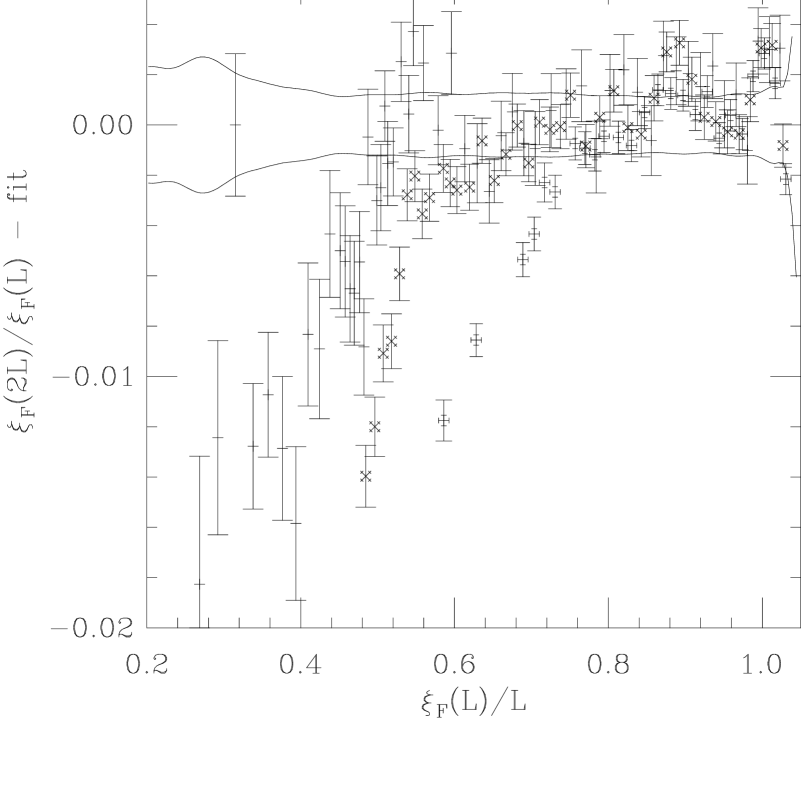
Figure 1: Deviation of points from fit to $F_{{\xi}_{F}}$ with $s=2$, $n=13$, $x_{min}=(\infty,\infty,\infty,0.14,0)$. Symbols indicate $L=8$ (+––$\tiny\vdash$$\tiny\dashv$), 16 ($\times$$\tiny\times$$\tiny\times$$\tiny\times$$\tiny\times$), 32 ($+$), 64 ($\times$), 128 ($\Box$), 256 ($\Diamond$). Error bars are one standard deviation. Curves near zero indicate statistical error bars ($\pm$ one standard deviation) on the function $F_{\xi_{F}}(x)$.

We found tentatively that for ${\cal O}=\xi_{F}^{(2nd)}$ a thirteenth-order fit (5.3) is indicated: see the last few rows of Table 5. We next sought to investigate the strength of the corrections to scaling: we performed the fit with the conservative choices $L_{min}=64$, $\xi_{min}=10$ and $n=13$, and plotted on an expanded vertical scale the deviations from this fit. The results are shown in Figure 1. Clearly, there are significant corrections to scaling in the regions $x\mathrel{\hbox to0.0pt{\lower 3.0pt\hbox{$\mathchar 536\relax$}\hss}\raise 2.0pt\hbox{$\mathchar 316\relax$}}0.84$ (resp. 0.64, 0.52, 0.14) when $L=8$ (resp. 16, 32, 64); but the corrections to scaling become negligible (within statistical error) at $x$ larger than this. To take account of this $x$-dependence of the corrections to scaling, we adopted a modified scheme for imposing lower cutoffs on $\xi(L)$ and $L$, as follows: For each lattice size $L$, we choose a value $x_{min}(L)$, and we allow into the fit only those data pairs $(\beta,L)$/$(\beta,2L)$ satisfying $x\equiv\xi(L)/L\geq x_{min}(L)$. Our method is thus specified by the five cut points $x_{min}(8)$, $x_{min}(16)$, $x_{min}(32)$, $x_{min}(64)$, $x_{min}(128)$ along with the interpolation order $n$. We shall always choose $x_{min}(64)=0.14$ and $x_{min}(128)=0$, and shall thus omit them from the tables.

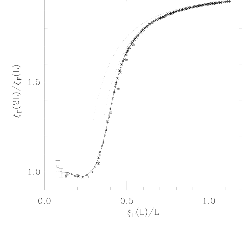
Figure 2: $\xi_{F}(\beta,2L)/\xi_{F}(\beta,L)$ versus $\xi_{F}(\beta,L)/L$. Symbols indicate $L=8$ (+––$\tiny\vdash$$\tiny\dashv$), 16 ($\times$$\tiny\times$$\tiny\times$$\tiny\times$$\tiny\times$), 32 ($+$), 64 ($\times$), 128 ($\Box$). Error bars are one standard deviation. Solid curve is a thirteenth-order fit in (5.3), with $x_{min}=(\infty,0.90,0.65,0.14,0)$ for $L=(8,16,32,64,128)$. Dotted curves are the perturbative prediction (LABEL:xiF_FSS_PT) through orders $1/x^{2}$ (upper curve) and $1/x^{4}$ (lower curve).

We next sought to investigate systematically the $\chi^{2}$ of the fits, as a function of the cut points $x_{min}(L)$ and the interpolation order $n$; some typical results are collected in Table 5. A reasonable $\chi^{2}$ is obtained when $n\geq 13$ and $x_{min}\geq(0.80,0.70,0.60,0.14,0)$ for $L=(8,16,32,64,128)$. Our preferred fit is $n=13$ and $x_{min}=(\infty,0.90,0.65,0.14,0)$: see Figure 2, where we compare also with the order-$1/x^{2}$ and order-$1/x^{4}$ perturbative predictions (LABEL:xiF_FSS_PT). This fit has $\chi^{2}=60.85$ (90 DF, level = 99.2%).

We then used this preferred fit to extrapolate the data to infinite volume. The extrapolated values $\xi_{F,\infty}^{(2nd)}$ from different lattice sizes at the same $\beta$ are consistent within statistical errors: only one of the 58 $\beta$ values has an ${\cal R}$ that is too large at the 5% level; and summing all $\beta$ values we have ${\cal R}=64.28$ (103 DF, level = 99.9%).

Both the $\chi^{2}$ and ${\cal R}$ values are unusually small; we don’t know why. Perhaps we have somewhere overestimated our statistical errors by about 25%.

In Table 6 we show the extrapolated values $\xi_{F,\infty}^{(2nd)}$ from our preferred fit and from some alternative fits, together with the propagated statistical error bars [including errors of type (i)+(ii)+(iii)]. The deviations between the different acceptable fits (those in italics or sans-serif), if larger than the statistical errors, can serve as a rough estimate of the remaining systematic errors due to corrections to scaling. The statistical errors on $\xi_{F,\infty}^{(2nd)}$ in our preferred fit are of order 0.6% (resp. 0.8%, 1.2%, 1.4%, 1.5%) at $\xi_{F,\infty}\approx 10^{2}$ (resp. $10^{3}$, $10^{4}$, $10^{5}$, $4\times 10^{5}$). The systematic errors are smaller than the statistical errors (anywhere from 0.1 to 0.9 times as large) for $\beta\mathrel{\hbox to0.0pt{\lower 3.0pt\hbox{$\mathchar 536\relax$}\hss}\raise 2.0pt\hbox{$\mathchar 316\relax$}}3.60$, and slightly larger than the statistical errors (by a factor 1–2 times as large) for $\beta\mathrel{\hbox to0.0pt{\lower 3.0pt\hbox{$\mathchar 536\relax$}\hss}\raise 2.0pt\hbox{$\mathchar 318\relax$}}3.60$. The statistical errors at different $\beta$ are strongly positively correlated.

Now we report the results for the observables $\chi_{F}$, $\xi_{A}^{(2nd)}$ and $\chi_{A}$.

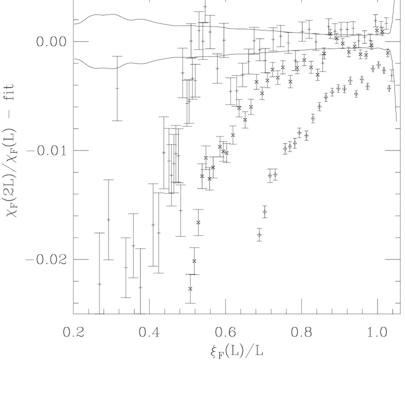
Figure 3: Deviation of points from fit to $F_{{\chi}_{F}}$ with $s=2$, $n=15$, $x_{min}=(\infty,\infty,\infty,0.14,0)$. Symbols indicate $L=8$ (+––$\tiny\vdash$$\tiny\dashv$), 16 ($\times$$\tiny\times$$\tiny\times$$\tiny\times$$\tiny\times$), 32 ($+$). Error bars are one standard deviation. Curves near zero indicate statistical error bars ($\pm$ one standard deviation) on the function $F_{\chi_{F}}(x)$.

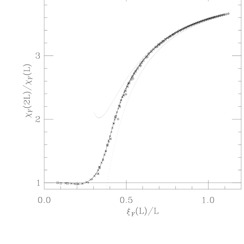
Figure 4: $\chi_{F}(\beta,2L)/\chi_{F}(\beta,L)$ versus $\xi_{F}(\beta,L)/L$. Symbols indicate $L=8$ (+––$\tiny\vdash$$\tiny\dashv$), 16 ($\times$$\tiny\times$$\tiny\times$$\tiny\times$$\tiny\times$), 32 ($+$), 64 ($\times$), 128 ($\Box$). Error bars are one standard deviation. Solid curve is a fifteenth-order fit in (5.3), with $x_{min}=(\infty,\infty,0.80,0.14,0)$ for $L=(8,16,32,64,128)$. Dotted curves are the perturbative prediction (LABEL:chiF_FSS_PT) through orders $1/x^{2}$ (lower curve) and $1/x^{4}$ (upper curve).

For ${\cal O}=\chi_{F}$ we observed tentatively that a fifteenth-order fit (5.3) is indicated: see Table 7. There are significant corrections to scaling for all $x$ when $L=8$, and in the regions $x\mathrel{\hbox to0.0pt{\lower 3.0pt\hbox{$\mathchar 536\relax$}\hss}\raise 2.0pt\hbox{$\mathchar 316\relax$}}0.85$ (resp. 0.50) when $L=16$ (resp. 32): see the deviations plotted in Figure 3. Our preferred fit is $n=15$ and $x_{min}=(\infty,\infty,0.80,0.14,0)$ for $L=(8,16,32,64,128)$: see Figure 4, where we compare also with the order-$1/x^{2}$ and order-$1/x^{4}$ perturbative predictions (LABEL:chiF_FSS_PT). This fit has $\chi^{2}=62.74$ (66 DF, level = 59.1%). In order to extrapolate $\chi_{F}(L)$ to infinite volume, we have to know both $F_{\xi_{F}}(x;s)$ and $F_{\chi_{F}}(x;s)$; but our preferred fit for $\chi_{F}$ requires a more stringent cut in $x_{min}$ than does our preferred fit for $\xi_{F}$. Therefore, to ensure the trustworthiness of the extrapolated values $\chi_{F,\infty}$, we enforce the more stringent cut on both observables: $x_{min}=(\infty,\infty,0.80,0.14,0)$. For $\xi_{F}$ we use the interpolation order $n=13$, while for $\chi_{F}$ we use $n=15$. The extrapolated values from different lattice sizes at the same $\beta$ are consistent within statistical errors: only one of the 58 $\beta$ values has an ${\cal R}$ that is too large at the 5% level; and summing all $\beta$ values we have ${\cal R}=58.32$ (81 DF, level = 97%). In Table 8 we show the extrapolated values $\chi_{F,\infty}$ from our preferred fit and from some alternative fits. The statistical errors on $\chi_{F,\infty}$ in our preferred fit are of order 0.6% (resp. 2.2%, 2.9%, 3.6%, 4.1%) at $\xi_{F,\infty}\approx 10^{2}$ (resp. $10^{3}$, $10^{4}$, $10^{5}$, $4\times 10^{5}$). The systematic errors are smaller than the statistical errors (anywhere from 0.07 to 0.8 times as large) for $\beta\mathrel{\hbox to0.0pt{\lower 3.0pt\hbox{$\mathchar 536\relax$}\hss}\raise 2.0pt\hbox{$\mathchar 316\relax$}}3.45$, and slightly larger than the statistical errors (by a factor 1–2.4 times as large) for $\beta\mathrel{\hbox to0.0pt{\lower 3.0pt\hbox{$\mathchar 536\relax$}\hss}\raise 2.0pt\hbox{$\mathchar 318\relax$}}3.60$.

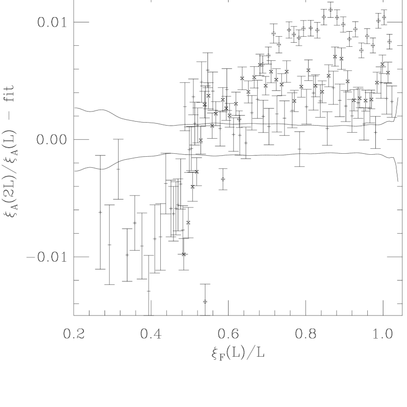
Figure 5: Deviation of points from fit to $F_{{\xi}_{A}}$ with $s=2$, $n=13$, $x_{min}=(\infty,\infty,\infty,0.14,0)$. Symbols indicate $L=8$ (+––$\tiny\vdash$$\tiny\dashv$), 16 ($\times$$\tiny\times$$\tiny\times$$\tiny\times$$\tiny\times$), 32 ($+$). Error bars are one standard deviation. Curves near zero indicate statistical error bars ($\pm$ one standard deviation) on the function $F_{\xi_{A}}(x)$.

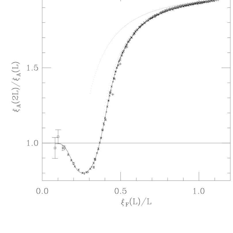
Figure 6: $\xi_{A}(\beta,2L)/\xi_{A}(\beta,L)$ versus $\xi_{F}(\beta,L)/L$. Symbols indicate $L=8$ (+––$\tiny\vdash$$\tiny\dashv$), 16 ($\times$$\tiny\times$$\tiny\times$$\tiny\times$$\tiny\times$), 32 ($+$), 64 ($\times$), 128 ($\Box$). Error bars are one standard deviation. Solid curve is a thirteenth-order fit in (5.3), with $x_{min}=(\infty,\infty,\infty,0.14,0)$ for $L=(8,16,32,64,128)$. Dotted curves are the perturbative prediction (LABEL:xiA_FSS_PT) through orders $1/x^{2}$ (upper curve) and $1/x^{4}$ (lower curve).

For ${\cal O}=\xi_{A}^{(2nd)}$ we observed tentatively that a thirteenth-order fit (5.3) is indicated: see Table 9. There are significant corrections to scaling for all $x$ when $L=8,16$ and probably also when $L=32$ (the correction is strongly negative for $x\mathrel{\hbox to0.0pt{\lower 3.0pt\hbox{$\mathchar 536\relax$}\hss}\raise 2.0pt\hbox{$\mathchar 316\relax$}}0.55$ and weakly positive when $x\mathrel{\hbox to0.0pt{\lower 3.0pt\hbox{$\mathchar 536\relax$}\hss}\raise 2.0pt\hbox{$\mathchar 318\relax$}}0.55$): see the deviations plotted in Figure 5. Our preferred fit is therefore $n=13$ and $x_{min}=(\infty,\infty,\infty,0.14,0)$ for $L=(8,16,32,64,128)$: see Figure 6, where we compare also with the order-$1/x^{2}$ and order-$1/x^{4}$ perturbative predictions (LABEL:xiA_FSS_PT). This fit has $\chi^{2}=32.82$ (50 DF, level = 97.1%). To extrapolate $\xi_{A}^{(2nd)}(L)$ to infinite volume we use the more stringent cut $x_{min}=(\infty,\infty,\infty,0.14,0)$ for both $\xi_{F}^{(2nd)}$ and $\xi_{A}^{(2nd)}$. The proper order of interpolation for this cut for both $\xi_{F}^{(2nd)}$ and $\xi_{A}^{(2nd)}$ is $n=13$ (see Tables 5 and 9). The extrapolated values from different lattice sizes at the same $\beta$ are consistent within statistical errors: only one of the 58 $\beta$ values has a ${\cal R}$ that is too large at the 5% level; and summing all $\beta$ values we have ${\cal R}=38.12$ (63 DF, level = 99.4%). In Table 10 we show the extrapolated values $\xi_{A,\infty}^{(2nd)}$ from our preferred fit and from some alternative fits. The statistical errors on $\xi_{A,\infty}^{(2nd)}$ in our preferred fit are of order 0.5% (resp. 1.3%, 2.3%, 2.9%, 3.5%) at $\xi_{F,\infty}\approx 10^{2}$ (resp. $10^{3}$, $10^{4}$, $10^{5}$, $4\times 10^{5}$). Since our preferred fit is the most conservative one possible (and all less conservative fits are bad), we are unable to say anything about the systematic errors.

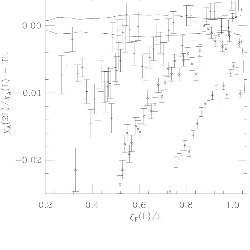
Figure 7: Deviation of points from fit to $F_{{\chi}_{A}}$ with $s=2$, $n=14$, $x_{min}=(\infty,\infty,\infty,0.14,0)$. Symbols indicate $L=8$ (+––$\tiny\vdash$$\tiny\dashv$), 16 ($\times$$\tiny\times$$\tiny\times$$\tiny\times$$\tiny\times$), 32 ($+$). Error bars are one standard deviation. Curves near zero indicate statistical error bars ($\pm$ one standard deviation) on the function $F_{\chi_{A}}(x)$.

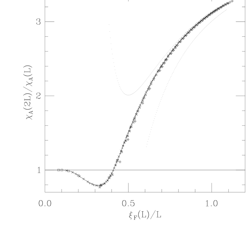
Figure 8: $\chi_{A}(\beta,2L)/\chi_{A}(\beta,L)$ versus $\xi_{F}(\beta,L)/L$. Symbols indicate $L=8$ (+––$\tiny\vdash$$\tiny\dashv$), 16 ($\times$$\tiny\times$$\tiny\times$$\tiny\times$$\tiny\times$), 32 ($+$), 64 ($\times$), 128 ($\Box$). Error bars are one standard deviation. Solid curve is a fourteenth-order fit in (5.3), with $x_{min}=(\infty,\infty,0.90,0.14,0)$ for $L=(8,16,32,64,128)$. Dotted curves are the perturbative prediction (LABEL:chiA_FSS_PT) through orders $1/x^{2}$ (lower curve) and $1/x^{4}$ (upper curve).

For ${\cal O}=\chi_{A}$ we observed tentatively that a fourteenth-order fit (5.3) is indicated: see Table 11. There are significant corrections to scaling for all $x$ when $L=8$, and in the regions $x\mathrel{\hbox to0.0pt{\lower 3.0pt\hbox{$\mathchar 536\relax$}\hss}\raise 2.0pt\hbox{$\mathchar 316\relax$}}0.84$ (resp. 0.64) when $L=16$ (resp. 32): see the deviations plotted in Figure 7. Our preferred fit is $n=14$ and $x_{min}=(\infty,\infty,0.90,0.14,0)$: see Figure 8, where we compare also with the order-$1/x^{2}$ and order-$1/x^{4}$ perturbative predictions (LABEL:chiA_FSS_PT). This fit has $\chi^{2}=40.31$ (62 DF, level = 98.5%). To extrapolate $\chi_{A}(L)$ to infinite volume we use more stringent fit $x_{min}=(\infty,\infty,0.90,0.14,0)$ for both $\xi_{F}^{(2nd)}$ and $\chi_{A}$, using $n=13$ for $\xi_{F}^{(2nd)}$ and $n=14$ for $\chi_{A}$. The extrapolated values from different lattice sizes at the same $\beta$ are consistent within statistical errors: none of the 58 $\beta$ values has an ${\cal R}$ that is too large at the 5% level; and summing all $\beta$ values we have ${\cal R}=46.86$ (75 DF, level = 99.6%). In Table 12 we show the extrapolated values $\chi_{A,\infty}$ from our preferred fit and from some alternative fits. The statistical errors on $\chi_{A,\infty}$ in our preferred fit are of order 0.3% (resp. 1.6%, 3.1%, 3.9%, 4.3%) at $\xi_{F,\infty}\approx 10^{2}$ (resp. $10^{3}$, $10^{4}$, $10^{5}$, $4\times 10^{5}$). The systematic errors are smaller than the statistical errors (anywhere from 0.05 to 0.5 times as large) for $\beta\mathrel{\hbox to0.0pt{\lower 3.0pt\hbox{$\mathchar 536\relax$}\hss}\raise 2.0pt\hbox{$\mathchar 316\relax$}}3.825$, and comparable to the statistical errors (anywhere from 0.75 to 1.9 times as large) for $\beta\mathrel{\hbox to0.0pt{\lower 3.0pt\hbox{$\mathchar 536\relax$}\hss}\raise 2.0pt\hbox{$\mathchar 318\relax$}}3.90$.

We also extrapolated the quantities $\chi_{F}/(\xi^{(2nd)}_{F})^{2}$ and $\chi_{A}/(\xi^{(2nd)}_{A})^{2}$. The reason for doing these extrapolations is that the errors in the infinite-volume estimates of the ratios are much smaller (at least 15 times for the fundamental sector and 7 times for the adjoint sector) than those obtained by direct extrapolation of numerator and denominator assuming independent errors. Besides, knowing the covariance of the statistical fluctuations on our estimates of $\chi(\beta,L)$ and $\xi^{(2nd)}(\beta,L)$, we can compute correctly the error bars of the extrapolated ratios; by contrast, if we extrapolate $\chi$ and $\xi^{(2nd)}$ separately, we are obliged either to make the false assumption of independent errors or else involve the triangle inequality — both of which lead to error bars that are gross overestimates. In any case, we observe that the central values are consistent within error bars with those obtained by separate extrapolation of the numerator and denominator.

For ${\cal O}=\chi_{F}/(\xi^{(2nd)}_{F})^{2}$ we observed tentatively that a thirteenth-order fit (5.3) is indicated. There are significant corrections to scaling for all $x$ when $L=8,16$, and in the regions $x\mathrel{\hbox to0.0pt{\lower 3.0pt\hbox{$\mathchar 536\relax$}\hss}\raise 2.0pt\hbox{$\mathchar 316\relax$}}0.6$ and $x\mathrel{\hbox to0.0pt{\lower 3.0pt\hbox{$\mathchar 536\relax$}\hss}\raise 2.0pt\hbox{$\mathchar 318\relax$}}0.8$ when $L=32$. Then, our preferred fit is $n=13$ and $x_{min}=(\infty,\infty,\infty,0.14,0)$. This fit has $\chi^{2}=22.37$ (50 DF, level = 99.7%). To extrapolate $\chi_{F}/(\xi^{(2nd)}_{F})^{2}$ to infinite volume we use the more stringent fit $x_{min}=(\infty,\infty,\infty,0.14,0)$ for both $\xi_{F}^{(2nd)}$ and $\chi_{F}/(\xi^{(2nd)}_{F})^{2}$, using $n=13$ for both. The extrapolated values from different lattice sizes at the same $\beta$ are consistent within statistical errors: no one of the 58 $\beta$ values has a ${\cal R}$ that is too large at the 5% level; and summing all $\beta$ values we have ${\cal R}=36.38$ (63 DF, level $>99.9\%$). The statistical errors on $\chi_{F}/(\xi^{(2nd)}_{F})^{2}$ in our preferred fit are of order 0.4% (resp. 0.5%, 0.6%, 0.7%, 0.7%) at $\xi_{F,\infty}\approx 10^{2}$ (resp. $10^{3}$, $10^{4}$, $10^{5}$, $4\times 10^{5}$). Since our preferred fit is the most conservative one possible (and all less conservative fits are bad), we are unable to say anything about the systematic errors.

For ${\cal O}=\chi_{A}/(\xi^{(2nd)}_{A})^{2}$ we observed tentatively that a sixteenth-order fit (5.3) is indicated. There are strong corrections to scaling for all $x$ when $L=8,16,32$, so our preferred fit is $n=16$ and $x_{min}=(\infty,\infty,\infty,0.14,0)$. This fit has $\chi^{2}=18.92$ (50 DF, level $>99.9\%$). To extrapolate $\chi_{A}/(\xi^{(2nd)}_{A})^{2}$ to infinite volume we use the more stringent fit $x_{min}=(\infty,\infty,\infty,0.14,0)$ for both $\xi_{F}^{(2nd)}$ and $\chi_{A}/(\xi^{(2nd)}_{A})^{2}$, using $n=13$ for $\xi_{F}^{(2nd)}$ and $n=16$ for $\chi_{A}/(\xi^{(2nd)}_{A})^{2}$. The extrapolated values from different lattice sizes at the same $\beta$ are consistent within statistical errors: no one of the 58 $\beta$ values has a ${\cal R}$ that is too large at the 5% level; and summing all $\beta$ values we have ${\cal R}=29.38$ (63 DF, level $>99.9\%$). The statistical errors on $\chi_{A}/(\xi^{(2nd)}_{A})^{2}$ in our preferred fit are of order 0.7% (resp. 0.9%, 1.2%, 1.4%, 1.4%) at $\xi_{F,\infty}\approx 10^{2}$ (resp. $10^{3}$, $10^{4}$, $10^{5}$, $4\times 10^{5}$). Since our preferred fit is the most conservative one possible (and all less conservative fits are bad), we are unable to say anything about the systematic errors.

5.2.2 Ratio $\xi_{F}^{(2nd)}(L)/\xi_{A}^{(2nd)}(L)$

In this subsection we discuss the finite-size-scaling curve for the ratio $\xi_{F}^{(2nd)}(L)/\xi_{A}^{(2nd)}(L)$. We fit to the Ansatz

$${\xi_{F}^{(2nd)}(L)\over\xi_{A}^{(2nd)}(L)}\;=\;a_{0}+a_{1}e^{-1/x}+a_{2}e^{-2/x}+\ldots+a_{n}e^{-n/x}\;,$$ (5.38)

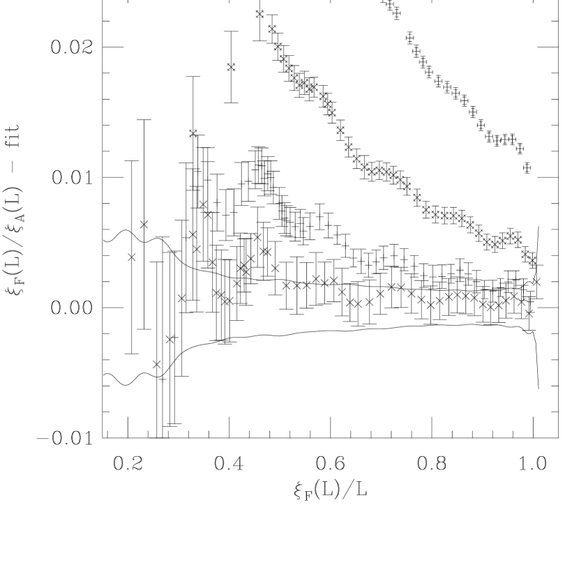
Figure 9: Deviation of points from fit (5.38) to $\xi_{F}(L)/\xi_{A}(L)$ with $n=15$, $\xi_{min}=10$ and $L_{min}=128$. Note the difference between this fit and previous ones: here we plot the finite-size-scaling curve for the ratio of $\xi_{F}$ and $\xi_{A}$ at the same $L$. Symbols indicate $L=8$ (+––$\tiny\vdash$$\tiny\dashv$), 16 ($\times$$\tiny\times$$\tiny\times$$\tiny\times$$\tiny\times$), 32 ($+$), 64($\times$). Error bars are one standard deviation. Curves near zero indicate statistical error bars ($\pm$ one standard deviation) on the fitting function.

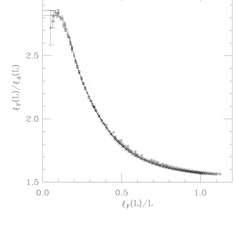
Figure 10: $\xi_{F}(\beta,L)/\xi_{A}(\beta,L)$ versus $\xi_{F}(\beta,L)/L$. Symbols indicate $L=8$ (+––$\tiny\vdash$$\tiny\dashv$), 16 ($\times$$\tiny\times$$\tiny\times$$\tiny\times$$\tiny\times$), 32 ($+$), 64 ($\times$), 128 ($\Box$), 256 ($\Diamond$). Error bars are one standard deviation. Solid curve reaching 2.817 at $x=0$ is a fourteenth-order fit in (5.38), with $L_{min}=128$, $\xi_{min}=10$. Solid curve reaching 2.859 at $x=0$ is a sixteenth-order fit in (5.40), also with $L_{min}=128$, $\xi_{min}=10$. Dotted curve is the perturbative prediction (3.25) through order $1/x^{2}$.

using $n=15$, $L_{min}=128$ and $\xi_{min}=10$. There are strong corrections to scaling for all $x$ when $L=8,16,32$ (Figure 9): these corrections are of positive sign and behave roughly as $L^{-\Delta}$ with $1\mathrel{\hbox to0.0pt{\lower 3.0pt\hbox{$\mathchar 536\relax$}\hss}\raise 2.0pt\hbox{$\mathchar 316\relax$}}\Delta\mathrel{\hbox to0.0pt{\lower 3.0pt\hbox{$\mathchar 536\relax$}\hss}\raise 2.0pt\hbox{$\mathchar 316\relax$}}2$. For $L=64$ these corrections to scaling are on the borderline of statistical significance, but the fact that they are nearly all positive (and are of the magnitude expected from extrapolation of the $L=32$ corrections) suggests that they are real. For all these reasons, we have chosen $L_{min}=128$. The resulting fit is shown in Figure 10 (lower solid curve); it has $\chi^{2}=21.45$ (47 DF, level $>99.9\%$). We thus estimate the limiting value as the value of $a_{0}$

$${\xi_{F,\infty}^{(2nd)}\over\xi_{A,\infty}^{(2nd)}}\;=\;a_{0}\;=\;2.817\pm 0.001$$ (5.39)

(68% confidence interval, statistical errors only). This estimate needs to be accompanied by one caveat: the paucity of our data with $L\leq 128$ in the region $x\mathrel{\hbox to0.0pt{\lower 3.0pt\hbox{$\mathchar 536\relax$}\hss}\raise 2.0pt\hbox{$\mathchar 316\relax$}}0.08$ makes the fit extremely sensitive to the assumed behavior at small $x$. Now, for $\xi_{A}^{(2nd)}$ (and hence also for the ratio $\xi_{A}^{(2nd)}/\xi_{F}^{(2nd)}$) there may be significant finite-size corrections of order $x^{2}$ at small $x$ (see footnote 22 in Section 5.1 above), which could be much larger than the $e^{-1/x}$ corrections assumed here. So we tried the alternative Ansatz

$${\xi_{F}^{(2nd)}(L)\over\xi_{A}^{(2nd)}(L)}\;=\;a^{\prime}_{0}+a^{\prime}_{1}x^{2}+a^{\prime}_{2}x^{4}+\ldots+a^{\prime}_{n}x^{2n}\;.$$ (5.40)

Using $n=16$, $L_{min}=128$ and $\xi_{min}=10$ we obtain an equally good fit ($\chi^{2}=13.86$, 46 DF, $\hbox{level}>99.9$%), which is shown as the upper solid curve in Figure 10. Note the different value of the limiting constant:

$${\xi_{F,\infty}^{(2nd)}\over\xi_{A,\infty}^{(2nd)}}\;=\;a^{\prime}_{0}\;=\;2.859\pm 0.002\;.$$ (5.41)

An alternative way of estimating the universal ratio ${\xi_{F,\infty}^{(2nd)}/\xi_{A,\infty}^{(2nd)}}$ is to use the separately extrapolated values for $\xi_{A,\infty}^{(2nd)}$ and $\xi_{F,\infty}^{(2nd)}$ (Tables 6 and 10) and simply form the ratio. Note that the deviations from constancy in ${\xi_{F,\infty}^{(2nd)}/\xi_{A,\infty}^{(2nd)}}$ are corrections to scaling (not to asymptotic scaling), and thus fall off as an inverse power of $\xi_{F,\infty}$ (most likely $\xi_{F,\infty}^{-2}$). Experience with other similar quantities suggests that good scaling will be observed for $\xi_{F,\infty}\mathrel{\hbox to0.0pt{\lower 3.0pt\hbox{$\mathchar 536\relax$}\hss}\raise 2.0pt\hbox{$\mathchar 318\relax$}}10$ (i.e. $\beta\mathrel{\hbox to0.0pt{\lower 3.0pt\hbox{$\mathchar 536\relax$}\hss}\raise 2.0pt\hbox{$\mathchar 318\relax$}}1.80$) or even smaller. Surprisingly, this does not occur here: if we use all data with $\xi_{F,\infty}\geq 10$ (i.e. $\beta\geq 1.80$), we obtain the estimate

$${\xi_{F,\infty}^{(2nd)}\over\xi_{A,\infty}^{(2nd)}}\;=\;2.8111\pm 0.0023\;,$$ (5.42)

but with a very poor goodness of fit ($\chi^{2}=127.68$, 55 DF, $\hbox{level}=10^{-7}$). In order to obtain a reasonable $\chi^{2}$, we have to restrict the fit to $\xi_{F,\infty}\geq 70$ (i.e. $\beta\geq 2.25$): we then get

$${\xi_{F,\infty}^{(2nd)}\over\xi_{A,\infty}^{(2nd)}}\;=\;2.798\pm 0.006$$ (5.43)

with $\chi^{2}=16.28$, 31 DF, $\hbox{level}=98.7$%. The discrepancy between (5.42) and (5.43) appears to be a real correction to scaling: its magnitude is very small ($\approx\!0.013$) and is consistent with a correction term $A\xi_{F,\infty}^{-2}$ with $A\sim 1$. We have two possible explanations for the horrible $\chi^{2}$ in (5.42):

• We have a large number of data points, each of which has a very small error bar; so very small corrections to scaling can became statistically significant.

• The extrapolated values $\xi_{F,\infty}^{(2nd)}/\xi_{A,\infty}^{(2nd)}$ at different $\beta$ are presumably positively correlated as a result of errors of type (iii) in the extrapolation, but we not taken account of this correlation here (see footnote 25); this could be causing the $\chi^{2}$ to appear larger than it really is. [On the other hand, we have overestimated the error bar on the ratio $\xi_{F,\infty}^{(2nd)}/\xi_{A,\infty}^{(2nd)}$ by assuming independent errors on $\xi_{F,\infty}^{(2nd)}$ and $\xi_{A,\infty}^{(2nd)}$, when in fact they are probably positively correlated; this would cause the $\chi^{2}$ to appear smaller than really is.]

In any case, the magnitude of this correction-to-scaling effect is very small, and we can simply fold the uncertainties into an enlarged error bar. One possible advantage of this method over the preceding one is that in the fit (5.3) to $\xi_{A}^{(2nd)}(2L)/\xi_{A}^{(2nd)}(L)$ we know the correct value at $x=0$ — namely, 1 — in contrast to the fit (5.38) where $a_{0}$ is unknown. As a result, the former fit is somewhat less sensitive to the assumed form of the small-$x$ corrections: if in Figures 2 and 6 we had fit to powers of $x^{2}$ instead of powers of $e^{-1/x}$, the resulting curve would have changed only slightly.

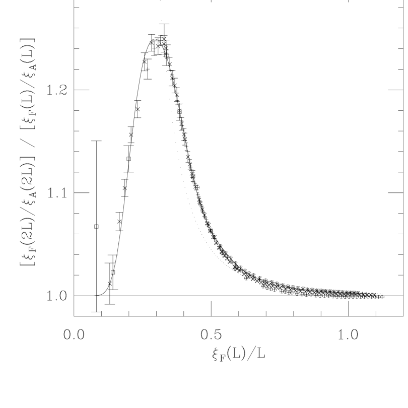
Figure 11: $R_{\xi}(\beta,2L)/R_{\xi}(\beta,L)$ versus $\xi_{F}^{(2nd)}(\beta,L)/L$, where $R_{\xi}\equiv\xi_{F}^{(2nd)}/\xi_{A}^{(2nd)}$. Symbols indicate $L=8$ (+––$\tiny\vdash$$\tiny\dashv$), 16 ($\times$$\tiny\times$$\tiny\times$$\tiny\times$$\tiny\times$), 32 ($+$), 64 ($\times$), 128 ($\Box$). Error bars are one standard deviation. Solid curve is a twelve-order fit in (5.3), with $x_{min}=(\infty,\infty,\infty,0.14,0)$ for $L=(8,16,32,64,128)$. Dotted curve is the perturbative prediction (3.24a,b) through order $1/x^{4}$ [at order $1/x^{2}$ it is identically 1].

Yet a third way of estimating ${\xi_{F,\infty}^{(2nd)}/\xi_{A,\infty}^{(2nd)}}$ is to treat the ratio ${\xi_{F}^{(2nd)}/\xi_{A}^{(2nd)}}$ as an observable ${\cal O}$ in its own right, and perform the fit (5.3) to ${\cal O}(2L)/{\cal O}(L)$ directly on it. This procedure is very similar to the preceding one, but has the advantage that the errors of type (iii) in the extrapolation — which are particularly important for the points at larger $\beta$ — are likely to partially cancel between $\xi_{F}^{(2nd)}$ and $\xi_{A}^{(2nd)}$. There are significant corrections to scaling for all $x$ when $L=8,16$; and for $L=32$ the corrections to scaling are positive and at least 0.5 standard deviations. Having presumably overestimated the error bars (see footnote 25), we assume that also the corrections to scaling are significant also for $L=32$. We therefore choose $x_{min}=(\infty,\infty,\infty)$, and use $n=12$: the resulting fit has $\chi^{2}=25.06$ (51 DF, level = 99.9%) and is shown in Figure 11. The extrapolated values from different lattice sizes at the same $\beta$ are consistent within statistical errors: two of the 58 $\beta$ values have a $\chi^{2}$ too large at the 5% level; and summing all $\beta$ values we have ${\cal R}=35.66$ (63 DF, level = 99.8%). Comparing the estimates of ${\xi_{F,\infty}^{(2nd)}/\xi_{A,\infty}^{(2nd)}}$ from different $\beta$ for consistency with a constant, we find a very large $\chi^{2}$ (confidence level $<2$%) no matter what cutoff $\beta_{min}$ we impose. Presumably these discrepancies arise from the correction to scaling in the $L=64$ points, which we discarded in the fits (5.38) and (5.40) but cannot afford to discard here. For this reason we believe the result obtained by this approach

$${\xi_{F,\infty}^{(2nd)}\over\xi_{A,\infty}^{(2nd)}}\;\approx\;2.79\pm 0.01\;,$$ (5.44)

to be less reliable than the estimate (5.43).

It is not clear to us whether (5.39), (5.41) or (5.43) is the more reliable estimate. A reasonable compromise would be to take

$${\xi_{F,\infty}^{(2nd)}\over\xi_{A,\infty}^{(2nd)}}\;\approx\;2.82\pm 0.05$$ (5.45)

as our “best estimate”; here we have increased the error bar to take account of the systematic uncertainties in the extrapolation.

5.2.3 Relative Variance-Time Product

Finally, let us discuss the efficiency of our extrapolation method for this model, as reflected in the scaling behavior (5.7) of the relative variance-time product (RVTP). We would like to test the theoretical predictions presented in Section 5.1.2, and in particular to determine the scaling functions ${\cal F}_{\xi}(z)$, $K_{\xi}(z)$, $\bar{v}(z)$, $v(z)$, $\bar{g}_{\Delta}(z)$ and $G_{\xi}(z)$ arising in that theory.

The functions ${\cal F}_{\xi}(z)$ and $K_{\xi}(z)$ [defined in (5.9)/(5.13)] can be easily obtained from the fitted finite-size-scaling function $F_{\xi}(x;2)$. Indeed, using the obvious recursion relation

$$F_{\xi}(x;s^{2})\;=\;F_{\xi}(F_{\xi}(x;s)/s;s)\,F_{\xi}(x;s)$$ (5.46)

one can compute numerically $F_{\xi}(x;\infty)$. Then, from $z=xF_{\xi}(x;\infty)$, one determines $x={\cal F}_{\xi}(z)$ and thence $K_{\xi}(z)$. Of course, the functions ${\cal F}_{\xi}(z)$ and $K_{\xi}(z)$ have the predicted logarithmic growths (5.16)/(5.17) at large $z$, because $F_{\xi}(x;2)$ has the predicted perturbative behavior at large $x$.

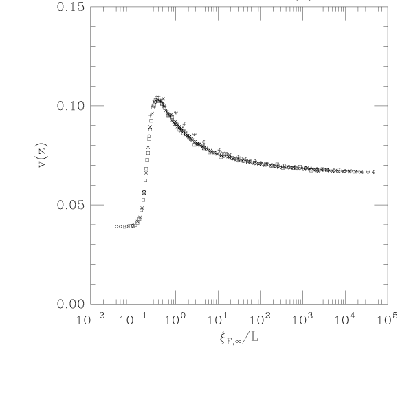
Figure 12: The scaling functions $\bar{v}(z)$ and $v(z)$ plotted versus $z\equiv\xi_{F,\infty}/L$, for the $SU(3)$ chiral model. Symbols indicate $L=8$ (+––$\tiny\vdash$$\tiny\dashv$), 16 ($\times$$\tiny\times$$\tiny\times$$\tiny\times$$\tiny\times$), 32 ($+$), 64 ($\times$), 128 ($\Box$), 256 ($\Diamond$). Note that $\bar{v}(z)\sim 1$ and $v(z)\sim\log^{2}z$ as $z\to\infty$.

Next we determined the functions $\bar{v}(z)$ and $v(z)$ controlling the static variance of the observable $\Delta$ [defined in (5.20)]: see Figure 12. Again we observe an excellent scaling, modified only by small corrections to scaling for the smallest lattices. We see that $\bar{v}(z)$ tends to a nonzero constant as $z\to\infty$, while $v(z)\sim\log^{2}z$. (A plot of $v(z)^{1/2}$ versus $\log z$ shows an excellent straight line at large $z$.)

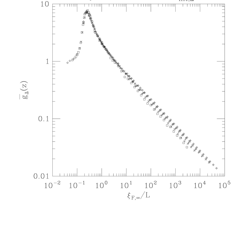
Figure 13: The dynamic scaling function $\bar{g}_{\Delta}(z)$ plotted versus $z\equiv\xi_{F,\infty}/L$, for the $SU(3)$ chiral model using the MGMC algorithm. Here $z_{int,\Delta}=0.45$. Symbols indicate $L=8$ (+––$\tiny\vdash$$\tiny\dashv$), 16 ($\times$$\tiny\times$$\tiny\times$$\tiny\times$$\tiny\times$), 32 ($+$), 64 ($\times$), 128 ($\Box$), 256 ($\Diamond$). Note that $\bar{g}_{\Delta}(z)\sim z^{-0.45}$ as $z\to\infty$.

Next we studied $\bar{g}_{\Delta}(z)$ [defined in (5.22)], which is the dynamic finite-size-scaling function for the autocorrelation time $\tau_{int,\Delta}$ in the MGMC algorithm. We varied the dynamic critical exponent $z_{int,\Delta}$ until we got a good fit: see Figure 13, where we have taken $z_{int,\Delta}=0.45$. We observe an excellent scaling, albeit with moderately strong corrections to scaling for the smallest lattices at large $z$. The large-$z$ behavior is approximately $\bar{g}_{\Delta}(z)\sim z^{-0.45}$, as predicted.

Finally, we determined the RVTP scaling function $G_{\xi}(z)$ using the relation

$$G_{\xi}(z)\;=\;{N_{iter}K_{\xi}(z)^{2}\over z^{2}\xi_{\infty}(\beta)^{z_{int,\Delta}}}\,{\hbox{\rm Var}(\xi(\beta,L))\over\xi(\beta,L)^{2}}\;,$$ (5.47)

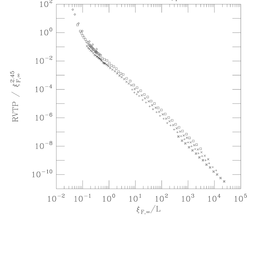
Figure 14: Scaling plot (5.7) for the relative variance-time product (RVTP), obtained using the fit $F_{{\xi}_{F}}$ with $s=2$, $n=13$, $x_{min}=(\infty,0.90,0.65,0.14,0)$. Symbols indicate $L=16$ ($\times$$\tiny\times$$\tiny\times$$\tiny\times$$\tiny\times$), 32 ($+$), 64 ($\times$), 128 ($\Box$), 256 ($\Diamond$).

where $\hbox{\rm Var}(\xi(\beta,L))$ is the variance of our Monte Carlo estimate of $\xi(\beta,L)$ as obtained from a run of $N_{iter}$ iterations. The resulting function $G_{\xi}(z)$ for $z_{int,\Delta}=0.45$ is shown in Figure 14. The scaling is reasonably good, though far from perfect. The large-$z$ behavior is in fairly good agreement with the prediction (5.28) that $G_{\xi}(z)\sim z^{-2.45}(\log z)^{2}$, but there are some discrepancies: indeed, a somewhat better fit at large $z$ is obtained with $z^{-2.45}(\log z)^{4}$. It is therefore possible that our analysis in Section 5.1.2 has somewhere overlooked an additional source of logarithms.

As a practical matter, the rapid decrease of $G_{\xi}(z)$ means that runs at $\xi_{\infty}/L\sim 10^{4}$ using the extrapolation method are roughly a factor $10^{9}$ more efficient [as regards statistical errors of types (i) + (ii)] than the traditional approach using runs at $\xi_{\infty}/L\approx 1/6$.

5.3 Data Analysis: Comparison with Perturbation Theory

Let us now compare our data with the predictions of weak-coupling perturbation theory, and in particular with the asymptotic-freedom scenario. In Section 5.3.1 we look at the local quantities (viz. the energies). In Section 5.3.2 we compare the raw (finite-$L$) data for the long-distance quantities (correlation lengths and susceptibilities) with the predictions of finite-volume perturbation theory [cf. (B.24)]. Finally, in Sections 5.3.3–5.3.6 we compare the extrapolated ($L=\infty$) data for the long-distance quantities with the asymptotic-freedom predictions (3.3)–(3.6).

5.3.1 Local Quantities

We can compare the fundamental energy $E_{F}$ with the one-loop, two-loop and three-loop perturbative predictions (3.1), and the adjoint energy $E_{A}$ with the one-loop and two-loop predictions (3.2). In each case we use the value measured on the largest lattice available (which is usually $L=128$); we define the error bar to be the statistical error (one standard deviation) on the largest lattice plus the discrepancy between the values on the largest and second-largest lattices (this is a conservative estimate of the systematic error due to finite-size effects). For $E_{F}$ the finite-size corrections are between 0.000035 and 0.000132 (10–20 times larger than the statistical errors) for $\beta\mathrel{\hbox to0.0pt{\lower 3.0pt\hbox{$\mathchar 536\relax$}\hss}\raise 2.0pt\hbox{$\mathchar 318\relax$}}2.60$, and between 0.0001 and 0.0005 (20–50 times larger than the statistical errors) for $1.95\mathrel{\hbox to0.0pt{\lower 3.0pt\hbox{$\mathchar 536\relax$}\hss}\raise 2.0pt\hbox{$\mathchar 316\relax$}}\beta\mathrel{\hbox to0.0pt{\lower 3.0pt\hbox{$\mathchar 536\relax$}\hss}\raise 2.0pt\hbox{$\mathchar 316\relax$}}2.60$. For $E_{A}$ the finite-size corrections are between 0.000065 and 0.000153 (10–20 times larger than the statistical errors) for $\beta\mathrel{\hbox to0.0pt{\lower 3.0pt\hbox{$\mathchar 536\relax$}\hss}\raise 2.0pt\hbox{$\mathchar 318\relax$}}2.60$, and between 0.0002 and 0.0006 (20–50 times larger than the statistical errors) for $1.95\mathrel{\hbox to0.0pt{\lower 3.0pt\hbox{$\mathchar 536\relax$}\hss}\raise 2.0pt\hbox{$\mathchar 316\relax$}}\beta\mathrel{\hbox to0.0pt{\lower 3.0pt\hbox{$\mathchar 536\relax$}\hss}\raise 2.0pt\hbox{$\mathchar 316\relax$}}2.60$.

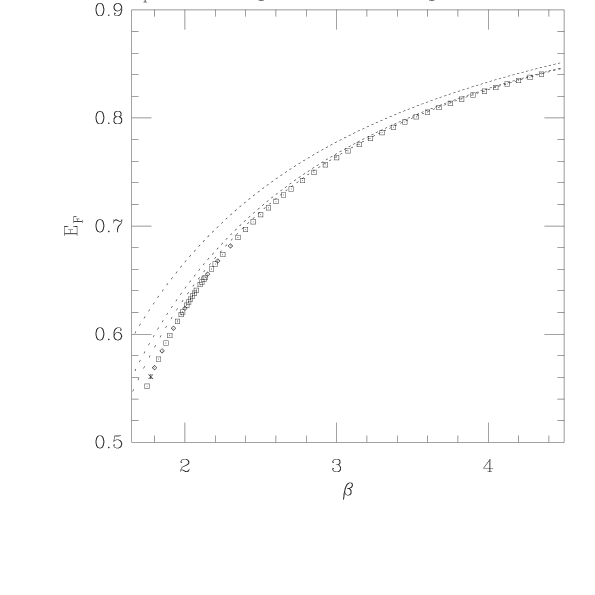
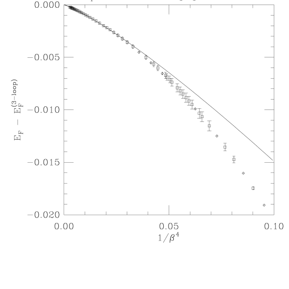
Figure 15: (a) Fundamental energy $E_{F}$ versus $\beta$. Each point comes from the largest lattice available at a given $\beta$: $L=64$ ($\times$), $L=128$ ($\Box$) or $L=256$ ($\Diamond$). Error bars (usually invisible) are statistical error (one standard deviation) plus a conservative estimate of the systematic error due to finite-size corrections. Dashed curves are the perturbative prediction (3.1) through orders $1/\beta$ (top curve), $1/\beta^{2}$ (middle curve), and $1/\beta^{3}$ (bottom curve). (b) Deviations of fundamental energy $E_{F}$ from three-loop perturbative prediction (3.1), plotted versus $1/\beta^{4}$. Solid curve corresponds to the fit $E_{F}-E_{F}^{(3-loop)}=k_{4}/\beta^{4}+k_{5}/\beta^{5}$ for $\beta\geq 2.35$.

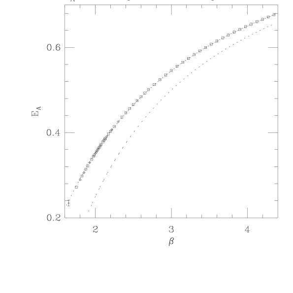
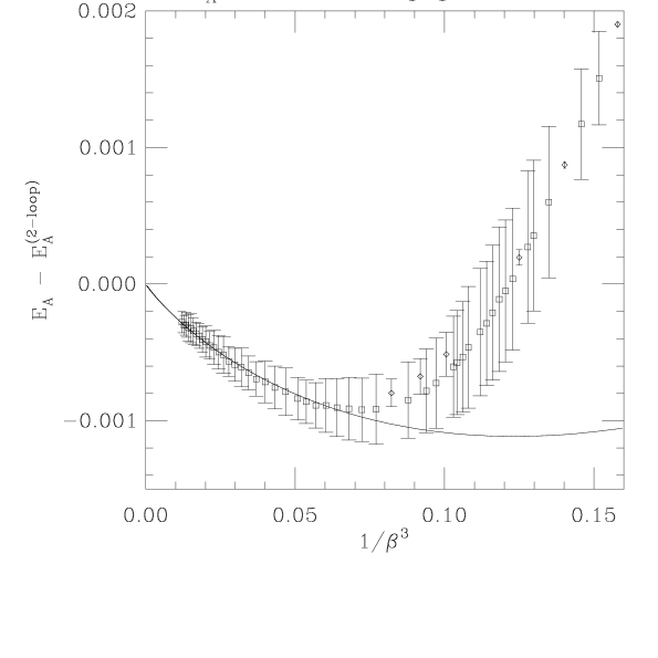
Figure 16: (a) Adjoint energy $E_{A}$ versus $\beta$. Each point comes from the largest lattice available at a given $\beta$: $L=64$ ($\times$), $L=128$ ($\Box$) or $L=256$ ($\Diamond$). Error bars (usually invisible) are statistical error (one standard deviation) plus a conservative estimate of the systematic error due to finite-size corrections. Dashed curves are the perturbative prediction (3.2) through orders $1/\beta$ (lower curve) and $1/\beta^{2}$ (upper curve). (b) Deviations of fundamental energy $E_{A}$ from two-loop perturbative prediction (3.2), plotted versus $1/\beta^{3}$. Solid curve corresponds to the fit $E_{A}-E_{A}^{(2-loop)}=k_{3}/\beta^{3}+k_{4}/\beta^{4}$ for $\beta\geq 2.35$.

Both the fundamental and adjoint energies are in reasonably good agreement with the perturbative predictions: see Figures 15(a) and 16(a). Furthermore, we can use the observed deviations from these perturbative predictions to obtain crude estimates of the next perturbative coefficients (which we hope someone will calculate in the near future). In Figure 15(b) we plot $E_{F}-E_{F}^{(3-loop)}$ versus $1/\beta^{4}$. The limiting slope suggests a four-loop coefficient of order $-0.05$ to $-0.1$. If we fit $E_{F}-E_{F}^{(3-loop)}=k_{4}\beta^{-4}+k_{5}\beta^{-5}$, a reasonable fit is obtained if we restrict attention to the points with $\beta\geq 2.35$, and we get $k_{4}=-0.02430\pm 0.00942$, $k_{5}=-0.222\pm 0.026$. Unfortunately, this fit would imply that $|k_{5}/\beta^{5}|$ is more than twice as large as $|k_{4}/\beta^{4}|$ even at our largest value of $\beta$ ($=4.35$), so that the extrapolation to $\beta=\infty$ cannot be taken seriously. All we can conclude is that: (a) $k_{4}$ is somewhere in the range from $-0.02$ to $-0.10$; and (b) if $k_{4}$ turns to be closer to the former value, then $k_{5}$ must be negative and of rather large magnitude (of order $-0.10$ or $-0.20$). These estimates can be compared to the known values of $k_{1}=-2/3$, $k_{2}=-0.0972222$, $k_{3}=-0.0679225$.

We proceed similarly for the adjoint energy. In Figure 16(b) we plot $E_{A}-E_{A}^{3-loop}$ versus $1/\beta^{3}$. The limiting slope suggests a three-loop coefficient of order $-0.02$. If we fit $E_{A}-E_{A}^{3-loop}=l_{3}\beta^{-3}+l_{4}\beta^{-4}$, a reasonable fit is obtained if we restrict attention to the points with $\beta\geq 2.35$, and we get $l_{3}=-0.0361\pm 0.0046$, $l_{4}=0.054\pm 0.013$. However, these error bars should not be taken seriously, as we are neglecting terms of order $\beta^{-5}$, $\beta^{-6}$, etc. In any case, it is worth comparing these estimates to the known values $l_{1}=-3/2$, $l_{2}=0.40625$.

5.3.2 Comparison of Long-Distance Quantities with Finite-Volume Perturbation Theory

Let us next compare the finite-volume Monte Carlo data ${\cal O}(\beta,L)$ for the long-distance observables ${\cal O}=\xi_{\#}^{(2nd)}$ and $\chi_{\#}$ with the predictions (B.24) of finite-volume perturbation theory ($\beta\to\infty$ at fixed $L<\infty$). The expansions (B.24) give $\chi_{\#}$ through order $1/\beta^{2}$, and $\xi_{\#}$ through order $1/\beta$; they are derived from the expansions (B.22), which give $G_{\#}$ through order $1/\beta^{2}$. We restrict attention to $8\leq L\leq 128$, as our very few $L=256$ data points are all far from the perturbative regime (they all have $\beta\leq 2.30$ and $x\equiv\xi_{F}^{(2nd)}(L)/L<0.33$).

We begin with the correlation lengths $\xi_{F}^{(2nd)}$ and $\xi_{A}^{(2nd)}$. For these observables, the expansion is of the form

$$\xi_{\#}^{(2nd)}(\beta,L)\;=\;A\,\beta^{1/2}\,L\left[1\,-\,{A_{1}(L)\over\beta}\,-\,O(\beta^{-2})\right]$$ (5.48)

with $A_{1}(L)\sim\log L$ at large $L$ [cf. (LABEL:fss:xi1)]. Luckily, $A_{1}(L)$ is not too large for these two expansions: for $\xi_{F}^{(2nd)}$ it ranges from $\approx\!0.48$ at $L=8$ to $\approx\!0.80$ at $L=128$, while for $\xi_{A}^{(2nd)}$ it ranges from $\approx\!0.61$ at $L=8$ to $\approx\!0.92$ at $L=128$. As a result, the first-order perturbation correction in the range of interest ($2\mathrel{\hbox to0.0pt{\lower 3.0pt\hbox{$\mathchar 536\relax$}\hss}\raise 2.0pt\hbox{$\mathchar 316\relax$}}\beta\mathrel{\hbox to0.0pt{\lower 3.0pt\hbox{$\mathchar 536\relax$}\hss}\raise 2.0pt\hbox{$\mathchar 316\relax$}}4$) is of modest size, namely 10–40%. Furthermore, the discrepancy between the Monte Carlo data and the perturbative predictions,

$$R_{2}(\beta,L)\;\equiv\;{\xi_{\#}^{(2nd)}(\beta,L)\over A\,\beta^{1/2}\,L}\,-\,\left[1\,-\,{A_{1}(L)\over\beta}\right]\;,$$ (5.49)

is smaller than this by a factor of 2–10: see Tables 13 and 14.

Let us now examine more closely the behavior of the remainder term $R_{2}(\beta,L)$. Heuristically we would expect the remainder in first-order perturbation theory to be of the same order of magnitude as the second-order perturbative correction, i.e. of order $-A_{2}(L)/\beta^{2}\sim(\log L)^{2}/\beta^{2}$. Let us therefore define

$$\widetilde{R}_{2}(\beta,L)\;\equiv\;{\beta^{2}\over(\log L)^{2}}\,R_{2}(\beta,L)\;.$$ (5.50)

We would like to know whether or not $|\widetilde{R}_{2}(\beta,L)|$ is uniformly bounded in $\beta\geq\hbox{some }\beta_{0}$ and $L\geq\hbox{some }L_{0}$, as it should be if the perturbation series is to be “well-behaved”.

We can say something rigorously in three different regimes:

• As $\beta\to\infty$ at fixed $L<\infty$, we have $\lim\limits_{\beta\to\infty}\beta^{2}R_{2}(\beta,L)=-A_{2}(L)$ [with corrections of order $1/\beta$], and hence $\lim\limits_{L\to\infty}\lim\limits_{\beta\to\infty}\widetilde{R}_{2}(\beta,L)=-A_{22}=-A_{11}^{2}/2$ [cf. (LABEL:fss:AB_relations_A)].

• As $L\to\infty$ at fixed $\beta<\infty$, we have $\lim\limits_{L\to\infty}(\log L)^{-1}R_{2}(\beta,L)=A_{11}/\beta$, and hence $\lim\limits_{L\to\infty}\widetilde{R}_{2}(\beta,L)=0$ [with corrections of order $1/\log L$].

• Since $\xi(\beta,L)\geq 0$, we have $R_{2}(\beta,L)\geq[A_{1}(L)/\beta]-1$ for all $\beta,L$. In particular, along any curve $\beta=cA_{1}(L)$ with $c>0$ [which makes sense at least for large $\beta$ since $A_{11}>0$], we can conclude that $\widetilde{R}_{2}(\beta,L)\geq c(1-c)A_{1}(L)^{2}/\log^{2}L$, which for large $L$ tends to $c(1-c)A_{11}^{2}$. For $0<c<1$ this proves that $\widetilde{R}_{2}(\beta,L)>0$ and provides a lower bound on its magnitude; for $c>1$ it constrains only how negative $\widetilde{R}_{2}(\beta,L)$ can get.

Furthermore, under the assumptions of the conventional wisdom, we can say something analytically in one sub-case of regime (iii):

• As $\beta,L\to\infty$ at fixed $x\equiv\xi_{F}^{(2nd)}(\beta,L)/L\neq 0,\infty$, we have

  $$\lim\limits_{00112233\begin{array}[]{c}\beta,L\to\infty\\ x\,\hbox{\scriptsize fixed}\,\neq 0,\infty\end{array}}\!{\beta\over\log L}\;=\;w_{0}\;=\;2A_{11}$$ (5.51)

  [corresponding to $c=2$ in regime (iii)] and

  $$\lim\limits_{00112233\begin{array}[]{c}\beta,L\to\infty\\ x\,\hbox{\scriptsize fixed}\,\neq 0,\infty\end{array}}\!\widetilde{R}_{2}(\beta,L)\;=\;-2A_{11}^{2}\;.$$ (5.52)

[This shows that the lower bound for regime (iii) is sharp when $c=2$.] Proof of (5.51)/(5.52): From asymptotic scaling (3.3) we have $\log\xi_{\infty}(\beta)=\beta/w_{0}+O(\log\beta)$ where $w_{0}=2A_{11}$ is the first coefficient of the RG beta-function [cf. (LABEL:fss:RGpertxi)/(B.11a)]. According to finite-size scaling (5.1), taking $\beta,L\to\infty$ at fixed $x\equiv\xi(\beta,L)/L\neq 0,\infty$ implies that $\xi_{\infty}(\beta)/L$ also converges to a limit $\neq 0,\infty$, so that in particular $\log\xi_{\infty}(\beta)/\log L\to 1$. This implies (5.51). On the other hand, $\xi(\beta,L)/[A\beta^{1/2}L]=x/[A\beta^{1/2}]$, which tends to zero as $\beta\to\infty$ at fixed $x$. It follows that $R_{2}(\beta,L)\to-{1\over 2}$, which together with (5.51) implies (5.52). Q.E.D. [This is somewhat strange: the limiting value of $\widetilde{R}_{2}(\beta,L)$ must behave in a highly non-monotonic way as we pass from regime (ii) through regime (iii)/(iii^′) to regime (i).]

We can use our Monte Carlo data to study the behavior of $\widetilde{R}_{2}(\beta,L)$. First of all, let us look at limit (i): We know that

$$A_{2}(L)\;=\;A_{22}\log^{2}L\,+\,A_{21}\log L\,+\,A_{20}\,+\,O\!\left({\log^{2}L\over L^{2}}\right)$$ (5.53)

with

$$A_{22}&={N^{2}\over 128\pi^{2}}\\ A_{21}={N^{2}\over 64\pi^{2}}\,+\,{N\over 8\pi}A_{10}$$ (5.54)

[cf. (B.11a,b) and (A.22)/(A.23)], where we have

$$A_{10}^{(F)}&={1\over 4}\left[NI_{1,fin}\,+\,{N^{2}-2\over 4N}\,+\,{N^{2}-2\over 2N}\left(4\pi^{2}I_{3,\infty}+{1\over 2\pi^{2}}\right)\right]\\ A_{10}^{(A)}={1\over 4}\left[NI_{1,fin}\,+\,{N^{2}-2\over 4N}\,+\,{3N\over 2}\left(4\pi^{2}I_{3,\infty}+{1\over 2\pi^{2}}\right)\right]$$ (5.55)

for the fundamental and adjoint sectors [see (B.27)–(B.31) for definitions]. Unfortunately $A_{20}^{(F)}$ and $A_{20}^{(A)}$ are unknown. We can use our Monte Carlo data to estimate $A_{2}^{(\#)}(L)$ for $L=8,16,32,64,128$; in this way we can test (5.53)–(5.55) and obtain a rough estimate of $A_{20}^{(\#)}$. The data are approximately converged for $L=8$, and suggest very roughly $A_{20}^{(F)}\approx 0.09$ and $A_{20}^{(A)}\approx 0.14$ (see the next-to-last column of Tables 13 and 14). The data for larger $L$ are at least consistent with convergence to these values.

In limit (ii), we see $|\widetilde{R}_{2}(\beta,L)|$ slowly decreasing as a function of $L$ when $L\ll\xi_{F,\infty}(\beta)$, then beginning to grow slightly when $L\sim\xi_{F,\infty}(\beta)$. We know that $|\widetilde{R}_{2}(\beta,L)|$ must ultimately decrease again to zero as $L\to\infty$, but our data do not allow us to observe this decrease (this is not surprising since the rate of convergence is only $1/\log L$).

Along the curves $x={\rm constant}$ [limit (iii^′)], $\widetilde{R}_{2}(\beta,L)$ stays bounded and is roughly consistent with convergence to the predicted value $-2A_{11}^{2}=N^{2}/(32\pi^{2})\approx-0.028497$.

In summary, our data in Tables 13 and 14 give no evidence of $\widetilde{R}_{2}(\beta,L)$ becoming unbounded in any region of the $(\beta,L)$-plane. It is of course still possible that $\widetilde{R}_{2}(\beta,L)$ does become unbounded in some region far from the one we have studied; this question needs ultimately to be resolved by a rigorous mathematical proof.

Let us now look at the susceptibilities $\chi_{F}$ and $\chi_{A}$, for which the expansion is of the form

$$\chi_{\#}(\beta,L)\;=\;B\,L^{2}\left[1\,-\,{B_{1}(L)\over\beta}\,-\,{B_{2}(L)\over\beta^{2}}\,-\,O(\beta^{-3})\right]$$ (5.56)

with $B_{1}(L)\sim\log L$ and $B_{2}(L)\sim(\log L)^{2}$ at large $L$. For $\chi_{F}$ the coefficient $B_{1}(L)$ is rather large, ranging from $\approx\!1.01$ at $L=8$ to $\approx\!2.19$ at $L=128$, while $B_{2}(L)$ is fairly small, ranging from $\approx\!0.04$ at $L=8$ to $\approx-0.43$ at $L=128$. As a result, the first-order perturbation corrections are quite large in the range of interest, but the second-order corrections are small; and the discrepancy between the Monte Carlo data and the second-order perturbative prediction is a factor 1–10 smaller than the second-order correction (see Table 15). For $\chi_{A}$, by contrast, both coefficients are very large: $B_{1}(L)$ ranges from $\approx\!2.28$ at $L=8$ to $\approx\!4.93$ at $L=128$, while $B_{2}(L)$ ranges from $\approx-1.39$ at $L=8$ to $\approx-7.75$ at $L=128$. As a result, both the first-order and second-order perturbation corrections are huge; nevertheless, the discrepancy between the Monte Carlo data and the second-order perturbative prediction is surprisingly small (see Table 16).

Let us define the discrepancy between the exact values and the second-order perturbative predictions,

$$S_{3}(\beta,L)\;\equiv\;{\chi_{\#}(\beta,L)\over BL^{2}}\,-\,\left[1\,-\,{B_{1}(L)\over\beta}\,-\,{B_{2}(L)\over\beta^{2}}\right]\;,$$ (5.57)

and the corresponding rescaled quantity

$$\widetilde{S}_{3}(\beta,L)\;\equiv\;{\beta^{3}\over(\log L)^{3}}\,S_{3}(\beta,L)\;.$$ (5.58)

Just as for the correlation lengths, we can prove rigorously the behavior in regimes (i)–(iii):

• As $\beta\to\infty$ at fixed $L<\infty$, we have $\lim\limits_{\beta\to\infty}\beta^{3}S_{3}(\beta,L)=-B_{3}(L)$, and hence $\lim\limits_{L\to\infty}\lim\limits_{\beta\to\infty}$ $\widetilde{S}_{3}(\beta,L)=-B_{33}$.

• As $L\to\infty$ at fixed $\beta<\infty$, we have $\lim\limits_{L\to\infty}(\log L)^{-2}S_{3}(\beta,L)=B_{22}/\beta$, and hence $\lim\limits_{L\to\infty}\widetilde{S}_{3}(\beta,L)=0$.

• Since $\chi(\beta,L)\geq 0$, we have $S_{3}(\beta,L)\geq[B_{1}(L)/\beta]+[B_{2}(L)/\beta^{2}]-1$ for all $\beta,L$. In particular, along any curve $\beta=cA_{1}(L)$ with $c>0$, we can conclude that (writing for simplicity only the $L\to\infty$ limit) we have $\widetilde{S}_{3}(\beta,L)\mathrel{\hbox to0.0pt{\lower 3.0pt\hbox{$\mathchar 536\relax$}\hss}\raise 2.0pt\hbox{$\mathchar 318\relax$}}c^{2}A_{11}^{2}B_{11}+cA_{11}B_{22}-c^{3}A_{11}^{3}=(c^{2}+c)A_{11}^{2}B_{11}-{{1\over 2}}cA_{11}B_{11}^{2}-c^{3}A_{11}^{3}$ [cf. (B.7b)]. Unfortunately, the sign of this lower bound is far from obvious.

Furthermore, the assumptions of the conventional wisdom imply that

• As $\beta,L\to\infty$ at fixed $x\equiv\xi_{F}^{(2nd)}(\beta,L)/L\neq 0,\infty$, we have

  $$\lim\limits_{00112233\begin{array}[]{c}\beta,L\to\infty\\ x\,\hbox{\scriptsize fixed}\,\neq 0,\infty\end{array}}\!\widetilde{S}_{3}(\beta,L)\;=\;6A_{11}^{2}B_{11}-A_{11}B_{11}^{2}-8A_{11}^{3}\;.$$ (5.59)

[This shows that the lower bound for regime (iii) is sharp when $c=2$.] Proof of (5.59): We have (5.51) as before. On the other hand, let us write

$${\chi(\beta,L)\over L^{2}}\;=\;{\chi(\beta,L)\over\chi(\beta,\infty)}\,{\chi(\beta,\infty)\over\xi(\beta,\infty)^{2}}\,\left({\xi(\beta,\infty)\over L}\right)^{2}\;.$$ (5.60)

By finite-size-scaling theory, the first and third factors on the right-hand side tend to finite constants as $\beta,L\to\infty$ at fixed $x$; while asymptotic scaling implies that the second factor scales as $\beta^{-\gamma_{0}/w_{0}}$, hence vanishes as $\beta\to\infty$ because $\gamma_{0}/w_{0}>0$. Using (5.51), we easily deduce (5.59). Q.E.D.

We can use our Monte Carlo data to study the behavior of $\widetilde{S}_{3}(\beta,L)$. First of all, let us look at limit (i): We know that

$$B_{3}(L)\;=\;B_{33}\log^{3}L\,+\,B_{32}\log^{2}L\,+\,B_{31}\log L\,+\,B_{30}\,+\,O\!\left({\log^{3}L\over L^{2}}\right)$$ (5.61)

with

$$B_{33}&={1\over 6}(\gamma_{0}^{3}-3w_{0}\gamma_{0}^{2}+2w_{0}^{2}\gamma_{0})\\ B_{32}={1\over 2}(w_{1}\gamma_{0}+2w_{0}\gamma_{1}^{lat}-2\gamma_{0}\gamma_{1}^{lat})\,+\,{B_{10}\over 2}(2w_{0}^{2}+\gamma_{0}^{2}-3w_{0}\gamma_{0})\\ B_{31}=\gamma^{lat}_{2}\,+\,B_{10}(w_{1}-\gamma^{lat}_{1})\,+\,B_{20}(2w_{0}-\gamma_{0})$$ (5.62)

where the RG coefficients $w_{0},w_{1},\gamma_{0},\gamma_{1}^{lat},\gamma^{lat}_{2}$ can be found in Appendix A, and the constants $B_{10}$ and $B_{20}$ can be extracted from Appendix B (the latter formulae are somewhat lengthy). We consider first $\chi_{F}$, because it is only for the fundamental sector that we know the value of $\gamma^{lat}_{2}$. Numerically, for $N=3$ we have $B_{33}^{(F)}\approx-0.0006967924$, $B_{32}^{(F)}\approx-0.0175782344$ and $B_{31}^{(F)}\approx 0.0679511385$. Unfortunately $B_{30}^{(F)}$ is unknown. We can use our Monte Carlo data to test (5.61)–(5.62) and obtain a rough estimate of $B_{30}^{(F)}$. The first thing to note is that $S_{3}(\beta,L)$ undergoes a curious change of sign as $L$ varies (see Table 15); but this increase is almost entirely accounted for by the known terms $B_{33}\log^{3}L+B_{32}\log^{2}L+B_{31}\log L$, which exhibit a similar sign change. The difference is much smaller in magnitude, and as a result the estimated $B_{30}^{(F)}$ is much smaller in magnitude than $\beta^{3}S_{3}(\beta,L)$ [see the next-to-last column of Table 15]. Unfortunately the estimates of $B_{30}^{(F)}$ are not well converged (the fluctuations at larger $L$ are statistical error); all we can say is that $B_{30}^{(F)}$ is very small, probably somewhere between $-0.1$ and $0.1$.

Likewise, in limits (ii) and (iii^′), we are unable to see the predicted convergence of $\widetilde{S}_{3}(\beta,L)$ to a limiting value, or to say whether $|\widetilde{S}_{3}(\beta,L)|$ appears to remain bounded. In any case, $|\widetilde{S}_{3}(\beta,L)|$ stays extremely small.

Finally, let us consider the adjoint susceptibility $\chi_{A}$, for which the known numerical values (for $N=3$) are $B_{33}^{(A)}\approx 0.0544244644$ and $B_{32}^{(A)}\approx-0.1358424235$. For $\chi_{A}$, the first-order perturbative corrections are enormous (50–110% even at our largest $\beta$), and the second-order corrections are quite large (7–40% even at the largest $\beta$): see Table 16. In view of this, the deviations from second-order perturbation theory are amazingly small: e.g. a fraction of a percent when the second-order term is as large as 20%, or 10–40% when the second-order term is 100% or more. Furthermore, these deviations are almost perfectly explained by the $B_{3}(L)/\beta^{3}$ term, as can be seen from the almost-constancy of $\widetilde{S}_{3}(\beta,L)$ as a function of $\beta$ at each fixed $L$. The values of $\widetilde{S}_{3}(\beta,L)$ vary significantly with $L$, but it is plausible that they are approaching their predicted limiting value $-B_{33}^{(A)}\approx-0.054$ as $L\to\infty$ (the corrections are, after all, of order $1/\log L$ with a relatively large coefficient $B_{32}^{(A)}$). We do not have any explanation for these incredibly accurate predictions from an a priori badly behaved perturbation series.

5.3.3 Fundamental Sector: Correlation Length

In the next four subsections we shall compare the extrapolated infinite-volume values ${\cal O}_{\infty}(\beta)$ for the long-distance observables ${\cal O}=\xi_{\#}^{(2nd)}$ and $\chi_{\#}$, as generated in Section 5.2.1, with the asymptotic-freedom predictions.

We begin by comparing the fundamental correlation length $\xi_{F}^{(2nd)}$ with the two-loop and three-loop perturbative predictions (3.3)/(3.9). In all cases, we use the extrapolated data from our preferred fit: see Table 6, estimate $(\infty,0.90,0.65)$.

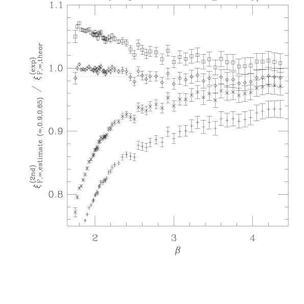
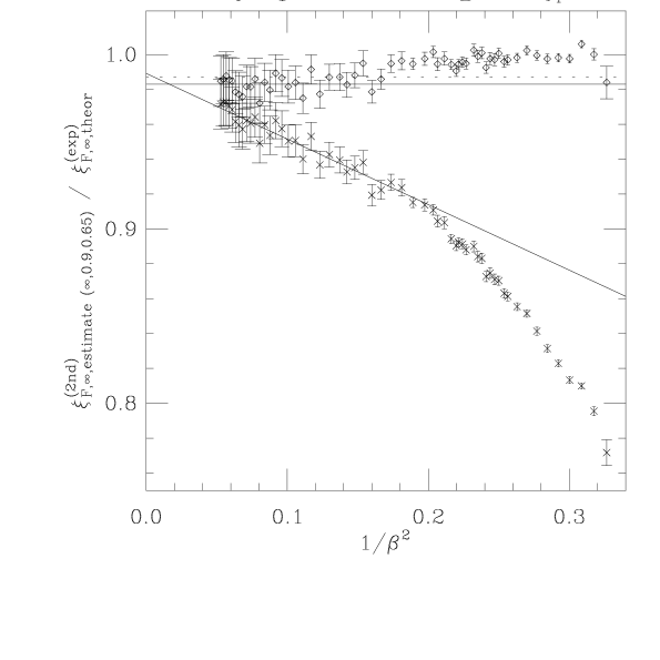
Figure 17: (a) $\xi^{(2nd)}_{F,\infty,estimate\,(\infty,0.90,0.65)}/\xi^{(exp)}_{F,\infty,theor}$ versus $\beta$. Error bars are one standard deviation (statistical error only). There are four versions of $\xi^{(exp)}_{F,\infty,theor}$: standard perturbation theory in $1/\beta$ gives points $+$ (2-loop) and $\times$ (3-loop); “improved” perturbation theory in $1-E$ gives points $\Box$ (2-loop) and $\Diamond$ (3-loop). Dotted line is the Monte Carlo prediction $\widetilde{C}_{\xi_{F}^{(2nd)}}/\widetilde{C}_{\xi_{F}^{(exp)}}=0.987\pm 0.002$ [67]. (b) Same ratio plotted versus $1/\beta^{2}$. The lower solid line is the fit $\kappa_{0}+\kappa_{2}/\beta^{2}$ to the standard 3-loop estimates ($\times$) for $\beta\geq 2.60$. The upper solid line is the constant fit $\kappa^{\prime}_{0}$ to the “improved” 3-loop estimates ($\Diamond$) for $\beta\geq 2.60$. Dashed line is the Monte Carlo prediction $\widetilde{C}_{\xi_{F}^{(2nd)}}/\widetilde{C}_{\xi_{F}^{(exp)}}=0.987\pm 0.002$ [67].

Let us recall that perturbation theory (3.3)/(3.9) combined with the nonperturbative (BNNW) prefactor (3.16) give a quantitative prediction for the exponential correlation length $\xi_{F}^{(exp)}$ [cf. (3.17a,c)]. The factor $\xi_{F}^{(2nd)}/\xi_{F}^{(exp)}$ is unknown, but a high-precision Monte Carlo study of the $SU(3)$ chiral model yields the value $0.987\pm 0.002$ [67]. We shall therefore plot $\xi_{F}^{(2nd)}(\beta)$ divided by $\xi_{F,\hbox{\scriptsize BNNW},k-loop}^{(exp)}(\beta)$ for $k=2,3$, and look for convergence as $\beta\to\infty$ to a value $\approx 0.987$. The results are shown in Figure 17(a) (points $+$ and $\times$). The discrepancy from two-loop asymptotic scaling, which is $\approx 20\%$ at $\beta=2.0$ ($\xi_{F,\infty}\approx 25$), decreases to 5–6% at $\beta=4.35$ ($\xi_{F,\infty}\approx 3.7\times 10^{5}$). The discrepancy from three-loop asymptotic scaling, which is $\approx 12\%$ at $\beta=2.0$, decreases to 2–3% at $\beta=4.35$. Furthermore, if we fit $\xi_{F}^{(2nd)}/\xi_{F,{\hbox{\scriptsize BNNW}},3-loop}^{(exp)}=\kappa_{0}+\kappa_{2}\beta^{-2}$, a good fit is obtained if we restrict attention to the points with $\beta\geq 2.60$ ($\xi_{F,\infty}\mathrel{\hbox to0.0pt{\lower 3.0pt\hbox{$\mathchar 536\relax$}\hss}\raise 2.0pt\hbox{$\mathchar 318\relax$}}300$), and we obtain the estimates

$$\widetilde{C}_{\xi_{F}^{(2nd)}}/\widetilde{C}_{\xi_{F}^{(exp)}}\equiv\kappa_{0}&=0.989\pm 0.007\\ a_{2}\equiv\kappa_{2}/\kappa_{0}=-0.38\pm 0.06{}$$ (5.63)

[see Figure 17(b), points $\times$]. Of course, this estimate of $a_{2}$ should not be taken too seriously, as we have neglected corrections of order $\beta^{-3}$ and higher; it is in any case of the same order of magnitude as the known value $a_{1}=-0.164$. Moreover, the error bar on $\kappa_{0}$ is probably significantly underestimated, because in this fit we have ignored the correlations between the estimated values $\xi_{F,\infty}^{(2nd)}$ at different $\beta$ [which arise from errors of type (iii)]. Still, the agreement with the predicted value 0.987 is remarkable.

We can also try “improved expansion parameters” (see Section 3.3). For example, we can use $x_{F}\equiv 1-E_{F}$ as a substitute for $\beta$, and compare to the prediction (3.19)/(3.20) for $\xi_{F}^{(exp)}$ as a function of $1-E_{F}$. For $E_{F}$ we use the value measured on the largest lattice (which is usually $L=128$); the statistical errors and finite-size corrections on $E_{F}$ are less than $5\times 10^{-4}$, and they induce an error less than $0.85\%$ on the predicted $\xi_{F,\infty}$ (less than 0.55% for $\beta\geq 2.2$). In Figure 17(a) (points $\Box$ and $\Diamond$) we show $\xi_{F}^{(2nd)}$ divided by the two-loop and three-loop perturbative predictions (3.19)/(3.20) for $\xi_{F}^{(exp)}$. The data agree with the two-loop prediction to within better than 5% for $\beta\geq 2.10$ ($\xi_{F,\infty}\mathrel{\hbox to0.0pt{\lower 3.0pt\hbox{$\mathchar 536\relax$}\hss}\raise 2.0pt\hbox{$\mathchar 318\relax$}}40$). The agreement with the three-loop prediction is excellent: the discrepancy is $\mathrel{\hbox to0.0pt{\lower 3.0pt\hbox{$\mathchar 536\relax$}\hss}\raise 2.0pt\hbox{$\mathchar 316\relax$}}1$–2% for $\beta\geq 1.75$ ($\xi_{F,\infty}\mathrel{\hbox to0.0pt{\lower 3.0pt\hbox{$\mathchar 536\relax$}\hss}\raise 2.0pt\hbox{$\mathchar 318\relax$}}8$). Furthermore, the “improved” 3-loop prediction is extremely flat, and to a constant $\kappa^{\prime}_{0}$ if we restrict attention to the points with $\beta\geq 2.60$ ($\xi_{F,\infty}\mathrel{\hbox to0.0pt{\lower 3.0pt\hbox{$\mathchar 536\relax$}\hss}\raise 2.0pt\hbox{$\mathchar 318\relax$}}300$), yielding the estimate

$$\widetilde{C}_{\xi_{F}^{(2nd)}}/\widetilde{C}_{\xi_{F}^{(exp)}}\equiv\kappa^{\prime}_{0}=0.983\pm 0.002$$ (5.64)

[see Figure 17(b), points $\Diamond$].

In conclusion, the three-loop perturbative prediction in the bare parameter agrees with the Monte Carlo data to within about 2–3% for $\beta\geq 4.05$ ($\xi_{F,\infty}\mathrel{\hbox to0.0pt{\lower 3.0pt\hbox{$\mathchar 536\relax$}\hss}\raise 2.0pt\hbox{$\mathchar 318\relax$}}10^{5}$), and three-loop “improved” perturbative prediction is even better ($<1$%). Furthermore, both the bare parameter and the “improved” perturbative predictions are extremely flat for $\beta\geq 3.15$ and $\beta\geq 2.35$, respectively. A good compromise for the limiting value would be

$$\widetilde{C}_{\xi_{F}^{(2nd)}}/\widetilde{C}_{\xi_{F}^{(exp)}}=0.985\pm 0.007\;,$$ (5.65)

which is in excellent agreement with the Rossi-Vicari prediction $0.987\pm 0.002$ [67].

5.3.4 Fundamental Sector: Susceptibility

For the susceptibility $\chi_{F}$ we proceed in two different ways: using either $\chi_{F}$ directly or else using the ratio $\chi_{F}/{\xi_{F}^{(2nd)}}^{2}$. The advantage of the latter approach is that one additional term of perturbation theory is available.

In Figure 18(a) we plot $\chi_{F,\infty,estimate\,(\infty,\infty,0.80)}$ divided by the theoretical prediction (3.4)/(3.10) with the prefactor $\widetilde{C}_{\chi_{F}}$ omitted; the $\beta\rightarrow\infty$ limit of this curve thus gives an estimate of $\widetilde{C}_{\chi_{F}}$. Here we have two-loop and three-loop predictions (points $+$, $\times$) as well as “improved” two-loop and three-loop predictions ($\Box$, $\Diamond$). The estimates from two-loop and three-loop standard perturbation theory (which are virtually identical since $b_{1}\approx-0.023$ is so small) are strongly rising for $\beta\mathrel{\hbox to0.0pt{\lower 3.0pt\hbox{$\mathchar 536\relax$}\hss}\raise 2.0pt\hbox{$\mathchar 316\relax$}}2.4$ and weakly rising thereafter. If we fit $\chi_{F}/(\chi_{F,3-loop}\hbox{ without the prefactor }$ $\widetilde{C}_{\chi_{F}})=\kappa_{0}+\kappa_{2}\beta^{-2}$, a good fit is obtained if we restrict attention to the points with $\beta\geq 2.65$ ($\xi_{F,\infty}\mathrel{\hbox to0.0pt{\lower 3.0pt\hbox{$\mathchar 536\relax$}\hss}\raise 2.0pt\hbox{$\mathchar 318\relax$}}360$), and we obtain the estimates

$$\widetilde{C}_{\chi_{F}}\equiv\kappa_{0}&=16.75\pm 0.31{}\\ b_{2}\equiv\kappa_{2}/\kappa_{0}=-0.72\pm 0.12$$ (5.66)

[see Figure 18(b), points $\times$]. The estimates from “improved” perturbation theory are rather flatter, particularly the three-loop one which is virtually constant for $\beta\mathrel{\hbox to0.0pt{\lower 3.0pt\hbox{$\mathchar 536\relax$}\hss}\raise 2.0pt\hbox{$\mathchar 318\relax$}}2.45$ ($\xi_{F,\infty}\mathrel{\hbox to0.0pt{\lower 3.0pt\hbox{$\mathchar 536\relax$}\hss}\raise 2.0pt\hbox{$\mathchar 318\relax$}}160$). The “improved” 3-loop values can be fit well to a constant $\kappa^{\prime}_{0}$ if we restrict attention to $\beta\geq 2.55$ ($\xi_{F,\infty}\mathrel{\hbox to0.0pt{\lower 3.0pt\hbox{$\mathchar 536\relax$}\hss}\raise 2.0pt\hbox{$\mathchar 318\relax$}}240$), and we obtain the estimate

$$\widetilde{C}_{\chi_{F}}\equiv\kappa^{\prime}_{0}=16.30\pm 0.07$$ (5.67)

[see Figure 18(b), points $\Diamond$]. This estimate is slightly lower than (LABEL:C_chi_F:1), but consistent with it.

Similarly, we could plot $(\chi_{F}/{\xi_{F}^{(2nd)}}^{2})_{\infty,estimate\,(\infty,\infty,\infty)}$ divided by the theoretical prediction (3.7)/(3.11)/(3.12) with the prefactors $\widetilde{C}_{\chi_{F}}$ and $\widetilde{C}_{\xi_{F}^{(2nd)}}$ omitted; the $\beta\rightarrow\infty$ limit of this curve would thus give an estimate of $\widetilde{C}_{\chi_{F}}/(\widetilde{C}_{\xi_{F}^{(2nd)}})^{2}$. However, in order to make the vertical scale of this graph more directly comparable to that of Figure 18, we have multiplied the quantity being plotted by $(\widetilde{C}^{({\hbox{\scriptsize BNNW}})}_{\xi_{F}^{(exp)}})^{2}$. Note that this does not in any way alter the logic of the analysis, as $\widetilde{C}^{({\hbox{\scriptsize BNNW}})}_{\xi_{F}^{(exp)}}$ is an explicit number defined in (3.16). The resulting curve is plotted in Figure 19(a); its $\beta\rightarrow\infty$ limit gives an estimate of $\widetilde{C}_{\chi_{F}}\times(\widetilde{C}_{\xi_{F}^{(2nd)}}/\widetilde{C}^{({\hbox{\scriptsize BNNW}})}_{\xi_{F}^{(exp)}})^{-2}$. In this case we have two-loop, three-loop and four-loop predictions ($+$, $\times$, +––$\tiny\vdash$$\tiny\dashv$) as well as “improved” two-loop, three-loop and four-loop predictions ($\Box$, $\Diamond$, $\bigcirc$). To convert this number to an estimate for $\widetilde{C}_{\chi_{F}}$ itself, we need to multiply by

$$\left({\widetilde{C}_{\xi_{F}^{(2nd)}}\over\widetilde{C}^{({\hbox{\scriptsize BNNW}})}_{\xi_{F}^{(exp)}}}\right)^{\!2}\,=\,\left({\widetilde{C}_{\xi_{F}^{(2nd)}}\over\widetilde{C}_{\xi_{F}^{(exp)}}}\right)^{\!2}\left({\widetilde{C}_{\xi_{F}^{(exp)}}\over\widetilde{C}_{\xi_{F}^{(exp)}}^{({\hbox{\scriptsize BNNW}})}}\right)^{\!2}\;.$$ (5.68)

The first factor on the right side has been estimated by Monte Carlo simulations [67], yielding $0.987^{2}=0.974$; moreover, our data for $\xi_{F}^{(2nd)}$ itself (Figure 17) are consistent with this prediction. The second factor on the right side is presumably equal to 1 (exactly). So we can take the factor (5.68) to be $\approx 0.974$. The estimates from the three-loop standard perturbation theory are rapidly decreasing for $\beta\mathrel{\hbox to0.0pt{\lower 3.0pt\hbox{$\mathchar 536\relax$}\hss}\raise 2.0pt\hbox{$\mathchar 316\relax$}}3.2$ and slowly decreasing thereafter; if we fit them to $\kappa_{0}+\kappa_{2}\beta^{-2}$, a good fit is obtained if we restrict attention to $\beta\geq 2.30$ ($\xi_{F,\infty}\mathrel{\hbox to0.0pt{\lower 3.0pt\hbox{$\mathchar 536\relax$}\hss}\raise 2.0pt\hbox{$\mathchar 318\relax$}}85$), and we obtain the estimates

$$\widetilde{C}_{\chi_{F}}\left({\widetilde{C}_{\xi_{F}^{(2nd)}}\over\widetilde{C}^{({\hbox{\scriptsize BNNW}})}_{\xi_{F}^{(exp)}}}\right)^{\!-2}\equiv\kappa_{0}&=16.61\pm 0.04\\ c_{2}\equiv\kappa_{2}/\kappa_{0}=0.34\pm 0.02{}$$ (5.69)

and hence

$$\widetilde{C}_{\chi_{F}}=16.17\pm 0.04\;.$$ (5.70)

The estimate (LABEL:c2:chi_F_stuff) is in excellent agreement with the known value $c_{2}=0.306$. If we now fit the standard four-loop values to $\kappa_{0}+\kappa_{3}\beta^{-3}$, we have a good fit for $\beta\geq 2.60$ ($\xi_{F,\infty}\mathrel{\hbox to0.0pt{\lower 3.0pt\hbox{$\mathchar 536\relax$}\hss}\raise 2.0pt\hbox{$\mathchar 318\relax$}}300$), and we obtain the estimates

$$\widetilde{C}_{\chi_{F}}\left({\widetilde{C}_{\xi_{F}^{(2nd)}}\over\widetilde{C}^{({\hbox{\scriptsize BNNW}})}_{\xi_{F}^{(exp)}}}\right)^{\!-2}\equiv\kappa_{0}&=16.74\pm 0.04\\ c_{3}\equiv\kappa_{3}/\kappa_{0}=0.19\pm 0.07$$ (5.71)

[see Figure 19(b), points +––$\tiny\vdash$$\tiny\dashv$], and hence

$$\widetilde{C}_{\chi_{F}}=16.30\pm 0.04\;.$$ (5.72)

The estimates from “improved” perturbation theory are much flatter, particularly the four-loop one which is virtually constant for $\beta\mathrel{\hbox to0.0pt{\lower 3.0pt\hbox{$\mathchar 536\relax$}\hss}\raise 2.0pt\hbox{$\mathchar 318\relax$}}2.3$. If we fit the “improved” three-loop values to $\kappa^{\prime}_{0}+\kappa^{\prime}_{2}\beta^{-2}$ for $\beta\geq 2.25$ ($\xi_{F,\infty}\mathrel{\hbox to0.0pt{\lower 3.0pt\hbox{$\mathchar 536\relax$}\hss}\raise 2.0pt\hbox{$\mathchar 318\relax$}}70$), we get

$$\widetilde{C}_{\chi_{F}}\left({\widetilde{C}_{\xi_{F}^{(2nd)}}\over\widetilde{C}^{({\hbox{\scriptsize BNNW}})}_{\xi_{F}^{(exp)}}}\right)^{\!-2}\equiv\kappa^{\prime}_{0}&=16.75\pm 0.04\\ c^{(imp)}_{2}\equiv\kappa^{\prime}_{2}/\kappa^{\prime}_{0}=-0.3\pm 0.2{}$$ (5.73)

and hence

$$\widetilde{C}_{\chi_{F}}=16.31\pm 0.04\;.$$ (5.74)

The estimate (LABEL:c2_imp:chi_F_stuff) suggests that $c^{(imp)}_{2}$ is very close to zero, consistent with the known value $c^{(imp)}_{2}=0.0010$. If we now fit the “improved” four-loop values to $\kappa^{\prime}_{0}+\kappa^{\prime}_{3}\beta^{-3}$, we have a good fit for $\beta\geq 2.075$ ($\xi_{F,\infty}\mathrel{\hbox to0.0pt{\lower 3.0pt\hbox{$\mathchar 536\relax$}\hss}\raise 2.0pt\hbox{$\mathchar 318\relax$}}34$), and we obtain the estimates

$$\widetilde{C}_{\chi_{F}}\left({\widetilde{C}_{\xi_{F}^{(2nd)}}\over\widetilde{C}^{({\hbox{\scriptsize BNNW}})}_{\xi_{F}^{(exp)}}}\right)^{\!-2}\equiv\kappa^{\prime}_{0}&=16.85\pm 0.03\\ c_{3}^{(imp)}\equiv\kappa^{\prime}_{3}/\kappa^{\prime}_{0}=0.10\pm 0.02$$ (5.75)

[see Figure 19(b), points $\bigcirc$], and hence

$$\widetilde{C}_{\chi_{F}}=16.41\pm 0.03\;.$$ (5.76)

In summary, all methods yield consistent results, but the ones based on $\chi_{F}/{\xi_{F}^{(2nd)}}^{2}$ show an earlier convergence to the limiting constant. Therefore, a reasonable compromise would be

$$\widetilde{C}_{\chi_{F}}\approx 16.35\pm 0.20\;.$$ (5.77)

5.3.5 Adjoint Sector: Correlation Length

Now let us look at the adjoint sector. We start with the correlation length $\xi_{A}^{(2nd)}$, which we can compare with the two-loop and three-loop perturbative predictions (3.3)/(3.9). Combined with the nonperturbative (BNNW) prefactor (3.15)/(3.16), these formulae give a quantitative prediction for the exponential correlation length $\xi_{A}^{(exp)}$ [cf. (3.17b,d)]. By plotting $\xi_{A}^{(2nd)}/\xi^{(exp)}_{A,{\hbox{\scriptsize BNNW}},k-loop}$ for $k=2,3$, we can test asymptotic scaling and estimate the universal nonperturbative ratio $\widetilde{C}_{\xi_{A}^{(2nd)}}/\widetilde{C}_{\xi^{(exp)}_{A}}$.

In Figure 20(a) we plot $\xi_{A,\infty,estimate\,(\infty,\infty,\infty)}^{(2nd)}/\xi^{(exp)}_{A,{\hbox{\scriptsize BNNW}},k-loop}$ versus $\beta$ (points $+$ and $\times$). We see that the behavior is similar to that observed in the fundamental channel (Figure 17); this is inevitable since the ratio $\xi_{F,\infty}^{(2nd)}/\xi_{A,\infty}^{(2nd)}$ is empirically close to constant ($\approx 2.80$) in this region. However, in the adjoint channel the estimates show strange (and presumably spurious) pseudo-periodic oscillations; we do not understand their cause, but they presumably arise from some quirks in the extrapolation to infinite volume. Furthermore, these values present an apparent change of slope at $\beta\approx 3.15$, suggesting a positive coefficient $a_{2}$, which is in total disagreement with the result (LABEL:a2:fit) predicted by fitting the fundamental-sector quantities. Perhaps we have grossly underestimated the systematic errors in the extrapolation to infinite volume, especially for for $\beta\mathrel{\hbox to0.0pt{\lower 3.0pt\hbox{$\mathchar 536\relax$}\hss}\raise 2.0pt\hbox{$\mathchar 318\relax$}}3.15$. The estimate of $\xi_{A}^{(2nd)}/\xi_{A,{\hbox{\scriptsize BNNW}},3-loop}^{(exp)}$ will depend whether or not we trust our extrapolation for $\beta\mathrel{\hbox to0.0pt{\lower 3.0pt\hbox{$\mathchar 536\relax$}\hss}\raise 2.0pt\hbox{$\mathchar 318\relax$}}3.15$. If we do not trust it, we may discard all those points with $\beta\mathrel{\hbox to0.0pt{\lower 3.0pt\hbox{$\mathchar 536\relax$}\hss}\raise 2.0pt\hbox{$\mathchar 318\relax$}}3.15$ and fit $\xi_{A}^{(2nd)}/\xi_{A,{\hbox{\scriptsize BNNW}},3-loop}^{(exp)}=\kappa_{0}+\kappa_{2}\beta^{-2}$. A good fit is obtained for $3.15\geq\beta\geq 2.40$ ($1.1\times 10^{3}\mathrel{\hbox to0.0pt{\lower 3.0pt\hbox{$\mathchar 536\relax$}\hss}\raise 2.0pt\hbox{$\mathchar 318\relax$}}\xi_{F}\mathrel{\hbox to0.0pt{\lower 3.0pt\hbox{$\mathchar 536\relax$}\hss}\raise 2.0pt\hbox{$\mathchar 318\relax$}}130$), and we obtain the estimates

$$\widetilde{C}_{\xi_{A}^{(2nd)}}/\widetilde{C}_{\xi_{A}^{(exp)}}\equiv\kappa_{0}&=0.71\pm 0.02{}\\ a_{2}\equiv\kappa_{2}/\kappa_{0}=-0.43\pm 0.10$$ (5.78)

[see Figure 18(b), points $\times$]. It is interesting to note the rough agreement between this prediction of $a_{2}$ and (LABEL:a2:fit). On the other hand, if we trust our extrapolation of $\xi_{A,\infty}$, we try a similar fit including all values of $\beta$. We obtain a good fit if we restrict attention to the points with $\beta\geq 3.15$ ($\xi_{F}\mathrel{\hbox to0.0pt{\lower 3.0pt\hbox{$\mathchar 536\relax$}\hss}\raise 2.0pt\hbox{$\mathchar 318\relax$}}2.7\times 10^{3}$), yielding the estimates

$$\widetilde{C}_{\xi_{A}^{(2nd)}}/\widetilde{C}_{\xi_{A}^{(exp)}}\equiv\kappa_{0}&=0.63\pm 0.02\\ a_{2}\equiv\kappa_{2}/\kappa_{0}=0.8\pm 0.4$$ (5.79)

The total disagreement between this prediction of $a_{2}$ and (LABEL:a2:fit) seems to indicate that (5.78) is more trustworthy.

The “improved” three-loop estimates of course show the same pseudo-periodic oscillations. If we fit $\xi_{A}^{(2nd)}/\xi_{A,{\hbox{\scriptsize BNNW}},3-loop}^{(exp)}=\kappa^{\prime}_{0}+\kappa^{\prime}_{2}\beta^{-2}$, a good fit is obtained for $\beta\geq 2.925$ ($\xi_{F}\mathrel{\hbox to0.0pt{\lower 3.0pt\hbox{$\mathchar 536\relax$}\hss}\raise 2.0pt\hbox{$\mathchar 318\relax$}}1.1\times 10^{3}$), and we obtain the estimates

$$\widetilde{C}_{\xi_{A}^{(2nd)}}/\widetilde{C}_{\xi_{A}^{(exp)}}\equiv\kappa^{\prime}_{0}&=0.65\pm 0.02{}\\ a^{(imp)}_{2}\equiv\kappa^{\prime}_{2}/\kappa^{\prime}_{0}=0.8\pm 0.3$$ (5.80)

[see Figure 18(b), points $\Diamond$]. However, this is not consistent with the estimate $a_{2}^{(imp)}=-0.04\pm 0.05$ obtained from the fundamental sector (see footnote 32).

These estimates can be compared with the combination

$${\widetilde{C}_{\xi_{A}^{(2nd)}}\over\widetilde{C}_{\xi^{(exp)}_{A}}}\,=\,\left({\widetilde{C}_{\xi_{A}^{(2nd)}}\over\widetilde{C}_{\xi_{F}^{(2nd)}}}\right)\,\left({\widetilde{C}_{\xi_{F}^{(2nd)}}\over\widetilde{C}_{\xi_{F}^{(exp)}}}\right)\,\left({\widetilde{C}_{\xi_{F}^{(exp)}}\over\widetilde{C}_{\xi_{A}^{(exp)}}}\right)\,$$ (5.81)

of our previous estimates. Our estimate of the first term of the right side is $1/(2.80\pm 0.05)=0.357\pm 0.006$ [see (5.45)]; Monte Carlo simulations [67] predict that the second term of the right side is $0.987\pm 0.002$; and the theoretical prediction for the third term of the right side is exactly 2 [see (3.15)]. This approach yields

$${{\widetilde{C}_{\xi_{A}^{(2nd)}}}\over\widetilde{C}_{{\xi^{(exp)}_{A,3-loop}}}}=0.70\pm 0.01\;.$$ (5.82)

Let us recall that this approach suffers from various difficulties in the estimation of $\xi_{A}^{(2nd)}/\xi_{F}^{(2nd)}$ (see Section 5.2.2); but, in spite of that, the result (5.82) is consistent with (LABEL:C_xiA:1), and marginally consistent with (LABEL:C_xiA:2). A reasonable compromise would be to take

$${\widetilde{C}_{\xi_{A}^{(2nd)}}\over\widetilde{C}_{\xi^{(exp)}_{A}}}\approx 0.69\pm 0.04\;.$$ (5.83)

5.3.6 Adjoint Sector: Susceptibility

The story for $\chi_{A}$ is similar to that of $\chi_{F}$: we can either use $\chi_{A}$ directly or else use the ratio $\chi_{A}/{\xi_{A}^{(2nd)}}^{2}$.

In Figure 21(a) we plot $\chi_{A,\infty,estimate\,(\infty,\infty,0.90)}$ divided by the theoretical prediction (3.5)/(3.13) with the prefactor $\widetilde{C}_{\chi_{A}}$ omitted; the $\beta\rightarrow\infty$ limit of this curve thus an estimate of $\widetilde{C}_{\chi_{A}}$. Here we have two-loop and three-loop predictions from standard perturbation theory (points $+$, $\times$) as well as “improved” two-loop and three-loop predictions ($\Box$, $\Diamond$). At each order (two-loop or three-loop), the standard and the “improved” estimates are virtually identical for $\beta\mathrel{\hbox to0.0pt{\lower 3.0pt\hbox{$\mathchar 536\relax$}\hss}\raise 2.0pt\hbox{$\mathchar 318\relax$}}3$; but for $\beta\mathrel{\hbox to0.0pt{\lower 3.0pt\hbox{$\mathchar 536\relax$}\hss}\raise 2.0pt\hbox{$\mathchar 316\relax$}}3$ the standard estimates are much flatter (in marked contrast to what is observed for $\xi_{F}$, $\chi_{F}$ and $\xi_{A}$: see Figures 17–20). This casts some doubts on whether the “improved” perturbation theory is always an improvement! If we fit the “standard” 3-loop perturbation values $\chi_{A}/(\chi_{A,3-loop}\hbox{ without the prefactor }$ $\widetilde{C}_{\chi_{A}})=\kappa_{0}+\kappa_{2}\beta^{-2}$, a good fit is obtained if we restrict attention to the points with $\beta\geq 2.25$ ($\xi_{F,\infty}\mathrel{\hbox to0.0pt{\lower 3.0pt\hbox{$\mathchar 536\relax$}\hss}\raise 2.0pt\hbox{$\mathchar 318\relax$}}70$), and we obtain the estimates

$$\widetilde{C}_{\chi_{A}}\equiv\kappa_{0}&=196\pm 2{}\\ d_{2}\equiv\kappa_{2}/\kappa_{0}=0.14\pm 0.50$$ (5.84)

[see Figure 21(b), points $\times$]. Similarly, if we fit the “improved” 3-loop perturbation values $\chi_{A}/(\chi_{A,3-loop}\hbox{ without the prefactor }\widetilde{C}_{\chi_{A}})=\kappa^{\prime}_{0}+\kappa^{\prime}_{2}\beta^{-2}$, a good fit is obtained for $\beta\geq 2.55$ ($\xi_{F,\infty}\mathrel{\hbox to0.0pt{\lower 3.0pt\hbox{$\mathchar 536\relax$}\hss}\raise 2.0pt\hbox{$\mathchar 318\relax$}}110$), and we get

$$\widetilde{C}_{\chi_{A}}\equiv\kappa^{\prime}_{0}&=191\pm 3{}\\ d^{(imp)}_{2}\equiv\kappa^{\prime}_{2}/\kappa^{\prime}_{0}=0.53\pm 0.12$$ (5.85)

[see Figure 21(b), points $\Diamond$].

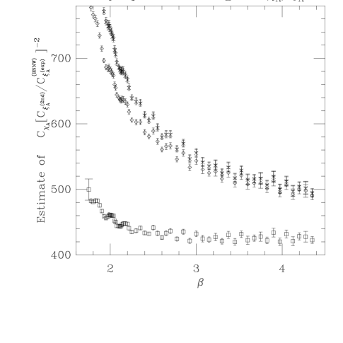
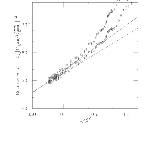
Figure 22: (a) $[(\chi_{A}/\xi^{(2nd)^{2}}_{A})_{\infty,estimate(\infty,\infty,\infty)}]\,\times\,[\widetilde{C}^{{\hbox{\scriptsize BNNW}}}_{\xi^{(exp)}_{A}}]^{2}\,/$ $[(\chi_{A}/\xi^{(2nd)^{2}}_{A})_{\infty,theor}\hbox{ without prefactors }\widetilde{C}_{\chi_{A}}\hbox{ and }\widetilde{C}_{\xi^{(2nd)}_{A}}]$ versus $\beta$. Error bars are one standard deviation (statistical error only). There are four versions of $(\chi_{A}/\xi_{A}^{2})_{\infty,theor}$: standard perturbation theory in $1/\beta$ gives points $+$ (2-loop) and $\times$ (3-loop); “improved” perturbation theory in $1-E$ gives points $\Box$ (2-loop) and $\Diamond$ (3-loop). (b) Same quantity plotted versus $1/\beta^{2}$. The steeper solid line is the fit $\kappa_{0}+\kappa_{2}/\beta^{2}$ to the standard 3-loop estimates ($\times$) for $\beta\geq 3.075$. The flatter solid line is the fit $\kappa^{\prime}_{0}+\kappa^{\prime}_{2}/\beta^{2}$ to the “improved” 3-loop estimates ($\Diamond$) for $\beta\geq 3.075$.

Similarly, we could plot $(\chi_{A}/{\xi_{A}^{(2nd)}}^{2})_{\infty,estimate\,(\infty,\infty,\infty)}$ divided by the theoretical prediction (3.8)/(3.14) with the prefactors $\widetilde{C}_{\chi_{A}}$ and $\widetilde{C}_{\xi_{A}^{(2nd)}}$ omitted; the $\beta\rightarrow\infty$ limit of this curve would thus give an estimate of $\widetilde{C}_{\chi_{A}}/(\widetilde{C}_{\xi_{A}^{(2nd)}})^{2}$. However, in order to make the vertical scale of this graph more directly comparable to that of Figure 21(a), we have multiplied the quantity being plotted by $(\widetilde{C}^{({\hbox{\scriptsize BNNW}})}_{\xi_{A}^{(exp)}})^{2}$. Note that this does not in any way alter the logic of the analysis, as $\widetilde{C}^{({\hbox{\scriptsize BNNW}})}_{\xi_{A}^{(exp)}}$ is an explicit number obtained from (3.15)/(3.16). The resulting curve is plotted in Figure 22(a); its $\beta\rightarrow\infty$ limit gives an estimate of $\widetilde{C}_{\chi_{A}}\,(\widetilde{C}^{({\hbox{\scriptsize BNNW}})}_{\xi_{A}^{(exp)}}/\widetilde{C}_{\xi_{A}^{(2nd)}})^{2}$. In this case we just have two-loop and three-loop predictions ($+$, $\times$) as well as “improved” two-loop and three-loop predictions ($\Box$, $\Diamond$). To convert this number to an estimate for $\widetilde{C}_{\chi_{A}}$ itself, we need to multiply by

$$\left({\widetilde{C}_{\xi_{A}^{(2nd)}}\over\widetilde{C}^{({\hbox{\scriptsize BNNW}})}_{\xi_{A}^{(exp)}}}\right)^{\!2}\approx(0.69\pm 0.04)^{2}=0.476\pm 0.055$$ (5.86)

[see (5.83)]. The estimates from two-loop and three-loop standard perturbation theory (which are virtually identical since $e_{1}\approx 0.0075$ is so small) are strongly decreasing for $\beta\mathrel{\hbox to0.0pt{\lower 3.0pt\hbox{$\mathchar 536\relax$}\hss}\raise 2.0pt\hbox{$\mathchar 316\relax$}}3.0$ and weakly decreasing thereafter. If we fit the 3-loop values to $\kappa_{0}+\kappa_{2}\beta^{-2}$, a good fit is obtained if we restrict attention to the points with $\beta\geq 3.075$ ($\xi_{F,\infty}\mathrel{\hbox to0.0pt{\lower 3.0pt\hbox{$\mathchar 536\relax$}\hss}\raise 2.0pt\hbox{$\mathchar 318\relax$}}2\times 10^{3}$), and we obtain the estimates

$$\widetilde{C}_{\chi_{A}}\left({\widetilde{C}_{\xi_{A}^{(2nd)}}\over\widetilde{C}^{({\hbox{\scriptsize BNNW}})}_{\xi_{A}^{(exp)}}}\right)^{\!-2}\equiv\kappa_{0}&=456\pm 8\\ e_{2}\equiv\kappa_{2}/\kappa_{0}=1.8\pm 0.3$$ (5.87)

and hence

$$\widetilde{C}_{\chi_{A}}=217\pm 16\;$$ (5.88)

[see Figure 22(b), points $\times$]. This estimate is in reasonable agreement with the previous predictions (LABEL:pred_chi_a_bare) and (LABEL:pred_chi_a_imp), but exhibits much larger uncertainties (in contrast to the situation observed for the fundamental susceptibility, where $\chi_{F}/\xi_{F}^{(2nd)}$ is better behaved than $\chi_{F}$). The estimates from “improved” three-loop perturbation theory are are virtually identical to those from three-loop standard perturbation theory. If we fit the “improved” three-loop estimates to $\kappa^{\prime}_{0}+\kappa^{\prime}_{2}\beta^{-2}$, a good fit is obtained for $\beta\geq 3.075$ ($\xi_{F,\infty}\mathrel{\hbox to0.0pt{\lower 3.0pt\hbox{$\mathchar 536\relax$}\hss}\raise 2.0pt\hbox{$\mathchar 318\relax$}}2\times 10^{3}$), and we obtain the estimates

$$\widetilde{C}_{\chi_{A}}\left({\widetilde{C}_{\xi_{A}^{(2nd)}}\over\widetilde{C}^{({\hbox{\scriptsize BNNW}})}_{\xi_{A}^{(exp)}}}\right)^{\!-2}\equiv\kappa^{\prime}_{0}&=459\pm 7\\ e^{(imp)}_{2}\equiv\kappa^{\prime}_{2}/\kappa^{\prime}_{0}=1.5\pm 0.3$$ (5.89)

and hence

$$\widetilde{C}_{\chi_{A}}=218\pm 15\;$$ (5.90)

[see Figure 22(b), points $\Diamond$].

All methods yield consistent results, but the ones based on $\chi_{A}$ alone show an earlier convergence to the limiting constant; furthermore, as they do not require information about the constant (5.86). Thus, a reasonable compromise would be

$$\widetilde{C}_{\chi_{A}}\approx 195\pm 20\;.$$ (5.91)

5.4 Discussion

Let us summarize our findings. First, we hope to have convinced the reader that the extrapolation method has allowed us to obtain the infinite-volume behavior of long-distance observables with reliable control over all systematic and statistical errors, using only lattices $L\leq 256$. For example, we obtain the infinite-volume correlation length $\xi_{F,\infty}^{(2nd)}$ to a statistical accuracy of order 0.5% (resp. 0.9%, 1.1%, 1.3%, 1.5%) when $\xi_{F,\infty}^{(2nd)}\approx 10^{2}$ (resp. $10^{3}$, $10^{4}$, $10^{5}$, $4\times 10^{5}$); and the systematic errors arising from corrections to scaling are of the same order or smaller. The situation is similar for $\chi_{F}$ and $\chi_{A}$. Only for $\xi_{A}^{(2nd)}$ and the two ratios $\chi_{\#}/(\xi_{\#}^{(2nd)})^{2}$ do we have severe worries about the possible remaining corrections to scaling; for these observables it would be useful to carry out simulations at larger $L$, so that our fits can be checked against alternative fits with larger $L_{min}$.

It is important to remark that the validity of these extrapolated data rests on the assumption that if finite-size-scaling (5.2) is found empirically to be satisfied (with a given function $F_{\cal O}$) for some range of $L$, say $L_{min}\leq L\leq L_{max}$, then it will also hold (with the same $F_{\cal O}$) for $L>L_{max}$. Now, we have found that the data for 16–$32\leq L\leq 128$ are in good agreement with rapid convergence as $L$ grows at fixed $x\equiv\xi_{F}^{(2nd)}(L)/L$ to a finite-size-scaling function $F_{\cal O}(x;s)$. It is then reasonable to assume that the limiting function empirically obtained for $L\leq 128$ is close to the true limiting function as $L\rightarrow\infty$, i.e. that the systematic errors are in fact as small as they seem empirically to be. Of course, it is possible that apparent convergence of $F_{\cal O}(x;s)$ for 16–$32\leq L\leq 128$ is misleading — i.e. a “false plateau” — and that for very large values of $L$ the convergence is to a very different function (or there is convergence at all). This caveat is not special to our work, but is inherent in any numerical work that attempts to evaluate a limit (here $L\to\infty$) by taking the relevant parameter almost to the limit (here $L$ large but finite). In particular, this caveat is inherent in all numerical (as well as experimental) work in the fields of critical phenomena and quantum field theory.

In any case, there is no evidence that this unfortunate situation occurs in our model. Indeed, what is remarkable in our model is the extreme weakness of the corrections to scaling: for example, for ${\cal O}=\xi_{F}^{(2nd)}$, even at $L=8$ the corrections to scaling are almost unobservable for $x\mathrel{\hbox to0.0pt{\lower 3.0pt\hbox{$\mathchar 536\relax$}\hss}\raise 2.0pt\hbox{$\mathchar 318\relax$}}0.8$. Even at smaller values of $x$, where the corrections to scaling are clearly visible, they are perfectly consistent with a behavior roughly of the form

$${{\cal O}(\beta,2L)\over{\cal O}(\beta,L)}\;=\;F_{\cal O}(x)\,+\,{1\over L^{2}}G_{\cal O}(x)\,+\,\ldots\;,$$ (5.92)

at least in the range $8\leq L\leq 128$ where we have data. If all hell breaks loose for larger $L$, we certainly see no hint of it at $L\leq 128$.

Our second principal observation is that the finite-size-scaling functions $F_{\cal O}$, as determined from our Monte Carlo data by the above analysis, agree well with the perturbative predictions for large $x$ [cf. (3.24)]. More precisely, we found good agreement for $x\mathrel{\hbox to0.0pt{\lower 3.0pt\hbox{$\mathchar 536\relax$}\hss}\raise 2.0pt\hbox{$\mathchar 318\relax$}}0.6$–0.9 (depending on the observable) up to the largest $x$ observed in our data ($x_{max}\approx 1.2$).

We would like to clarify the logic concerning this point, which has caused some controversy [80, 81]. There are two very different limits that can be taken in a two-dimensional $\sigma$-model:

• the finite-volume perturbative limit $\beta\to\infty$ at fixed $L<\infty$;

• the finite-size-scaling limit $\beta\to\infty$ and $L\to\infty$ such that the ratio $x\equiv\xi(\beta,L)/L$ is held fixed.

There is no doubt that conventional perturbation theory [cf. (B.4)] is valid in limit (a): it concerns, after all, a finite-dimensional integral. The deep question is how the remainder terms in this asymptotic expansion behave as a function of $L$; one wants in particular to know whether the perturbation theory derived from the study of limit (a) is also correct in the double limit obtained by first taking limit (b) and then taking $x\to\infty$ [cf. (B.6)]. The conventional wisdom says yes: indeed, this or a similar interchange of limits underlies the conventional derivations of asymptotic freedom (a point that unfortunately has not always been clearly acknowledged by advocates of the conventional wisdom). By contrast, Patrascioiu and Seiler [39, 40, 42] say no: they suspect that asymptotic freedom is false [41]. At present, no rigorous proof is available to settle this question one way or the other.

Patrascioiu and Seiler [80] have objected that our data in the large-$x$ region are essentially perturbative, in the sense that they are well reproduced by the finite-volume perturbation theory [limit (a)], whose validity is not in question. For this reason, they contend, we are implicitly assuming asymptotic scaling. Our reply is twofold:

On the one hand, it is not quite true that our data in the large-$x$ region are “essentially perturbative”: as noted in Section 5.3.2, our raw data ${\cal O}(\beta,L)$ deviate significantly from the finite-volume perturbation expansions (B.24). In the fundamental sector, the deviation $|S_{3}|$ between $\chi_{F}$ and second-order perturbation theory is less than 1.0% (resp. 0.3%) for $x\geq 0.6$ (resp. $x\geq 0.9$); while the deviation $|R_{2}|$ between $\xi_{F}^{(2nd)}$ and first-order perturbation theory is less than 9.8% (resp. 4.1%) for these same intervals of $x$. All these deviations are observed at $L=128$, which is the largest value of $L$ for which we have data in the specified intervals of $x$; rather smaller deviations are obtained at the same $x$ and smaller $L$. For example, for $L=8$ we have discrepancies of 1.1% (resp. 0.2%) for $\chi_{F}$, and 6.5% (resp. 2.2%) for $\xi_{F}^{(2nd)}$. For the adjoint sector, the agreement with perturbation theory is much worse: at $L=128$, for $\chi_{A}$ we have discrepancies as large as 17.3% (resp. 6.2%) for $x\geq 0.6$ (resp. $x\geq 0.9$), while for $\xi_{A}^{(2nd)}$ the discrepancies reach 12.2% (resp. 5.0%). At $L=8$ things are much better for $\chi_{A}$, with discrepancies reaching only 1.3% (resp. 0.3%); but for $\xi_{A}^{(2nd)}$ they still reach 8.7% (resp. 3.0%).

Thus, it is only for $\chi_{F}$ (and $\chi_{A}$ on small lattices) that our data are in any sense “essentially perturbative”; all the other observables show significant deviations from finite-volume perturbation theory, even on the smallest lattices. [To be sure, the agreement for $\xi_{F}^{(2nd)}$ and $\xi_{A}^{(2nd)}$ would probably be improved dramatically if the two-loop (order-$1/\beta^{2}$) correction were available to us.]

Secondly, and more importantly, we have always analyzed our data in the sense of limit (b): that is, at each fixed $x\equiv\xi_{F}^{(2nd)}(\beta,L)/L$, we have asked whether the ratios ${\cal O}(\beta,2L)/{\cal O}(\beta,L)$ have a good limit as $L\to\infty$, and if so we have attempted to evaluate this limit numerically as explained above. Thus, modulo the caveats discussed in the preceding paragraphs, we believe we have determined (within statistical errors) the true finite-size-scaling functions $F_{\cal O}$. There is no contradiction between Patrascioiu–Seiler’s observation and ours: the same point $(\beta,L)$ may well lie within the range of validity (to some given accuracy) of two distinct expansions. The fact that some of our data points at large $x$ are consistent with finite-volume perturbation theory [limit (a)] does not constitute evidence against their also being consistent with nonperturbative finite-size scaling [limit (b)]. For this reason, we disagree with Patrascioiu–Seiler’s claim [80] that our method has implicitly assumed asymptotic scaling. Quite the contrary: our data at $x\mathrel{\hbox to0.0pt{\lower 3.0pt\hbox{$\mathchar 536\relax$}\hss}\raise 2.0pt\hbox{$\mathchar 318\relax$}}0.6$–0.9, interpreted in the sense of limit (b), constitute a test of the key assumptions underlying the derivation of asymptotic scaling.

Finally, we have made in Sections 5.3.3–5.3.6 a direct test of asymptotic scaling for the various infinite-volume long-distance observables ${\cal O}_{\infty}(\beta)$. As noted in the Introduction, this test involves two distinct questions:

• Does the ratio between the extrapolated values and the $l$-loop asymptotic-freedom prediction,

  $$C_{\cal O}(\beta)\;\equiv\;{{\cal O}_{\infty}(\beta)\over e^{a\beta}\beta^{b}(1+k_{1}/\beta+\cdots+k_{l}/\beta^{l})}\;,$$ (5.93)

  converge to a constant in the limit $\beta\to\infty$, modulo corrections of order $1/\beta^{l+1}$?

• In the case of ${\cal O}=\xi_{F}^{(2nd)}$, does this constant equal the nonperturbative value predicted by the thermodynamic Bethe Ansatz [62] combined with the best Monte Carlo estimate [67] of $\xi_{F}^{(2nd)}/\xi_{F}^{(exp)}$?

Patrascioiu and Seiler [80] are right to point out that our affirmative answer to question (i) is in some sense a foregone conclusion: since our Monte Carlo data for $F_{\cal O}(x)$ at $x\mathrel{\hbox to0.0pt{\lower 3.0pt\hbox{$\mathchar 536\relax$}\hss}\raise 2.0pt\hbox{$\mathchar 318\relax$}}0.6$–0.9 do in fact agree reasonably well with the two-loop perturbative formula (3.24), and our data for ${\cal O}(\beta,L)$ also agree at least roughly with the fixed-$L$ perturbation expansion (B.24), it is then inevitable that our extrapolated values ${\cal O}_{\infty}(\beta)$ at the largest values of $\beta$ will be consistent with two-loop asymptotic scaling in the sense that ${\cal O}_{\infty}(\beta)/[e^{a\beta}\beta^{b}]$ will be roughly constant. Therefore, our observation in Sections 5.3.3–5.3.6 of asymptotic scaling in sense (i) contains no significant information beyond our observation in Section 5.2.1 that the finite-size-scaling functions $F_{\cal O}(x)$ agree with the perturbative predictions at $x\mathrel{\hbox to0.0pt{\lower 3.0pt\hbox{$\mathchar 536\relax$}\hss}\raise 2.0pt\hbox{$\mathchar 318\relax$}}0.6$–0.9; this latter observation already contains the essence of asymptotic scaling in sense (i). On the other hand, asymptotic scaling in sense (ii) is truly an additional observation: it is by no means inevitable that the observed constant value of $C_{\xi_{F}^{(2nd)}}(\beta)$ at large $\beta$ will agree with the thermodynamic Bethe Ansatz prediction to within a fraction of a percent, as we have found here (Section 5.3.3). It seems to us that this apparent coincidence is significant evidence in favor of the asymptotic-freedom picture.

We have found empirically that the “energy-improved” perturbative expansion usually exhibits asymptotic scaling (to a given accuracy) at lower values of $\beta$ than its bare-parameter counterpart. The exceptions to this behavior are the observables $\chi_{A}$, for which standard perturbation theory has an incredibly flat behavior and the “energy-improved” perturbation theory is less well behaved, and $\chi_{A}/\xi_{A}^{2}$, for which the two expansions exhibit nearly identical behavior. This generally good behavior of the “energy-improved” expansion confirms similar observations in other models, such as the $N$-vector models for $N=3,4,8$ [112, 76, 77, 78, 79, 11], the $CP^{N-1}$ $\sigma$-models for $N=2,4,10$ [123], the $SU(N)$ chiral models for $N=4,6,9,15,21,30$ [66, 67, 93], and the $SU(2)$ and $SU(3)$ lattice gauge theories [100, 124, 125, 126, 127]. What we lack is a good theoretical explanation of this empirically observed behavior (see Section 3.3). It is not clear to us whether “improved” perturbation theory can systematically be expected to reach asymptotic scaling faster than standard perturbation theory (except for some unusual cases in which standard perturbation theory has small high-order terms), or whether its apparent success is illusory.

6 Finite-Size-Scaling Analysis: Dynamic Quantities

Of all the observables we studied, the slowest mode (by far) is the squared fundamental magnetization ${\cal M}_{F}^{2}$: this quantity measures the relative rotations of the spins in different parts of the lattice, and is the prototypical $SU(N)$-invariant “long-wavelength observable”. The autocorrelation time $\tau_{int,{\cal M}_{F}^{2}}$ has the following qualitative behavior: as a function of $\beta$ it first rises to a peak and then falls; the location of this peak shifts towards $\beta=\infty$ as $L$ increases; and the height of this peak grows as $L$ increases. A similar but less pronounced peak is observed in $\tau_{int,{\cal M}_{A}^{2}}$. By contrast, the integrated autocorrelation times of the energies, $\tau_{int,\,{\cal E}_{F}}$ and $\tau_{int,\,{\cal E}_{A}}$, are much smaller and vary only weakly with $\beta$ and $L$. This is because the energies are primarily “short-wavelength observables”, and have only weak overlap with the modes responsible for critical slowing-down.

Let us now make these considerations quantitative, by applying finite-size scaling to the dynamic quantities $\tau_{int,{\cal M}_{F}^{2}}$ and $\tau_{int,{\cal M}_{A}^{2}}$. We use the Ansatz

$$\tau_{int,A}(\beta,L)\;\sim\;\xi(\beta,L)^{z_{int,A}}\,g_{A}\Bigl{(}\xi(\beta,L)/L\Bigr{)}$$ (6.1)

for $A={\cal M}_{F}^{2}$ and ${\cal M}_{A}^{2}$. Here $g_{A}$ is an unknown scaling function, and $g_{A}(0)=\lim_{x\downarrow 0}g_{A}(x)$ is supposed to be finite and nonzero. We determine $z_{int,A}$ by plotting $\tau_{int,A}/\xi_{F}(L)^{z_{int,A}}$ versus $\xi_{F}(L)/L$ and adjusting $z_{int,A}$ until the points fall as closely as possible onto a single curve (with priority to the larger $L$ values). We emphasize that the dynamic critical exponent $z_{int,A}$ is in general different from the exponent $z_{exp}$ associated with the exponential autocorrelation time $\tau_{exp}$ [1, 128, 4].

Using the procedure just described, we find

$$z_{int,{\cal M}_{F}^{2}}\;=\;0.45\pm 0.02$$ (6.2)

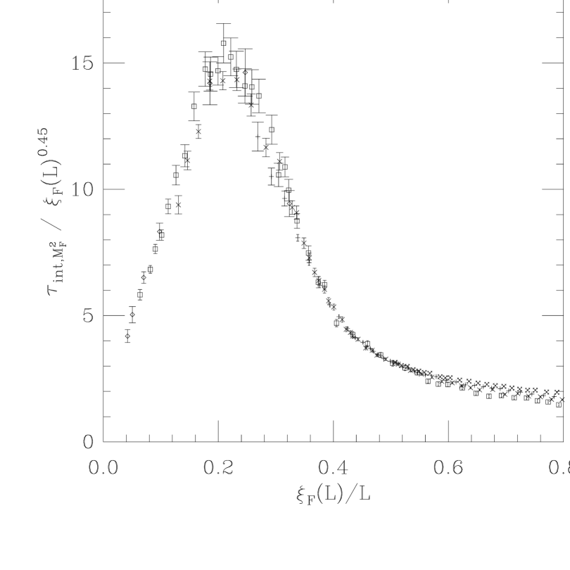
Figure 23: Dynamic finite-size-scaling plot of $\tau_{int,{\cal M}_{F}^{2}}/\xi_{F}^{(2nd)}(L)^{z_{int,{\cal M}_{F}^{2}}}$ versus $\xi_{F}^{(2nd)}(L)/L$. Symbols indicate $L=16$ ($\times$$\tiny\times$$\tiny\times$$\tiny\times$$\tiny\times$), 32 ($+$), 64 ($\times$), 128 ($\Box$) and 256 ($\Diamond$). Here $z_{int,{\cal M}_{F}^{2}}=0.45$. We have included in the plot only those points satisfying $\xi_{F}(L)\geq 8$.

(subjective 68% confidence limits). In Figure 23 we show the “best” finite-size-scaling plot. Note that the corrections to scaling are very weak: only the $L=16$ points clearly deviate from the asymptotic scaling curve; the $L=32$ and $L=64$ points show barely significant deviations.

It is worth noting that the finite-size effects on dynamic quantities are very strong at $\xi/L$ as small as 0.1 or even 0.05, whereas the finite-size effects on static quantities are negligible already when $\xi(L)/L\mathrel{\hbox to0.0pt{\lower 3.0pt\hbox{$\mathchar 536\relax$}\hss}\raise 2.0pt\hbox{$\mathchar 316\relax$}}0.15$: compare Figure 23 with Figure 1. Indeed, in Figure 23 it is far from clear what is the limiting value of the scaling function, $g_{{\cal M}_{F}^{2}}(0)=\lim_{x\downarrow 0}g_{{\cal M}_{F}^{2}}(x)$, and whether it is nonzero. This extremely strong dynamic finite-size effect (here a factor of order 5–10 for $\xi(L)/L$ between 0 and 0.2) seems to occur rather frequently in collective-mode Monte Carlo algorithms: see e.g. [8] for multi-grid in the two-dimensional 4-vector model, and [129] for the Swendsen-Wang-Wolff algorithm in the two-dimensional $RP^{N-1}$ models. We conclude that finite-size corrections to dynamic critical behavior can be surprisingly strong; therefore, serious studies of dynamic critical phenomena must include a finite-size-scaling analysis. It can be very misleading to assume that the finite-size corrections to dynamic quantities are small simply because $\xi/L$ is small, or because the finite-size corrections to static quantities are small.

We can also analyze the dynamic critical behavior for the adjoint sector. Proceeding as before, we obtain

$$z_{int,{\cal M}_{A}^{2}}\;=\;0.45\pm 0.03$$ (6.3)

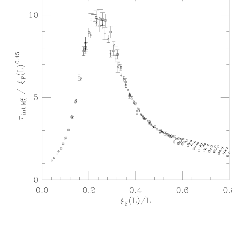
Figure 24: Dynamic finite-size-scaling plot of $\tau_{int,{\cal M}_{A}^{2}}/\xi_{F}^{(2nd)}(L)^{z_{int,{\cal M}_{A}^{2}}}$ versus $\xi_{F}^{(2nd)}(L)/L$. Symbols indicate $L=16$ ($\times$$\tiny\times$$\tiny\times$$\tiny\times$$\tiny\times$), 32 ($+$), 64 ($\times$), 128 ($\Box$) and 256 ($\Diamond$). Here $z_{int,{\cal M}_{A}^{2}}=0.45$. We have included in the plot only those points satisfying $\xi_{F}(L)\geq 8$.

(subjective 68% confidence limits). In Figure 24 we show the “best” finite-size-scaling plot. Note that both the magnitude and shape of the finite-size-scaling plot are similar for ${\cal M}_{F}^{2}$ and ${\cal M}_{A}^{2}$, although the details are slightly different. Note also that $z_{int,{\cal M}_{F}^{2}}$ and $z_{int,{\cal M}_{A}^{2}}$ are equal within error bars; this contrasts with the behavior observed in MGMC for the 3-vector model [11], in which the isotensor dynamic critical exponent $z_{int,{\cal M}_{T}^{2}}$ appears to be strictly smaller than the isovector exponent $z_{int,{\cal M}_{V}^{2}}$. More work will clearly be required to sort out what is going on here.

Appendix A Perturbation Theory for the Non-Derivative Irreducible Operators

In this section we will compute the perturbative (large-$\beta$) predictions for a general two-point correlation function

$$G_{r}(x;\beta)\;=\;{1\over d_{r}}\langle\chi_{r}(U_{0}U_{x}^{\dagger})\rangle$$ (A.1)

where the index $r$ labels an irreducible representation of $SU(N)$, $\chi_{r}$ is the associated character and $d_{r}$ its dimension. The perturbative expansion of $G_{r}(x;\beta)$ is obtained by setting

$$U_{x}\;=\;\exp(iA_{x})\qquad\hbox{with}\qquad A_{x}\;=\;A_{x}^{a}T^{a}$$ (A.2)

and then expanding in powers of $A$; here $T^{a}$ are the generators of the Lie algebra ${\hbox{\german su}(N)}$, normalized so that $\hbox{Tr}(T^{a}T^{b})={1\over 2}\delta^{ab}$, and $A_{x}^{a}$ are $N^{2}-1$ real fields. We must also take into account the contributions from the integration measure. A straightforward calculation [130, 38] shows that the Haar measure on $SU(N)$ is

$$dU_{x}&=dA_{x}\exp\left\{{1\over 2}\hbox{Tr}\log\left[2(1-\cos A^{a}_{x}T^{a}_{A})\over(A^{a}_{x}T^{a}_{A})^{2}\right]\right\}\\ =dA_{x}\exp\left[-{N\over 24}A^{a}_{x}A^{a}_{x}+O(A^{4})\right]\;,{}$$ (A.3)

where $(T^{a}_{A})_{bc}=-if^{abc}$ are the $SU(N)$ generators in the adjoint representation, for which $\hbox{Tr}(T^{a}_{A}T^{b}_{A})=N\delta^{ab}$.

To compute the Green function (A.1) we need the perturbative expansion of $\chi_{r}(U_{0}U^{\dagger}_{x})$. Let us first introduce $\Omega_{x}=\Omega^{a}_{x}T^{a}$ defined by

$$e^{i\Omega_{x}}\equiv U_{0}U_{x}^{\dagger}=e^{iA_{0}}e^{-iA_{x}}\;.$$ (A.4)

This $\Omega_{x}$ can be easily computed in terms of $A_{0}$ and $A_{x}$, using the Baker-Campbell-Hausdorff formula. In terms of $\Omega_{x}$ we will now parametrize

$${1\over d_{r}}\chi_{r}(U_{0}U^{\dagger}_{x}) = 1+\alpha_{0}\hbox{Tr}\Omega_{x}^{2}+\alpha_{11}\hbox{Tr}\Omega_{x}^{4}+\alpha_{12}(\hbox{Tr}\Omega_{x}^{2})^{2}+\alpha_{21}\hbox{Tr}\Omega_{x}^{6}$$ (A.5)

$$\qquad+\alpha_{22}(\hbox{Tr}\Omega_{x}^{4})\,(\hbox{Tr}\Omega_{x}^{2})+\alpha_{23}(\hbox{Tr}\Omega_{x}^{2})^{3}+\alpha_{24}(\hbox{Tr}\Omega_{x}^{3})^{2}$$

$$\qquad\,+\,O(\Omega_{x}^{8})$$

where the various constants depend on the representation $r$. Here $\alpha_{0}$ will be necessary in a calculation at order $1/\beta$, $\alpha_{11}$ and $\alpha_{12}$ will appear at order $1/\beta^{2}$, while $\alpha_{21},\ldots,\alpha_{24}$ will appear at order $1/\beta^{3}$. Let us notice that for low values of $N$ not all these invariants are independent. Indeed it is easy to check that for $N=2$, $\hbox{Tr}\Omega_{x}^{3}$ vanishes; for $N=2,3$ we have

$$(\hbox{Tr}\Omega_{x}^{2})^{2}-2\hbox{Tr}\Omega_{x}^{4}\;=\;0\;;$$ (A.6)

while for $N\leq 5$ we have

$$-(\hbox{Tr}\Omega_{x}^{2})^{3}+{8\over 3}(\hbox{Tr}\Omega_{x}^{3})^{2}+6(\hbox{Tr}\Omega_{x}^{4})\,(\hbox{Tr}\Omega_{x}^{2})-8\hbox{Tr}\Omega_{x}^{6}\;=\;0\;.$$ (A.7)

Before proceeding further let us give the explicit values of the various constants for the simplest representations:

1. Fundamental representation: In this case $\chi_{F}(U_{0}U^{\dagger}_{x})=\hbox{Tr}(U_{0}U^{\dagger}_{x})$, $d_{F}=N$, and thus

   $$\alpha_{0}=\,-{1\over 2N}\;,\qquad\alpha_{11}=\,{1\over 24N}\;,\qquad\alpha_{21}=\,-{1\over 720N}\;\;;$$ (A.8)

   all other coefficients are zero.

2. Adjoint representation: We can consider the product $f\otimes\overline{f}=(f\otimes\overline{f})_{traceless}\oplus{\bf 1}$, where $f$ denotes the fundamental representation, $\overline{f}$ denotes its complex conjugate, and ${\bf 1}$ denotes the trivial representation. The representation $(f\otimes\overline{f})_{traceless}$, whose dimension is $d_{A}=N^{2}-1$, is the adjoint representation. In this case $\chi_{A}(U_{0}U^{\dagger}_{x})=|\hbox{Tr}(U_{0}U^{\dagger}_{x})|^{2}-1$, so that

   $$\alpha_{0}=-{N\over d_{A}}\;,\qquad\alpha_{11}={N\over 12d_{A}}\;,\qquad\alpha_{12}={1\over 4d_{A}}\;,\qquad$$

   $$\alpha_{21}=-{N\over 360d_{A}}\;,\qquad\alpha_{22}=-{1\over 24d_{A}}\;,\qquad\alpha_{23}=0\;,\qquad\alpha_{24}={1\over 36d_{A}}\;\;.$$ (A.9)

3. We can also consider the product $f\otimes f=(f\otimes f)_{symm}\oplus(f\otimes f)_{antisymm}$. The latter two representations have dimensions $d_{\pm}=N(N\pm 1)/2$, and

   $$\chi_{\pm}(U_{0}U_{x}^{\dagger})\;=\;{1\over 2}\left(\hbox{Tr}(U_{0}U_{x}^{\dagger})\right)^{2}\pm{1\over 2}\hbox{Tr}(U_{0}U_{x}^{\dagger}U_{0}U_{x}^{\dagger})\;.$$ (A.10)

   We then have in the two cases

   $$\alpha_{0}=-{1\over 2d_{\pm}}(N\pm 2)\;,\qquad\alpha_{11}={1\over 24d_{\pm}}(N\pm 8)\;,\qquad\alpha_{12}={1\over 8d_{\pm}}\;,\qquad$$

   $$\alpha_{21}=-{1\over 720d_{\pm}}(N\pm 32)\;,\qquad\alpha_{22}=-{1\over 48d_{\pm}}\;,\qquad\alpha_{23}=0\;,\qquad\alpha_{24}=-{1\over 72d_{\pm}}\;.$$

   (A.11)

   Notice that for $N=2$ the antisymmetric product is the identity representation, while the symmetric product is the adjoint representation; using (A.6) and (A.7) it is easy to show that (A.11) are equivalent to the corresponding values [$\alpha\equiv 0$ and (A.8), respectively]. Similarly, for $N=3$ we have $(f\otimes f)_{antisymm}=\overline{f}$, and it can again be checked that (A.11) is equivalent to the complex conjugate of (A.8).

We want now to compute (A.1) up to and including terms of order $1/\beta^{2}$. In order to obtain this expression we need to compute three different mean values, i.e. $\langle\hbox{Tr}\Omega_{x}^{2}\rangle$, $\langle\hbox{Tr}\Omega_{x}^{4}\rangle$ and $\langle(\hbox{Tr}\Omega_{x}^{2})^{2}\rangle$. A simple Feynman-diagram calculation gives

$$\langle\hbox{Tr}\Omega_{x}^{2}\rangle&=(N^{2}-1)\left[{2\over\beta}J(x)+{N^{2}-2\over 4N\beta^{2}}J(x)+{N\over 6\beta^{2}}J(x)^{2}\right]+\,O(\beta^{-3})\\ \langle\hbox{Tr}\Omega_{x}^{4}\rangle={4(N^{2}-1)(2N^{2}-3)\over N\beta^{2}}J(x)^{2}+\,O(\beta^{-3})\\ \langle(\hbox{Tr}\Omega_{x}^{2})^{2}\rangle={4(N^{4}-1)\over\beta^{2}}J(x)^{2}+O(\beta^{-3})$$ (A.12)

where

$$J(x)\;=\;\int\limits_{[-\pi,\pi]^{2}}\!{d^{2}p\over(2\pi)^{2}}\;{1\,-\,\cos(p\cdot x)\over\hat{p}^{2}}\;.$$ (A.13)

A useful check is provided by the identity (A.6) for $N=2,3$.

We can now compute $G_{r}(x;\beta)$:

$$G_{r}(x;\beta)\;=\;1+{2(N^{2}-1)\alpha_{0}\over\beta}J(x)\,+\,{N^{2}-1\over N\beta^{2}}\Biggl{\{}{(N^{2}-2)\alpha_{0}\over 4}J(x)$$

$$\qquad+\left[{1\over 6}N^{2}\alpha_{0}+4\alpha_{11}(2N^{2}-3)+4\alpha_{12}N(N^{2}+1)\right]J(x)^{2}\Biggr{\}}\;+\;O(\beta^{-3})\;.$$ (A.14)

In particular, for the fundamental and adjoint representations, we get

$$G_{F}(x;\beta) = 1-{N^{2}-1\over N\beta}J(x)\,+{(N^{2}-1)(N^{2}-2)\over 8N^{2}\beta^{2}}\left[2J(x)^{2}-J(x)\right]+O(\beta^{-3})$$

$$G_{A}(x;\beta) = 1-{2N\over\beta}J(x)+{3N^{2}\over 2\beta^{2}}J(x)^{2}-{N^{2}-2\over 4\beta^{2}}J(x)+\,O(\beta^{-3})$$ (A.16)

The expression for $G_{F}(x)$ coincides with that given in [93] apart from a different normalization of $\beta$.

From these expressions it is immediate to derive expressions for the energies. Since $J({\bf e_{1}})={\textstyle\frac{1}{4}}$, we have

$$E_{F}(\beta) = 1-{N^{2}-1\over 4N\beta}-{(N^{2}-1)(N^{2}-2)\over 64N^{2}\beta^{2}}+O(\beta^{-3})$$ (A.17)

$$E_{A}(\beta) = 1-{N\over 2\beta}+{N^{2}+4\over 32\beta^{2}}+O(\beta^{-3})$$ (A.18)

We want now to derive the renormalization-group equations for the correlation function (A.1). As we are considering an irreducible representation, the Green function renormalizes multiplicatively and thus satisfies (for $a\to 0$ or equivalently for $|x|\to\infty$) a renormalization-group equation of the form

$$\left[-a{\partial\over\partial a}+\,W^{lat}(\beta){\partial\over\partial(\beta^{-1})}+\,\gamma_{r}^{lat}(\beta)\right]\,G_{r}(x^{cont}/a;\beta)\;=\;0\;,$$ (A.19)

where $W^{lat}(\beta)$ stands for the RG beta-function of the lattice theory, and $\gamma_{r}^{lat}(\beta)$ is the anomalous dimension for the representation $r$; here $x^{cont}$ is a distance in centimeters, $a$ is the lattice spacing in centimeters, and $x\equiv x^{cont}/a$ is a lattice distance. The function $W^{lat}$ is well known through order $1/\beta^{4}$ [67]:

$$W^{lat}(\beta)\;=\;-{w_{0}\over\beta^{2}}-{w_{1}\over\beta^{3}}-{w_{2}^{lat}\over\beta^{4}}+\,O(\beta^{-5})$$ (A.20)

where

$$w_{0} = {N\over 4\pi}$$ (A.21)

$$w_{1} = {N^{2}\over 32\pi^{2}}$$ (A.22)

$$w_{2}^{lat} = {N^{3}\over 128\pi^{3}}\left[1+{N^{2}-2\over 2N^{2}}\pi-\pi^{2}\left({2N^{4}-13N^{2}+18\over 6N^{4}}+4G_{1}\right)\right]$$ (A.23)

and

$$G_{1}\;\approx\;0.04616363\;.$$ (A.24)

We have not bothered to add the superscript lat to $w_{0}$ and $w_{1}$, because these coefficients are universal in the sense that they do not depend on the details of the lattice action.

We want now to obtain the function $\gamma_{r}^{lat}(\beta)$ through the term of order $1/\beta^{2}$. Expanding

$$\gamma_{r}^{lat}(\beta)\;=\;{\gamma_{r0}\over\beta}+\,{\gamma_{r1}^{lat}\over\beta^{2}}+\,O(1/\beta^{3})\;,$$ (A.25)

we shall compute $\gamma_{r0}$ and $\gamma_{r1}^{lat}$. As $\gamma_{r0}$ does not depend on the specific lattice action we have not added the superscript lat. To perform the computation we need the large-$|x|$ expansion of $J(x)$, which is given by [131, Sect. 4.2]

$$J(x)\;=\;{1\over 2\pi}\log|x|\,+\,{1\over 2\pi}\left(\gamma_{E}+{3\over 2}\log 2\right)\,+\,o(1)$$ (A.26)

where $\gamma_{E}$ is the Euler constant. Inserting (A.14) into (A.19) and comparing coefficients, we obtain

$$\gamma_{r0} = -{N^{2}-1\over\pi}\alpha_{0}$$ (A.27)

$$\gamma_{r1}^{lat} = -{(N^{2}-1)(N^{2}-2)\over 8\pi N}\alpha_{0}$$ (A.28)

Moreover, (A.19) is satisfied only if the following non-linear relation among the $\alpha$ holds:

$$-{N\over 3}\alpha_{0}-2(N^{2}-1)\alpha_{0}^{2}+{4\over N}(2N^{2}-3)\alpha_{11}+4(N^{2}+1)\alpha_{12}=0$$ (A.29)

This identity should be satisfied by all irreducible representations of $SU(N)$. We have explicitly verified it for the four representations we have introduced at the beginning of this section.

For the fundamental representation we get

$$\gamma_{F0} = {N^{2}-1\over 2\pi N}$$ (A.30)

$$\gamma_{F1}^{lat} = {(N^{2}-1)(N^{2}-2)\over 16\pi N^{2}}$$ (A.31)

while for the adjoint we have

$$\gamma_{A0} = {N\over\pi}$$ (A.32)

$$\gamma_{A1}^{lat} = {N^{2}-2\over 8\pi}$$ (A.33)

Of course, for $\gamma_{F}$ we reproduce the results of [93] after taking into account the different normalization of $\beta$. Finally, we note that Rossi and Vicari [93] have also calculated $\gamma^{lat}_{F2}$; in our normalization of $\beta$ it is

$$\gamma^{lat}_{F2}\;=\;{N^{2}-1\over 384\pi^{3}}\left[(3+5\pi^{2}+24\pi^{2}G_{1})N-25\pi^{2}N^{-1}+30\pi^{2}N^{-3}\right]$$ (A.34)

A check on these results is provided by the fact that the $SU(2)$ chiral model is equivalent to the 4-vector model. Taking into account the different normalizations, we have checked that $\gamma_{F}$ and $\gamma_{A}$, evaluated at $N=2$, agree with the anomalous dimensions of the spin-1 and spin-2 operators, respectively, in the 4-vector model [132].

We can now use $\gamma_{r}^{lat}(\beta)$ and $W^{lat}(\beta)$ to determine the $\beta$-dependence of the representation-$r$ susceptibility $\chi_{r}=\sum_{x}G_{r}(x)$. From (A.19) we have

$$\chi_{r}&=C_{\chi_{r}}e^{2\beta/w_{0}}\left({w_{0}\over\beta}\right)^{2w_{1}/w_{0}^{2}+\gamma_{r0}/w_{0}}\;\times\\ \quad\exp\left[\int_{0}^{1/\beta}dt\,\left({2\over W^{lat}(1/t)}+\,{2\over w_{0}t^{2}}-\,{2w_{1}\over w_{0}^{2}t}-\,{\gamma^{lat}_{r}(1/t)\over W^{lat}(1/t)}-\,{\gamma_{r0}\over w_{0}t}\right)\right]\;\\ =C_{\chi_{r}}e^{2\beta/w_{0}}\left({w_{0}\over\beta}\right)^{2w_{1}/w_{0}^{2}+\gamma_{r0}/w_{0}}\left[1+{b_{1}^{(r)}\over\beta}+{b_{2}^{(r)}\over\beta^{2}}+\cdots\right]$$ (A.35)

where $C_{\chi_{r}}$ is a non perturbative constant,

$$b_{1}^{(r)}\,=\,2\left({w_{2}^{lat}\over w_{0}^{2}}-{w_{1}^{2}\over w_{0}^{3}}\right)+{\gamma_{r0}\over w_{0}}\left({\gamma_{r1}^{lat}\over\gamma_{r0}}-{w_{1}\over w_{0}}\right)\;,$$ (A.36)

and $b_{2}^{(r)},b_{3}^{(r)},\cdots$ can be determined analogously. Likewise, for the correlation lengths we have

$$\xi_{\#}&=C_{\xi_{\#}}e^{{\beta/w_{0}}}\,\left({w_{0}\over\beta}\right)^{w_{1}/w_{0}^{2}}\exp\left[\int_{0}^{1/\beta}dt\left({1\over W^{lat}(1/t)}+{1\over w_{0}t^{2}}-{w_{1}\over w_{0}^{2}t}\right)\right]\\ =C_{\xi_{\#}}e^{\beta/w_{0}}\,\left({w_{0}\over\beta}\right)^{w_{1}/w_{0}^{2}}\left[1+{a_{1}\over\beta}+{a_{2}\over\beta^{2}}+\cdots\right]$$ (A.37)

where $C_{\xi_{\#}}$ is a non-perturbative constant,

$$a_{1}\,=\,{w_{2}^{lat}\over w_{0}^{2}}-{w_{1}^{2}\over w_{0}^{3}}\;,$$ (A.38)

and $a_{2},a_{3},\cdots$ can be determined analogously. Finally, for the ratio $\chi_{r}/\xi_{\#}^{2}$ we have

$${{\chi_{r}}\over{\xi_{\#}}^{2}}={C_{\chi_{r}}\over C_{\xi_{\#}}^{2}}\,\left({w_{0}\over\beta}\right)^{\gamma_{r0}/w_{0}}\left[1+{c_{1}^{(r)}\over\beta}+{c_{2}^{(r)}\over\beta^{2}}+\cdots\right]$$ (A.39)

with

$$c_{1}^{(r)}={\gamma_{r0}\over w_{0}}\left({\gamma_{r1}^{lat}\over\gamma_{r0}}-{w_{1}\over w_{0}}\right)\;$$ (A.40)

and so forth.

From (A.22)–(A.23) and (A.38) we get:

$$a_{1}\,=\,-{3\pi\over 8}N^{-3}+\left({13\pi\over 48}-{1\over 8}\right)N^{-1}+\left({1\over 16\pi}+{1\over 16}-{\pi\over 24}-{\pi\over 2}G_{1}\right)N\;.$$ (A.41)

Similarly, for the fundamental representation we get

$$b_{1} \equiv b_{1}^{(F)}\;=\;\left({1\over 2}-{3\over 4\pi}\right){1\over{N^{3}}}+\left({1\over 4\pi}-1+{13\pi\over 24}\right){1\over N}+\left(-{1\over 8\pi}+{3\over 8}-{\pi\over 12}-\pi G_{1}\right)\,N$$

$$c_{1} \equiv c_{1}^{(F)}\;=\;(N^{2}-1)\left[-{1\over 2N^{3}}+{1\over 4N}-{1\over 4\pi N}\right]$$ (A.43)

$$c_{2} \equiv c_{2}^{(F)}\;=\;(N^{2}-1)\Biggl{[}-{1\over 8N^{6}}+{1\over 2N^{4}}\left(1-{1\over 4\pi}\right)-{1\over 4N^{2}}\left({17\over 12}-{1\over\pi}+{1\over 8\pi^{2}}\right)$$ (A.44)

$$\qquad\qquad\qquad\qquad+{13\over 192}-{3\over 32\pi}+{1\over 32\pi^{2}}+{G_{1}\over 4}\Biggr{]}$$

while for the adjoint representation we get

$$d_{1} \equiv b_{1}^{(A)}\;=\;-{3\over 4\pi}{1\over{N^{3}}}+\left({13\pi\over 24}-{5\over 4}\right){1\over N}+\left(-{3\over 8\pi}+{5\over 8}-{\pi\over 12}-\pi G_{1}\right)\,N$$ (A.45)

$$e_{1} \equiv c_{1}^{(A)}\;=\;-{{1}\over N}+\left({1\over 2}-{1\over 2\pi}\right)\,N$$ (A.46)

Appendix B Perturbation Theory for Finite-Size-Scaling Functions

B.1 Theoretical Basis

We work on a periodic lattice $\Lambda_{L}$ of linear size $L$. The second-moment correlation length is defined by

$$\xi_{\#}^{(2nd)}(\beta,L)\;=\;{\left({\displaystyle\chi_{\#}(\beta,L)\over\displaystyle F_{\#}(\beta,L)}\,-\,1\right)^{1/2}\over\displaystyle 2\sin(\pi/L)}$$ (B.1)

where

$$\chi_{\#}(\beta,L)&=\sum\limits_{x\in\Lambda_{L}}G_{\#}(x;\beta,L)\\ F_{\#}(\beta,L)=\sum\limits_{x\in\Lambda_{L}}G_{\#}(x;\beta,L)\,e^{ip_{0}\cdot x}$$ (B.2)

with $\#=F$ or $A$; here $p_{0}\equiv(2\pi/L,0)$ is the smallest nonzero momentum. Let ${\cal O}$ be any long-distance observable (e.g. the correlation length or the susceptibility). Finite-size-scaling theory [115, 116, 117] then predicts quite generally that

$${{\cal O}(\beta,sL)\over{\cal O}(\beta,L)}\;=\;F_{{\cal O}}\Bigl{(}\xi(\beta,L)/L\,;\,s\Bigr{)}\,+\,O\Bigl{(}\xi^{-\omega},L^{-\omega}\Bigr{)}\;,$$ (B.3)

where $s$ is any fixed scale factor, $F_{\cal O}$ is a function characteristic of the universality class, and $\omega$ is a correction-to-scaling exponent.

In an asymptotically free model, the functions $F_{{\cal O}}$ can be computed in perturbation theory. The starting point is a perturbation expansion in powers of $1/\beta$ at fixed $L<\infty$:

$$\xi(\beta,L)&=A\,\beta^{1/2}\,L\left[1\,-\,{A_{1}(L)\over\beta}\,-\,{A_{2}(L)\over\beta^{2}}\,-\,O(\beta^{-3})\right]{}\\ \chi(\beta,L)=B\,L^{2}\left[1\,-\,{B_{1}(L)\over\beta}\,-\,{B_{2}(L)\over\beta^{2}}\,-\,O(\beta^{-3})\right]{}$$ (B.4)

where the functions $A_{n}(L)$ and $B_{n}(L)$ have the following asymptotic behavior at large $L$:

$$A_{1}(L)&=A_{11}\log L\,+\,A_{10}\,+\,O\!\left({\log L\over L^{2}}\right)\\ A_{2}(L)=A_{22}\log^{2}L\,+\,A_{21}\log L\,+\,A_{20}\,+\,O\!\left({\log^{2}L\over L^{2}}\right)\\ B_{1}(L)=B_{11}\log L\,+\,B_{10}\,+\,O\!\left({\log L\over L^{2}}\right)\\ B_{2}(L)=B_{22}\log^{2}L\,+\,B_{21}\log L\,+\,B_{20}\,+\,O\!\left({\log^{2}L\over L^{2}}\right)$$ (B.5)

If we now assume that the expansions (B.4) are valid also in the finite-size-scaling limit $\beta,L\to\infty$ with $x\equiv\xi(\beta,L)/L$ fixed followed by expansion in powers of $1/x^{2}$, we can obtain

$$F_{\xi}(x;s)&=s\,\Biggl{\{}1-(A_{11}\log s)\left({A\over x}\right)^{\!2}\\ \qquad\,-\,\left[{{\textstyle\frac{1}{2}}}A_{11}^{2}\log^{2}s+(A_{21}-A_{10}A_{11})\log s\right]\left({A\over x}\right)^{\!4}\,+\,O(x^{-6})\Biggr{\}}{}\\ F_{\chi}(x;s)=s^{2}\,\Biggl{\{}1-(B_{11}\log s)\left({A\over x}\right)^{\!2}\\ \qquad+\left[({{\textstyle\frac{1}{2}}}B_{11}^{2}-B_{11}A_{11})\log^{2}s+(2A_{10}B_{11}-B_{10}B_{11}-B_{21})\log s\right]\left({A\over x}\right)^{\!4}\\ \qquad+\,O(x^{-6})\Biggr{\}}{}$$ (B.6)

provided that

$$A_{22}&={{\textstyle\frac{1}{2}}}A_{11}^{2}{}\\ B_{22}=A_{11}B_{11}\,-\,{{\textstyle\frac{1}{2}}}B_{11}^{2}$$ (B.7)

Of course, the relations (B.7), which guarantee the cancellation of all divergent $L$-dependence in (B.6), will be verified in the explicit calculation!

The foregoing expressions can be related to the renormalization-group functions $W^{lat}$ and $\gamma^{lat}$, defined by (A.19) or equivalently by

$$\left[W^{lat}(t){d\over dt}\,-\,1\right]\xi_{\infty}(t^{-1})&=0{}\\ \left[W^{lat}(t){d\over dt}\,+\,\gamma^{lat}(t)\,-\,2\right]\chi_{\infty}(t^{-1})=0{}$$ (B.8)

where $t\equiv 1/\beta$, $\xi_{\infty}(\beta)\equiv\xi(\beta,\infty)$ and $\chi_{\infty}(\beta)\equiv\chi(\beta,\infty)$. Then, we can apply the RG equations (B.8) to the finite-size-scaling Ansätze (B.3), yielding

$$\left[W^{lat}(t){\partial\over\partial t}\,+\,L{\partial\over\partial L}\right]{\xi(t^{-1},L)\over L}&=0\,+\,O(L^{-\omega}){}\\ \left[W^{lat}(t){\partial\over\partial t}\,+\,\gamma^{lat}(t)\,+\,L{\partial\over\partial L}\right]{\chi(t^{-1},L)\over L^{2}}=0\,+\,O(L^{-\omega}){}$$ (B.9)

Imposing these equations on (B.4), and defining as usual

$$W^{lat}(t)&=-w_{0}t^{2}\,-\,w_{1}t^{3}\,-\,w_{2}^{lat}t^{4}\,-\,w_{3}^{lat}t^{5}\,-\,\ldots{}\\ \gamma^{lat}(t)=\gamma_{0}t\,+\,\gamma_{1}^{lat}t^{2}\,+\,\gamma_{2}^{lat}t^{3}\,+\,\gamma_{3}^{lat}t^{4}\,+\,\ldots{}$$ (B.10)

we obtain

$$w_{0}&=2A_{11}\\ w_{1}=2(A_{21}-A_{10}A_{11})\\ \gamma_{0}=B_{11}$$ (B.11)

and also recover the relations (B.7). Conversely, if we make use of the well-known fact that the coefficients $w_{0}$, $w_{1}$ and $\gamma_{0}$ are scheme-independent — hence equal to their values in the RG beta- and gamma-functions of the corresponding continuum perturbation theory — we can recover the $1/x^{2}$ and $1/x^{4}$ terms in $F_{\xi}$, and the $1/x^{2}$ term in $F_{\chi}$, without the need for any lattice calculation other than the trivial one leading to the prefactor $A$ in (LABEL:fss:xi1). We get

$$F_{\xi}(x;s)&=s\left[1\,-\,({{\textstyle\frac{1}{2}}}w_{0}\log s)\left({A\over x}\right)^{\!2}\,-\,\left({\textstyle\frac{1}{8}}w_{0}^{2}\log^{2}s+{{\textstyle\frac{1}{2}}}w_{1}\log s\right)\left({A\over x}\right)^{\!4}\,+\,O(x^{-6})\right]\\ {}\\ F_{\chi}(x;s)=s^{2}\Biggl{[}1\,-\,(\gamma_{0}\log s)\left({A\over x}\right)^{\!2}\,+\,O(x^{-4})\Biggr{]}{}$$ (B.12)

The subsequent terms can be determined from the coefficients $w_{2}^{lat},w_{3}^{lat},\ldots$ and $\gamma_{1}^{lat},\gamma_{2}^{lat},\ldots$ together with the coefficients $A_{n0}$ and $B_{n0}$.

Remark. Our assumption that the expansions (B.4) are valid also in the double limit $\beta,L\to\infty$ at fixed $x$ followed by expansion in powers of $1/x^{2}$ implies, in particular, the asymptotic scaling (3.3)–(3.6) of the infinite-volume correlation length and susceptibilities: this can be deduced by applying our finite-size-scaling extrapolation procedure (Section 5.1) analytically, using the starting point (B.4) and the extrapolation functions (B.6). The validity of this assumption is thus as unproven as the validity of asymptotic freedom itself; and it has been explicitly questioned by Patrascioiu and Seiler [80]. All we can say is that our numerical data show good agreement with the predictions (B.6): see Figures 2, 4, 6 and 8 in Section 5.2.1.

Whatever the validity of this assumption at leading order in the double limit, it is worth noting that this assumption is presumably not valid at next-to-leading order, that is, as concerns the dominant corrections to finite-size scaling. This can be seen clearly in the exact solution of the $N$-component mixed isovector/isotensor model (with $r\equiv\beta_{T}/(\beta_{V}+\beta_{T})\neq 0$) at $N=\infty$ [121, 122]:

$${\xi_{V}^{(2nd)}(L)\over\xi_{V}^{(2nd)}(\infty)}\;=\;F_{\xi_{V}^{(2nd)}}(x)\left[1\,+\,g_{1}(x){\log L\over L^{2}}\,+\,{g_{2}(x)\over L^{2}}\,+\,{g_{3}(x)\over L^{2}[x^{-2}\log L+h(x)]}\,+\,\cdots\right]$$ (B.13)

where $F_{\xi_{V}^{(2nd)}},g_{1},g_{2},g_{3}$ and $h$ are all explicitly computable functions; moreover, $g_{1},g_{2},g_{3}$ and $h$ all have good large-$x$ asymptotic expansions of the form $C_{0}+C_{1}x^{-2}+C_{2}x^{-4}+\ldots$ with leading behaviors $g_{1}(x),g_{3}(x)\sim x^{-2}$ and $g_{2}(x),h(x)\sim 1$. The “bad” term in (B.13) is the one involving $g_{3}$: for $x,L\gg 1$ one gets different expansions depending on whether $x^{2}\gg\log L$ or $x^{2}\ll\log L$, so the two limits $x\to\infty$ and $L\to\infty$ do not commute. Indeed, in the finite-size-scaling limit $L\to\infty$ at fixed $x<\infty$, this term behaves like $1/(L^{2}\log L)$, with a coefficient that tends to a constant at large $x$ and has a good asymptotic expansion in powers of $1/x^{2}$; while in the finite-volume perturbative limit $x\to\infty$ at fixed $L<\infty$, this term has an asymptotic expansion in powers of $1/x^{2}$ with coefficients that are increasingly positive powers of $\log L$:

$${1\over L^{2}}\left[{P_{0}(\log L)+o(1)\over x^{2}}\,+\,{P_{1}(\log L)+o(1)\over x^{4}}\,+\,{P_{2}(\log L)+o(1)\over x^{6}}\,+\,\cdots\right]$$ (B.14)

where $P_{k}$ is a polynomial of degree $k$. What happens, of course, is that the latter expansion sums to the former; but this resummation cannot be seen in any finite order of perturbation theory.

B.2 Perturbative Computations

In an asymptotically free model, as noted in the preceding subsection, the functions $F_{{\cal O}}(x;s)$ at large $x$ can be computed in perturbation theory. The starting point is the perturbative expansion for the correlation function in a (fixed) periodic $L^{d}$ box. In this computation we must take proper care of the zero mode. We will follow here the method used for the $N$-vector model in [133].

Let us first consider $U=\exp(iA)\in SU(N)$ and $V\in SU(N)$. We define $A^{V}$ as

$$\exp(iA^{V})\equiv V\exp(iA)$$ (B.15)

Then let us use the standard Faddeev-Popov trick, rewriting the partition function as

$$Z&\equiv\int\prod_{x}dU_{x}\,e^{-\beta H}\\ =\int\prod_{x}dU_{x}\,e^{-\beta H}{\int dV\prod_{a}\delta(L^{-d}\sum_{x}(A^{V}_{x})^{a})\over\int dW\prod_{a}\delta(L^{-d}\sum_{x}(A^{W}_{x})^{a})}$$ (B.16)

Then redefining $U^{\prime}=VU$, $W^{\prime}=WV^{-1}$ and using the two-sided invariance of the Haar measure and of the Hamiltonian, we get (after dropping primes)

$$Z\;=\;\int\prod_{x}dU_{x}\,e^{-\beta H}{\prod_{a}\delta(L^{-d}\sum_{x}A^{a}_{x})\over\int dW\prod_{a}\delta(L^{-d}\sum_{x}(A^{W}_{x})^{a})}\;\,.$$ (B.17)

Let us now perform the $W$ integration. When $\sum_{x}A_{x}^{a}=0$ (as is imposed by the delta function in the numerator), the solution of $\sum_{x}(A_{x}^{W})^{a}=0$ is clearly $W=1$. For $W=1+(\delta w^{a})T^{a}$ with $\delta w^{a}$ infinitesimal, we have [130, 38]

$$(A_{x}^{W})^{a}\;=\;A_{x}^{a}+\,(E(A)^{-1})_{ab}\delta w^{b}$$ (B.18)

with

$$E(A)\;=\;{\exp(iA_{x}^{a}T_{A}^{a})-1\over iA_{x}^{a}T^{a}_{A}}$$ (B.19)

and $(T_{A}^{a})_{bc}=-if^{abc}$. We therefore get

$$\int\!dW\,\prod_{a}\delta\!\left(L^{-d}\sum_{x}(A_{x}^{W})^{a}\right)\;=\;\left|\hbox{det}\left[L^{-d}\sum_{x}E(A_{x})^{-1}\right]\right|^{-1}\;.$$ (B.20)

This new term gives rise to a new set of vertices, formally vanishing as $L\to\infty$. At one-loop order we will be only interested in the leading contribution, and we will thus write

$$Z\;=\;\int\prod_{x}dU_{x}\,e^{-\beta H}\,\prod_{a}\delta\!\left(L^{-d}\sum_{x}A_{x}^{a}\right)\,\exp\!\left[{N\over 12L^{d}}\sum_{x}A_{x}^{a}A_{x}^{a}+O(A^{4})\right]\;.$$ (B.21)

The perturbative expansion is obtained as before. We get

$$G_{F}(x;\beta,L)&=1\,-\,{N^{2}-1\over{N\beta}}\,D_{L}^{(1)}(x)\\ \quad-\,{N^{2}-1\over{2\beta^{2}}}\left[{N^{2}-2\over 2dN^{2}}(1-L^{-d})D_{L}^{(1)}(x)\,-\,{N^{2}-2\over 2N^{2}}D_{L}^{(1)}(x)^{2}\,-\,D_{L}^{(2)}(x)\right]\\ \quad+\,O(1/\beta^{3}){}\\ G_{A}(x;\beta,L)=1\,-\,{2N\over\beta}\,D_{L}^{(1)}(x)\,-\,{N^{2}-2\over 2d\beta^{2}}(1-L^{-d})D_{L}^{(1)}(x)\\ \quad+\,{3N^{2}\over 2\beta^{2}}{D_{L}^{(1)}(x)}^{2}\,+\,{N^{2}\over\beta^{2}}D_{L}^{(2)}(x)\;+\;O(1/\beta^{3}){}$$ (B.22)

where

$$D_{L}^{(n)}(x)\;\equiv\;{1\over L^{dn}}\sum\limits_{p\neq 0}{1-\cos p\cdot x\over(\widehat{p}^{2})^{n}}\;;$$ (B.23)

here the sum ranges over the momenta $p_{\mu}=(2\pi/L)n_{\mu}$ with integers $0\leq n_{\mu}\leq L-1$ (not all zero), and $\widehat{p}^{2}\equiv 4\sum_{\mu}\sin^{2}(p_{\mu}/2)$. An easy check of these expressions is provided by the fact that for the $SU(N)$ model with $N=2$ is equivalent to a 4-vector model. We have verified that the expressions for $G_{F}(x;\beta,L)$ and $G_{A}(x;\beta,L)$ at $N=2$ agree with the corresponding expressions for the isovector [133] and isotensor [101] correlation functions of the 4-vector model. It follows that (reverting now to the normalizations of $\chi_{F}$ and $\chi_{A}$ used in the main text) we have

$$\chi_{F}(\beta,L)&=NL^{d}\Biggl{\{}1\,-\,{N^{2}-1\over{N\beta}}I_{1,L}\\ \qquad\quad\,-\,{N^{2}-1\over{2\beta^{2}}}\left[{N^{2}-2\over{2dN^{2}}}(1-L^{-d})I_{1,L}-{N^{2}-2\over 2N^{2}}(I_{1,L}^{2}+I_{2,L})-I_{2,L}\right]\\ \qquad\quad\;+\;O(1/\beta^{3})\Biggr{\}}{}\\ \xi_{F}^{(2nd)}(\beta,L)^{2}={N\beta L^{d}\over N^{2}-1}\Biggl{\{}1\,-\,{1\over 2\beta}\Bigl{[}{N^{2}-2\over 2dN}(1-L^{-d})+NI_{1,L}\\ \qquad\qquad\quad+{N^{2}-2\over 2N}\widehat{p}_{0}^{2}L^{d}I_{3,L}+{N^{2}-2\over N}{1\over L^{d}\widehat{p}_{0}^{2}}\Bigr{]}\;+\;O(1/\beta^{2})\Biggr{\}}{}\\ \chi_{A}(\beta,L)=(N^{2}-1)L^{d}\Biggl{\{}1\,-\,{2N\over\beta}I_{1,L}\\ \qquad\quad\,-\,{1\over 2\beta^{2}}\left[{N^{2}-2\over d}(1-L^{-d})\,I_{1,L}-3N^{2}I_{1,L}^{2}-5N^{2}I_{2,L}\right]\\ \qquad\quad\,+\,O(1/\beta^{3})\Biggr{\}}{}\\ \xi_{A}^{(2nd)}(\beta,L)^{2}={\beta L^{d}\over 2N}\Biggl{\{}1\,-\,{N\over 2\beta}I_{1,L}\,-\,{N^{2}-2\over 4dN\beta}\,(1-L^{-d})\\ \qquad\quad\,-\,{3N\over 4\beta}\Bigl{[}\widehat{p}_{0}^{2}L^{d}I_{3,L}\,+\,{2\over L^{d}\widehat{p}_{0}^{2}}\Bigr{]}\;+\;O(1/\beta^{2})\Biggr{\}}{}$$ (B.24)

where

$$I_{1,L}&={1\over L^{d}}\sum\limits_{p\neq 0}{1\over\widehat{p}^{2}}\\ I_{2,L}={1\over L^{2d}}\sum\limits_{p\neq 0}{1\over(\widehat{p}^{2})^{2}}\\ I_{3,L}={1\over L^{2d}}\sum\limits_{p\neq 0,p_{0}}{1\over\widehat{p}^{2}(\widehat{p\!-\!p_{0}})^{2}}$$ (B.25)

and $p_{0}=(2\pi/L,0,\ldots,0)$. In dimension $d=2$ the asymptotic behavior for large $L$ is as follows [122]:

$$I_{1,L}&={1\over 2\pi}\log L\,+\,I_{1,fin}\,+\,{1\over L^{2}}I_{1}^{(1)}\,+\,O\!\left({1\over L^{4}}\right)\\ I_{2,L}=I_{2,\infty}\,+\,{1\over 16\pi}{\log L\over L^{2}}\,+\,{1\over L^{2}}I_{2}^{(1)}\,+\,O\!\left({1\over L^{4}}\right)\\ I_{3,L}=I_{3,\infty}\,+\,{1\over 16\pi}{\log L\over L^{2}}\,+\,{1\over L^{2}}I_{3}^{(1)}\,+\,O\!\left({\log L\over L^{4}}\right)$$ (B.26)

where

$$I_{1,fin}&={1\over 2\pi}\left[\gamma_{E}-\log\pi+{{\textstyle\frac{1}{2}}}\log 2-2\log\eta(i)\right]\\ I_{1}^{(1)}={\pi\over 72}-{1\over 12}-{\pi\over 3}N_{-1,1}+{2\pi^{2}\over 3}(N_{-2,1}+N_{-2,2})\\ I_{2,\infty}={\zeta(3)\over 16\pi^{3}}+{1\over 720}+{1\over 8\pi^{3}}N_{3,1}+{1\over 4\pi^{2}}(N_{2,1}+N_{2,2})\\ ={1\over(2\pi)^{4}}\left({11\pi^{4}\over 180}\,+\,\pi^{2}\sum\limits_{m=1}^{\infty}{1\over m^{2}\sinh^{2}\pi m}\right)\\ I_{2}^{(1)}={1\over 8}I_{1,fin}+{1\over 4\pi}I_{1}^{(1)}\\ I_{3,\infty}={1\over(2\pi)^{4}}\Biggl{[}{2\pi^{2}\over 3}+4\pi(1-2\log 2)+2+8\pi{\cal N}_{1,1}\Biggr{]}\\ I_{3}^{(1)}={\gamma_{E}-\log\pi\over 16\pi}-{2+\log 2\over 96\pi}+{1\over 72}+{1\over 24\pi^{2}}\\ \qquad+{1\over 12\pi}(N_{1,1}+{\cal N}_{1,1}-2{\cal N}_{-1,1})+{1\over 3}({\cal N}_{-2,1}+{\cal N}_{-2,2})$$ (B.27)

Here

$$\eta(\tau)\;=\;(e^{2\pi i\tau})^{1/24}\prod\limits_{n=1}^{\infty}\left(1-(e^{2\pi i\tau})^{n}\right)$$ (B.28)

is Dedekind’s eta function [134, Chapter 18], and

$$N_{p,q} = \sum\limits_{n=1}^{\infty}{1\over n^{p}\,(e^{2\pi n}-1)^{q}}$$ (B.29)

$${\cal N}_{p,q} = \sum\limits_{n=1}^{\infty}{1\over(1-4n^{2})\,n^{p}\,(e^{2\pi n}-1)^{q}}$$ (B.30)

Numerically,

$$I_{1,fin}&\approx\hphantom{-}0.04876563317014130174\\ I_{1}^{(1)}\approx-0.02924119479519021443\\ I_{2,\infty}\approx\hphantom{-}0.00386694659073721003\\ I_{2}^{(1)}\approx\hphantom{-}0.00376876379948390038\\ I_{3,\infty}\approx\hphantom{-}0.00238025865644851979\\ I_{3}^{(1)}\approx-0.00226837289908675469$$ (B.31)

In Tables 17–19 we report the exact $I_{1,L},I_{2,L}$ and $I_{3,L}$ for selected values of $L$ and compare with the asymptotic expansions. The agreement is excellent, and we can even estimate numerically the next terms in the expansions: they are $\approx 0.121015/L^{4}$, $\approx 0.0052263/L^{4}$ and $\approx 0.0245\log L/L^{4}-0.0132/L^{4}$, respectively.

In these expressions we can now take the finite-size-scaling limit $\beta,L\to\infty$ with $x\equiv\xi_{F}^{(2nd)}(\beta,L)/L\;$ held fixed and then expand in powers of $1/x^{2}$; under the assumption that (B.22) remain valid in this limit, we obtain for $d=2$

$${\chi_{F}(\beta,sL)\over\chi_{F}(\beta,L)}&=s^{2}\Biggl{[}1\,-\,{\log s\over 2\pi}\,x^{-2}\\ \qquad\,+\,{N^{2}-2\over N^{2}-1}\left({\log^{2}s\over 16\pi^{2}}+\Bigl{(}{\pi\over 2}I_{3,\infty}+{1\over 16\pi^{3}}\Bigr{)}\log s\right)x^{-4}\,+\,O(x^{-6})\Biggr{]}{}\\ {\chi_{A}(\beta,sL)\over\chi_{A}(\beta,L)}=s^{2}\Biggl{[}1\,-\,{\log s\over\pi}\,{N^{2}\over N^{2}-1}\,x^{-2}\\ \quad\,+\,{N^{2}\over(N^{2}-1)^{2}}\left({3\over 8\pi^{2}}\log^{2}s+(N^{2}-2)\Bigl{(}\pi I_{3,\infty}+{1\over 8\pi^{3}}\Bigr{)}\log s\right)x^{-4}\,+\,O(x^{-6})\Biggr{]}\\ {}$$ (B.32)

and also

$${\xi_{F}^{(2nd)}(\beta,L)\over\xi_{A}^{(2nd)}(\beta,L)}\;=\;\left({2N^{2}\over N^{2}-1}\right)^{\!1/2}\,\left[1\,+\,{N^{2}+1\over N^{2}-1}\Bigl{(}\pi^{2}I_{3,\infty}+{1\over 8\pi^{2}}\Bigr{)}x^{-2}\,+\,O(x^{-4})\right]\;.$$ (B.33)

Exploiting the renormalization group as discussed in the previous section, we can obtain the finite-size-scaling function for $\xi_{F}^{(2nd)}$ in terms of $x$ to order $1/x^{4}$, and for $\xi_{A}^{(2nd)}$ in terms of $x^{\prime}\equiv\xi_{A}^{(2nd)}(\beta,L)/L\;$ to order $1/x^{\prime 4}$:

$${\xi_{F}^{(2nd)}(\beta,sL)\over\xi_{F}^{(2nd)}(\beta,L)}&=s\left[1\,-\,{w_{0}\log s\over 2}\left({A\over x}\right)^{\!2}\,-\,\Biggl{(}{w_{1}\log s\over 2}+{w_{0}^{2}\log^{2}s\over 8}\Biggr{)}\left({A\over x}\right)^{\!4}\,+\,O(x^{-6})\right]\\ {}\\ {\xi_{A}^{(2nd)}(\beta,sL)\over\xi_{A}^{(2nd)}(\beta,L)}=s\left[1\,-\,{w_{0}\log s\over 2}\left({A^{\prime}\over x^{\prime}}\right)^{\!2}\,-\,\Biggl{(}{w_{1}\log s\over 2}+{w_{0}^{2}\log^{2}s\over 8}\Biggr{)}\left({A^{\prime}\over x^{\prime}}\right)^{\!4}\,+\,O((x^{\prime})^{-6})\right]\\ {}$$ (B.34)

where $A=[N/(N^{2}-1)]^{1/2}$, $A^{\prime}=(2N)^{-1/2}$, $w_{0}=N/(4\pi)$, $w_{1}=N^{2}/(32\pi^{2})$. Of course, starting at order $1/x^{6}$ we expect the finite-size-scaling functions for $\xi_{F}^{(2nd)}$ and $\xi_{A}^{(2nd)}$ to differ. Finally, we can use (B.33) to express (LABEL:xiT_FSS_PT_RGimproved) in terms of $x$:

$${\xi_{A}^{(2nd)}(\beta,sL)\over\xi_{A}^{(2nd)}(\beta,L)} = s\Biggl{\{}1\,-\,{\log s\over 8\pi}\,{N^{2}\over N^{2}-1}\,x^{-2}$$ (B.35)

$$\qquad-\;{N^{2}\over(N^{2}-1)^{2}}\left[\left((N^{2}+1)\left({\pi\over 4}I_{3,\infty}+{1\over 32\pi^{3}}\right)+{N^{2}\over 64\pi^{2}}\right){\log s}\right.$$

$$\qquad\qquad\qquad\qquad\left.\,+\,{N^{2}\log^{2}s\over 128\pi^{2}}\right]x^{-4}+\;O(x^{-6})\Biggr{\}}{}$$

$N$	$a_{1}/N$	$a^{\prime}_{1}\alpha_{-1}/N$
2	$-0.013188$	0.038174
3	$-0.054914$	0.033343
4	$-0.080255$	0.027781
5	$-0.093870$	0.024527
6	$-0.101766$	0.022580
7	$-0.106696$	0.021344
8	$-0.109965$	0.020517
9	$-0.112237$	0.019939
10	$-0.113878$	0.019520
11	$-0.115101$	0.019207
12	$-0.116035$	0.018967
13	$-0.116765$	0.018780
14	$-0.117346$	0.018630
15	$-0.117816$	0.018509
16	$-0.118202$	0.018410
17	$-0.118522$	0.018327
18	$-0.118790$	0.018258
19	$-0.119017$	0.018199
20	$-0.119212$	0.018149
$\vdots$
$\infty$	$-0.121019$	$0.017681$

Table 1: Comparison of 3-loop perturbative coefficients in the standard scheme ($a_{1}/N$) and in the “energy-improved” scheme ($a^{\prime}_{1}\alpha_{-1}/N$).

$\beta$	$L$	$\chi_{F}$		$\chi_{A}$		$\xi_{F}$		$\xi_{A}$		$E_{F}$		$E_{A}$
1.6000	32	106.180	(0.460)	36.186	(0.064)	4.4534	(0.0233)	1.6407	(0.0095)	0.4912228	(0.0000772)	0.2150757	(0.0000662)
1.6500	8	65.220	(0.022)	54.064	(0.030)	3.5983	(0.0014)	1.8994	(0.0009)	0.5389755	(0.0000656)	0.2583347	(0.0000643)
	16	130.603	(0.185)	60.006	(0.104)	5.2606	(0.0071)	2.5127	(0.0040)	0.5208573	(0.0000780)	0.2414590	(0.0000715)
	32	149.314	(1.082)	46.200	(0.178)	5.5139	(0.0420)	2.1082	(0.0184)	0.5132461	(0.0001078)	0.2346354	(0.0000987)
1.7000	32	214.259	(1.248)	62.884	(0.268)	6.9353	(0.0386)	2.8619	(0.0190)	0.5341336	(0.0000884)	0.2542263	(0.0000835)
1.7500	8	73.865	(0.019)	67.554	(0.032)	3.9816	(0.0013)	2.1737	(0.0009)	0.5726885	(0.0000561)	0.2928524	(0.0000602)
	16	176.848	(0.145)	95.368	(0.122)	6.4631	(0.0059)	3.3158	(0.0036)	0.5595000	(0.0000589)	0.2792882	(0.0000602)
	32	298.994	(1.014)	89.280	(0.292)	8.5947	(0.0271)	3.8271	(0.0142)	0.5534794	(0.0000536)	0.2733057	(0.0000531)
	64	299.882	(0.968)	73.222	(0.090)	8.3492	(0.0349)	3.0469	(0.0147)	0.5518565	(0.0000217)	0.2717081	(0.0000216)
	128	298.185	(0.792)	72.672	(0.054)	8.1632	(0.0767)	2.9445	(0.0478)	0.5518589	(0.0000118)	0.2717117	(0.0000117)
1.7750	32	342.269	(0.712)	105.482	(0.232)	9.3514	(0.0187)	4.2906	(0.0098)	0.5623785	(0.0000353)	0.2824141	(0.0000361)
	64	361.421	(1.005)	84.134	(0.096)	9.3550	(0.0308)	3.4600	(0.0122)	0.5606244	(0.0000165)	0.2806474	(0.0000168)
1.8000	32	385.818	(0.694)	123.924	(0.262)	10.0809	(0.0178)	4.7519	(0.0097)	0.5708396	(0.0000326)	0.2912637	(0.0000341)
	64	439.150	(0.826)	97.766	(0.088)	10.5812	(0.0216)	3.9967	(0.0090)	0.5690047	(0.0000101)	0.2893803	(0.0000104)
	128	433.613	(0.760)	94.744	(0.048)	10.4680	(0.0436)	3.6883	(0.0243)	0.5689154	(0.0000063)	0.2892876	(0.0000065)
	256	434.198	(1.702)	94.682	(0.106)	10.8017	(0.3262)	3.5660	(0.2547)	0.5688939	(0.0000092)	0.2892665	(0.0000095)
1.8250	32	430.306	(0.374)	145.158	(0.162)	10.8179	(0.0096)	5.2293	(0.0053)	0.5789228	(0.0000174)	0.2999071	(0.0000186)
	64	528.604	(1.091)	114.556	(0.132)	11.8326	(0.0249)	4.6327	(0.0107)	0.5770031	(0.0000098)	0.2978886	(0.0000104)
	128	519.784	(0.991)	108.454	(0.062)	11.5729	(0.0451)	4.1017	(0.0232)	0.5768699	(0.0000062)	0.2977490	(0.0000065)
1.8500	8	81.233	(0.018)	80.898	(0.034)	4.3179	(0.0013)	2.4181	(0.0009)	0.6011965	(0.0000504)	0.3244052	(0.0000578)
	16	214.142	(0.122)	134.086	(0.136)	7.3677	(0.0053)	3.9618	(0.0033)	0.5906575	(0.0000491)	0.3126732	(0.0000546)
	32	470.662	(0.354)	166.786	(0.172)	11.4472	(0.0091)	5.6484	(0.0052)	0.5864995	(0.0000164)	0.3081675	(0.0000179)
	64	637.906	(1.299)	136.050	(0.184)	13.2950	(0.0263)	5.4018	(0.0123)	0.5846955	(0.0000096)	0.3062333	(0.0000104)
	128	626.666	(1.278)	124.436	(0.080)	12.9708	(0.0460)	4.5574	(0.0224)	0.5844757	(0.0000060)	0.3059981	(0.0000065)
	256	622.604	(2.810)	124.372	(0.152)	12.9133	(0.3147)	4.7465	(0.2098)	0.5844637	(0.0000084)	0.3059870	(0.0000091)
1.8750	32	510.097	(0.331)	190.144	(0.180)	12.0432	(0.0086)	6.0532	(0.0050)	0.5937732	(0.0000153)	0.3162469	(0.0000171)
	64	763.471	(1.760)	163.174	(0.296)	14.8524	(0.0328)	6.2746	(0.0162)	0.5920621	(0.0000108)	0.3143766	(0.0000118)
	128	753.186	(1.927)	143.374	(0.122)	14.4231	(0.0554)	5.1586	(0.0250)	0.5917596	(0.0000066)	0.3140472	(0.0000073)
1.9000	16	230.282	(0.067)	153.840	(0.082)	7.7548	(0.0030)	4.2425	(0.0019)	0.6041531	(0.0000265)	0.3279628	(0.0000305)
	32	547.737	(0.311)	214.660	(0.188)	12.6018	(0.0082)	6.4412	(0.0049)	0.6006624	(0.0000147)	0.3240371	(0.0000167)
	64	900.729	(2.122)	196.618	(0.422)	16.4525	(0.0370)	7.2164	(0.0189)	0.5990848	(0.0000115)	0.3222796	(0.0000129)
	128	909.462	(2.779)	165.368	(0.180)	16.1781	(0.0665)	5.7819	(0.0272)	0.5987348	(0.0000068)	0.3218904	(0.0000076)
1.9250	16	237.991	(0.065)	163.958	(0.084)	7.9395	(0.0030)	4.3779	(0.0019)	0.6105105	(0.0000259)	0.3353310	(0.0000302)
	32	583.050	(0.299)	239.702	(0.198)	13.1042	(0.0080)	6.7971	(0.0048)	0.6072621	(0.0000140)	0.3316204	(0.0000162)
	64	1049.244	(2.136)	237.338	(0.498)	18.1022	(0.0356)	8.2014	(0.0189)	0.6058715	(0.0000108)	0.3300417	(0.0000124)
	128	1102.266	(3.550)	192.392	(0.250)	18.1499	(0.0705)	6.6014	(0.0286)	0.6054381	(0.0000065)	0.3295529	(0.0000075)
	256	1092.592	(2.893)	189.854	(0.142)	17.9768	(0.1429)	6.3931	(0.0844)	0.6054239	(0.0000036)	0.3295375	(0.0000041)
1.9500	16	245.460	(0.064)	174.150	(0.086)	8.1184	(0.0030)	4.5087	(0.0019)	0.6166564	(0.0000251)	0.3425660	(0.0000298)
	32	617.240	(0.284)	265.742	(0.202)	13.5848	(0.0077)	7.1375	(0.0047)	0.6135875	(0.0000133)	0.3390002	(0.0000156)
	64	1194.664	(2.208)	283.412	(0.590)	19.6072	(0.0360)	9.1575	(0.0193)	0.6123274	(0.0000104)	0.3375481	(0.0000122)
	128	1322.915	(4.795)	224.424	(0.370)	20.1813	(0.0821)	7.5869	(0.0339)	0.6118567	(0.0000064)	0.3370064	(0.0000074)
1.9750	8	89.028	(0.016)	96.936	(0.034)	4.6891	(0.0013)	2.6896	(0.0009)	0.6311200	(0.0000450)	0.3598809	(0.0000554)
	16	252.592	(0.062)	184.276	(0.086)	8.2897	(0.0030)	4.6340	(0.0019)	0.6225472	(0.0000242)	0.3495944	(0.0000291)
	32	649.369	(0.271)	292.126	(0.208)	14.0154	(0.0074)	7.4520	(0.0046)	0.6196525	(0.0000130)	0.3461823	(0.0000155)
	64	1337.681	(2.070)	334.646	(0.634)	21.0151	(0.0335)	10.0702	(0.0183)	0.6185086	(0.0000099)	0.3448418	(0.0000117)
	128	1601.041	(6.174)	264.420	(0.538)	22.6762	(0.0920)	8.7306	(0.0386)	0.6180464	(0.0000061)	0.3443016	(0.0000073)
1.9850	64	1390.642	(2.082)	355.578	(0.668)	21.5021	(0.0333)	10.3999	(0.0182)	0.6209157	(0.0000098)	0.3477107	(0.0000117)
	128	1737.451	(6.649)	284.052	(0.614)	23.8641	(0.0928)	9.3045	(0.0403)	0.6204510	(0.0000061)	0.3471650	(0.0000073)
2.0000	16	259.597	(0.061)	194.594	(0.088)	8.4570	(0.0030)	4.7572	(0.0019)	0.6282482	(0.0000237)	0.3564868	(0.0000288)
	32	681.088	(0.267)	319.682	(0.220)	14.4468	(0.0074)	7.7643	(0.0046)	0.6255059	(0.0000127)	0.3532037	(0.0000153)
	64	1477.094	(1.945)	390.562	(0.682)	22.3200	(0.0313)	10.9257	(0.0176)	0.6244452	(0.0000095)	0.3519448	(0.0000114)
	128	1944.874	(6.073)	316.190	(0.628)	25.5228	(0.0794)	10.1983	(0.0365)	0.6239974	(0.0000048)	0.3514168	(0.0000057)
	256	1908.004	(6.260)	293.300	(0.298)	24.9892	(0.1477)	8.8131	(0.0745)	0.6239548	(0.0000033)	0.3513668	(0.0000039)
2.0120	32	696.055	(0.259)	333.252	(0.220)	14.6492	(0.0073)	7.9105	(0.0046)	0.6282516	(0.0000123)	0.3565320	(0.0000150)
	64	1542.206	(1.879)	418.954	(0.700)	22.9143	(0.0303)	11.3251	(0.0172)	0.6272180	(0.0000091)	0.3552976	(0.0000110)
	128	2109.703	(8.410)	344.006	(0.922)	26.7446	(0.1038)	10.9118	(0.0490)	0.6267917	(0.0000058)	0.3547902	(0.0000070)
2.0250	16	266.221	(0.060)	204.694	(0.090)	8.6155	(0.0030)	4.8742	(0.0019)	0.6337170	(0.0000233)	0.3631777	(0.0000287)
	32	711.390	(0.257)	347.596	(0.226)	14.8563	(0.0073)	8.0614	(0.0046)	0.6311148	(0.0000123)	0.3600304	(0.0000150)
	64	1610.502	(1.819)	450.680	(0.726)	23.5007	(0.0293)	11.7383	(0.0170)	0.6301684	(0.0000090)	0.3588882	(0.0000110)
	128	2323.057	(8.888)	379.398	(1.056)	28.3704	(0.1053)	11.7679	(0.0502)	0.6297447	(0.0000058)	0.3583793	(0.0000070)
2.0370	32	725.143	(0.254)	360.854	(0.228)	15.0262	(0.0073)	8.1890	(0.0046)	0.6337699	(0.0000120)	0.3632885	(0.0000148)
	64	1669.171	(1.789)	479.310	(0.748)	23.9831	(0.0288)	12.0785	(0.0169)	0.6328372	(0.0000089)	0.3621576	(0.0000110)
	128	2502.593	(9.227)	411.874	(1.192)	29.6020	(0.1043)	12.4721	(0.0511)	0.6324092	(0.0000056)	0.3616399	(0.0000068)
2.0500	16	272.727	(0.059)	214.894	(0.090)	8.7741	(0.0030)	4.9897	(0.0019)	0.6390405	(0.0000226)	0.3697781	(0.0000282)
	32	740.767	(0.249)	376.128	(0.232)	15.2423	(0.0072)	8.3438	(0.0045)	0.6365752	(0.0000119)	0.3667528	(0.0000148)
	64	1738.344	(1.745)	514.266	(0.768)	24.6064	(0.0284)	12.5067	(0.0166)	0.6356760	(0.0000088)	0.3656533	(0.0000108)
	128	2759.170	(9.709)	459.300	(1.350)	31.5086	(0.1060)	13.5741	(0.0522)	0.6352783	(0.0000056)	0.3651698	(0.0000068)
2.0620	32	754.856	(0.246)	390.290	(0.234)	15.4272	(0.0071)	8.4788	(0.0045)	0.6391212	(0.0000118)	0.3699156	(0.0000147)
	64	1795.334	(1.685)	544.602	(0.784)	25.0612	(0.0272)	12.8264	(0.0162)	0.6382364	(0.0000086)	0.3688288	(0.0000107)
	128	2985.634	(10.167)	504.588	(1.556)	33.0536	(0.1077)	14.4971	(0.0544)	0.6378740	(0.0000055)	0.3683857	(0.0000068)
2.0750	16	279.162	(0.058)	225.344	(0.092)	8.9292	(0.0030)	5.1046	(0.0019)	0.6442409	(0.0000222)	0.3762899	(0.0000280)
	32	768.768	(0.242)	404.696	(0.236)	15.5977	(0.0070)	8.6054	(0.0045)	0.6418070	(0.0000116)	0.3732738	(0.0000145)
	64	1863.073	(1.654)	581.884	(0.814)	25.6495	(0.0272)	13.2415	(0.0163)	0.6409971	(0.0000085)	0.3722694	(0.0000107)
	128	3226.608	(10.533)	556.628	(1.750)	34.6237	(0.1093)	15.4520	(0.0565)	0.6406263	(0.0000054)	0.3718133	(0.0000067)
2.1000	8	95.710	(0.012)	112.276	(0.028)	5.0252	(0.0011)	2.9351	(0.0007)	0.6565474	(0.0000316)	0.3919404	(0.0000410)
	16	285.320	(0.050)	235.602	(0.082)	9.0812	(0.0026)	5.2152	(0.0017)	0.6492320	(0.0000189)	0.3826249	(0.0000241)
	32	796.666	(0.240)	434.538	(0.246)	15.9633	(0.0071)	8.8753	(0.0045)	0.6468963	(0.0000113)	0.3796861	(0.0000144)
	64	1980.557	(1.578)	650.780	(0.850)	26.5699	(0.0257)	13.8946	(0.0157)	0.6461337	(0.0000082)	0.3787316	(0.0000104)
	128	3690.326	(10.761)	668.022	(2.076)	37.4499	(0.1068)	17.2585	(0.0562)	0.6457853	(0.0000052)	0.3782972	(0.0000066)
2.1120	32	809.972	(0.237)	449.240	(0.248)	16.1357	(0.0071)	9.0028	(0.0045)	0.6492912	(0.0000112)	0.3827288	(0.0000143)
	64	2037.311	(1.513)	685.974	(0.852)	27.0201	(0.0250)	14.2143	(0.0154)	0.6485356	(0.0000081)	0.3817763	(0.0000103)
	128	3940.610	(10.102)	731.578	(2.110)	39.0183	(0.1000)	18.2036	(0.0537)	0.6482214	(0.0000051)	0.3813825	(0.0000065)
2.1250	32	823.270	(0.236)	464.228	(0.254)	16.3014	(0.0071)	9.1257	(0.0045)	0.6518132	(0.0000110)	0.3859503	(0.0000142)
	64	2097.488	(1.160)	724.772	(0.678)	27.4922	(0.0194)	14.5589	(0.0119)	0.6510858	(0.0000062)	0.3850295	(0.0000079)
	128	4187.871	(8.579)	800.986	(1.892)	40.4378	(0.0841)	19.1438	(0.0447)	0.6507901	(0.0000041)	0.3846575	(0.0000053)

Table 2: Our Monte Carlo data for the $SU(3)$ chiral model as a function of $\beta,L$. Errors are one standard deviation.

$\beta$	$L$	$\chi_{F}$		$\chi_{A}$		$\xi_{F}$		$\xi_{A}$		$E_{F}$		$E_{A}$
2.1330	32	832.083	(0.235)	474.324	(0.256)	16.4152	(0.0071)	9.2094	(0.0045)	0.6533840	(0.0000110)	0.3879656	(0.0000141)
	64	2132.065	(1.477)	747.888	(0.884)	27.7403	(0.0247)	14.7452	(0.0152)	0.6526391	(0.0000080)	0.3870197	(0.0000102)
	128	4332.950	(10.156)	843.362	(2.404)	41.2531	(0.0978)	19.6641	(0.0542)	0.6523571	(0.0000050)	0.3866613	(0.0000064)
2.1500	16	297.096	(0.055)	256.062	(0.096)	9.3701	(0.0031)	5.4275	(0.0020)	0.6587483	(0.0000208)	0.3948696	(0.0000271)
	32	849.988	(0.230)	495.226	(0.258)	16.6545	(0.0071)	9.3843	(0.0045)	0.6566005	(0.0000108)	0.3921138	(0.0000140)
	64	2208.862	(1.131)	800.390	(0.714)	28.3343	(0.0191)	15.1744	(0.0119)	0.6558975	(0.0000061)	0.3912145	(0.0000079)
	128	4661.467	(7.908)	945.020	(2.052)	43.0964	(0.0765)	20.8693	(0.0426)	0.6556358	(0.0000041)	0.3908801	(0.0000052)
	256	5800.368	(28.591)	753.756	(2.170)	47.4442	(0.2408)	18.6231	(0.1082)	0.6555141	(0.0000028)	0.3907252	(0.0000036)
2.1750	16	302.786	(0.054)	266.330	(0.096)	9.5102	(0.0030)	5.5305	(0.0019)	0.6633039	(0.0000205)	0.4008229	(0.0000269)
	32	875.396	(0.228)	525.918	(0.266)	16.9773	(0.0071)	9.6222	(0.0045)	0.6612342	(0.0000107)	0.3981387	(0.0000139)
	64	2320.028	(1.399)	880.154	(0.944)	29.1901	(0.0239)	15.7892	(0.0149)	0.6605600	(0.0000076)	0.3972683	(0.0000099)
	128	5136.621	(9.109)	1107.240	(2.692)	45.6605	(0.0888)	22.5935	(0.0505)	0.6603113	(0.0000048)	0.3969467	(0.0000062)
2.2000	16	308.309	(0.054)	276.548	(0.098)	9.6479	(0.0031)	5.6317	(0.0020)	0.6677262	(0.0000202)	0.4066560	(0.0000268)
	32	900.222	(0.223)	556.938	(0.270)	17.2957	(0.0071)	9.8549	(0.0045)	0.6657247	(0.0000105)	0.4040343	(0.0000138)
	64	2424.608	(1.389)	960.220	(0.996)	29.9233	(0.0237)	16.3341	(0.0150)	0.6650824	(0.0000075)	0.4031963	(0.0000099)
	128	5574.637	(8.495)	1274.160	(2.810)	47.8241	(0.0827)	24.0843	(0.0481)	0.6648547	(0.0000047)	0.4028996	(0.0000062)
2.2163	32	915.878	(0.220)	577.170	(0.272)	17.4875	(0.0070)	9.9995	(0.0045)	0.6685961	(0.0000102)	0.4078351	(0.0000136)
	64	2493.061	(1.172)	1014.850	(0.874)	30.4400	(0.0204)	16.7104	(0.0129)	0.6679553	(0.0000064)	0.4069924	(0.0000085)
	128	5863.156	(6.906)	1392.120	(2.428)	49.2549	(0.0674)	25.0724	(0.0389)	0.6677350	(0.0000038)	0.4067032	(0.0000050)
	256	9346.066	(43.891)	1248.620	(4.972)	63.1544	(0.2830)	27.2723	(0.1422)	0.6676388	(0.0000026)	0.4065776	(0.0000034)
2.2500	16	318.851	(0.053)	296.690	(0.100)	9.9130	(0.0031)	5.8257	(0.0020)	0.6762227	(0.0000194)	0.4180181	(0.0000262)
	32	948.196	(0.216)	620.144	(0.280)	17.9095	(0.0071)	10.3085	(0.0045)	0.6743138	(0.0000100)	0.4154666	(0.0000135)
	64	2629.995	(1.332)	1130.070	(1.068)	31.4238	(0.0236)	17.4353	(0.0150)	0.6737359	(0.0000072)	0.4146986	(0.0000096)
	128	6433.430	(7.484)	1648.840	(3.088)	51.8923	(0.0724)	26.9376	(0.0441)	0.6735334	(0.0000045)	0.4144290	(0.0000061)
2.3000	8	104.676	(0.010)	135.234	(0.028)	5.5115	(0.0011)	3.2889	(0.0007)	0.6902831	(0.0000278)	0.4371946	(0.0000387)
	16	328.898	(0.052)	316.712	(0.102)	10.1711	(0.0031)	6.0141	(0.0020)	0.6842134	(0.0000188)	0.4288765	(0.0000259)
	32	994.279	(0.212)	684.642	(0.294)	18.5160	(0.0072)	10.7498	(0.0046)	0.6824760	(0.0000097)	0.4265184	(0.0000132)
	64	2826.550	(1.204)	1308.600	(1.062)	32.8101	(0.0220)	18.4556	(0.0140)	0.6819260	(0.0000064)	0.4257741	(0.0000087)
	128	7252.869	(5.873)	2068.860	(2.842)	55.5145	(0.0580)	29.5483	(0.0356)	0.6817342	(0.0000035)	0.4255148	(0.0000048)
	256	14784.492	(43.665)	2339.380	(8.236)	82.8294	(0.2470)	39.4925	(0.1339)	0.6816631	(0.0000024)	0.4254191	(0.0000033)
2.3500	8	106.658	(0.010)	140.678	(0.028)	5.6274	(0.0011)	3.3725	(0.0007)	0.6976482	(0.0000270)	0.4474960	(0.0000381)
	16	338.631	(0.050)	336.828	(0.104)	10.4261	(0.0032)	6.1993	(0.0020)	0.6918567	(0.0000182)	0.4394306	(0.0000254)
	32	1037.765	(0.204)	749.190	(0.298)	19.0713	(0.0071)	11.1583	(0.0046)	0.6901764	(0.0000093)	0.4371141	(0.0000129)
	64	3016.538	(1.529)	1496.380	(1.478)	34.1722	(0.0287)	19.4541	(0.0183)	0.6896768	(0.0000082)	0.4364275	(0.0000113)
	128	8033.751	(7.911)	2528.670	(4.436)	58.7903	(0.0794)	31.9539	(0.0496)	0.6894977	(0.0000047)	0.4361809	(0.0000065)
2.4000	8	108.516	(0.010)	145.902	(0.028)	5.7361	(0.0011)	3.4512	(0.0007)	0.7046061	(0.0000262)	0.4573493	(0.0000375)
	16	347.875	(0.060)	356.664	(0.128)	10.6711	(0.0039)	6.3774	(0.0025)	0.6991327	(0.0000216)	0.4496255	(0.0000306)
	32	1079.687	(0.156)	814.664	(0.240)	19.6229	(0.0056)	11.5609	(0.0036)	0.6975099	(0.0000070)	0.4473557	(0.0000099)
	64	3194.036	(1.245)	1686.080	(1.298)	35.3814	(0.0239)	20.3474	(0.0152)	0.6970186	(0.0000066)	0.4466706	(0.0000093)
	128	8771.449	(7.505)	3016.330	(4.794)	61.7156	(0.0765)	34.0990	(0.0487)	0.6968607	(0.0000045)	0.4464494	(0.0000063)
2.4500	8	110.324	(0.010)	151.112	(0.028)	5.8460	(0.0011)	3.5304	(0.0007)	0.7113191	(0.0000255)	0.4670023	(0.0000370)
	16	356.622	(0.048)	376.076	(0.106)	10.9048	(0.0032)	6.5472	(0.0021)	0.7060263	(0.0000172)	0.4594249	(0.0000247)
	32	1119.703	(0.194)	880.166	(0.314)	20.1449	(0.0072)	11.9409	(0.0046)	0.7044680	(0.0000087)	0.4572107	(0.0000125)
	64	3367.182	(1.470)	1883.870	(1.642)	36.5663	(0.0288)	21.2168	(0.0185)	0.7040141	(0.0000077)	0.4565672	(0.0000109)
	128	9474.514	(9.176)	3530.980	(6.472)	64.4080	(0.0953)	36.0784	(0.0602)	0.7038578	(0.0000055)	0.4563475	(0.0000078)
2.5000	16	365.084	(0.047)	395.420	(0.106)	11.1422	(0.0033)	6.7183	(0.0021)	0.7125590	(0.0000168)	0.4688290	(0.0000244)
	32	1157.698	(0.150)	945.280	(0.252)	20.6415	(0.0057)	12.3037	(0.0036)	0.7110889	(0.0000067)	0.4667133	(0.0000097)
	64	3532.748	(1.174)	2085.280	(1.396)	37.6639	(0.0239)	22.0257	(0.0153)	0.7106662	(0.0000062)	0.4661069	(0.0000089)
	128	10179.023	(8.982)	4094.380	(6.946)	67.1516	(0.0962)	38.0974	(0.0612)	0.7105248	(0.0000053)	0.4659036	(0.0000077)
2.5500	8	113.678	(0.009)	161.068	(0.028)	6.0549	(0.0012)	3.6809	(0.0008)	0.7237782	(0.0000243)	0.4852234	(0.0000361)
	16	373.150	(0.046)	414.406	(0.108)	11.3663	(0.0033)	6.8802	(0.0021)	0.7188319	(0.0000163)	0.4779650	(0.0000240)
	32	1194.544	(0.207)	1010.970	(0.364)	21.1419	(0.0081)	12.6655	(0.0052)	0.7174061	(0.0000090)	0.4758909	(0.0000132)
	64	3694.324	(1.214)	2293.600	(1.532)	38.8212	(0.0251)	22.8634	(0.0161)	0.7170100	(0.0000063)	0.4753159	(0.0000093)
	128	10872.593	(8.782)	4698.330	(7.456)	69.8807	(0.0949)	40.0886	(0.0609)	0.7168815	(0.0000053)	0.4751282	(0.0000077)
2.6000	8	115.258	(0.009)	165.892	(0.028)	6.1559	(0.0012)	3.7535	(0.0008)	0.7296174	(0.0000237)	0.4939109	(0.0000355)
	16	380.853	(0.045)	433.038	(0.108)	11.5833	(0.0033)	7.0368	(0.0021)	0.7248022	(0.0000158)	0.4867659	(0.0000234)
	32	1229.812	(0.203)	1076.310	(0.372)	21.6051	(0.0082)	13.0029	(0.0053)	0.7234513	(0.0000089)	0.4847783	(0.0000131)
	64	3848.071	(1.373)	2502.680	(1.832)	39.8569	(0.0293)	23.6212	(0.0188)	0.7230687	(0.0000071)	0.4842156	(0.0000105)
	128	11513.661	(8.223)	5303.290	(7.516)	72.2440	(0.0920)	41.8273	(0.0586)	0.7229631	(0.0000051)	0.4840607	(0.0000075)
2.6500	8	116.781	(0.009)	170.628	(0.028)	6.2593	(0.0012)	3.8274	(0.0008)	0.7351712	(0.0000231)	0.5022599	(0.0000350)
	16	388.390	(0.044)	451.748	(0.108)	11.8046	(0.0034)	7.1957	(0.0022)	0.7305643	(0.0000155)	0.4953540	(0.0000233)
	32	1264.063	(0.200)	1142.080	(0.380)	22.0826	(0.0083)	13.3471	(0.0053)	0.7292410	(0.0000086)	0.4933832	(0.0000129)
	64	3996.354	(1.107)	2714.490	(1.552)	40.8652	(0.0242)	24.3570	(0.0156)	0.7288651	(0.0000057)	0.4928232	(0.0000085)
	128	12147.754	(8.967)	5940.830	(8.824)	74.5530	(0.1020)	43.5100	(0.0657)	0.7287631	(0.0000055)	0.4926733	(0.0000082)
2.7000	8	118.222	(0.009)	175.182	(0.028)	6.3547	(0.0012)	3.8958	(0.0008)	0.7405211	(0.0000226)	0.5103857	(0.0000346)
	16	395.501	(0.043)	469.824	(0.110)	12.0144	(0.0034)	7.3461	(0.0022)	0.7360461	(0.0000151)	0.5036077	(0.0000230)
	32	1297.026	(0.196)	1207.480	(0.384)	22.5499	(0.0084)	13.6834	(0.0054)	0.7347644	(0.0000084)	0.5016786	(0.0000127)
	64	4139.328	(1.299)	2927.980	(1.906)	41.8674	(0.0293)	25.0800	(0.0188)	0.7344162	(0.0000066)	0.5011559	(0.0000100)
	128	12736.705	(9.071)	6574.620	(9.440)	76.6812	(0.1066)	45.0674	(0.0677)	0.7343188	(0.0000055)	0.5010097	(0.0000083)
2.7750	8	120.323	(0.008)	181.962	(0.028)	6.5036	(0.0012)	4.0019	(0.0008)	0.7481788	(0.0000218)	0.5221505	(0.0000338)
	16	405.798	(0.042)	496.756	(0.110)	12.3319	(0.0035)	7.5729	(0.0022)	0.7438488	(0.0000146)	0.5155007	(0.0000224)
	32	1344.166	(0.190)	1304.740	(0.390)	23.2109	(0.0084)	14.1583	(0.0054)	0.7426646	(0.0000081)	0.5136930	(0.0000124)
	64	4347.763	(1.296)	3256.200	(2.026)	43.3227	(0.0301)	26.1317	(0.0194)	0.7423202	(0.0000064)	0.5131666	(0.0000098)
	128	13612.434	(7.816)	7582.630	(8.912)	79.8713	(0.0955)	47.3873	(0.0616)	0.7422121	(0.0000047)	0.5130026	(0.0000071)
2.8500	8	122.246	(0.008)	188.302	(0.028)	6.6407	(0.0012)	4.0997	(0.0008)	0.7552800	(0.0000211)	0.5332061	(0.0000332)
	16	415.352	(0.041)	522.530	(0.110)	12.6196	(0.0035)	7.7791	(0.0023)	0.7512008	(0.0000140)	0.5268598	(0.0000219)
	32	1388.397	(0.184)	1400.020	(0.394)	23.8451	(0.0085)	14.6129	(0.0055)	0.7500500	(0.0000078)	0.5250796	(0.0000121)
	64	4542.800	(1.225)	3581.880	(2.030)	44.6948	(0.0293)	27.1189	(0.0190)	0.7497428	(0.0000062)	0.5246044	(0.0000096)
	128	14452.813	(8.264)	8630.020	(10.208)	82.9390	(0.1065)	49.6153	(0.0682)	0.7496480	(0.0000051)	0.5244567	(0.0000079)
2.9250	8	124.097	(0.008)	194.534	(0.026)	6.7772	(0.0013)	4.1970	(0.0008)	0.7620488	(0.0000205)	0.5438826	(0.0000325)
	16	424.495	(0.040)	547.922	(0.110)	12.9140	(0.0036)	7.9886	(0.0023)	0.7581258	(0.0000137)	0.5376944	(0.0000216)
	32	1431.034	(0.178)	1495.590	(0.398)	24.4896	(0.0086)	15.0724	(0.0055)	0.7570512	(0.0000075)	0.5360119	(0.0000118)
	64	4732.111	(1.232)	3915.350	(2.152)	46.1043	(0.0310)	28.1300	(0.0200)	0.7567380	(0.0000061)	0.5355216	(0.0000096)
	128	15248.705	(8.041)	9694.170	(10.658)	85.8159	(0.1041)	51.7004	(0.0669)	0.7566473	(0.0000048)	0.5353791	(0.0000076)
3.0000	8	125.860	(0.008)	200.580	(0.026)	6.9135	(0.0013)	4.2936	(0.0008)	0.7684608	(0.0000198)	0.5541019	(0.0000318)
	16	433.226	(0.039)	572.832	(0.110)	13.2037	(0.0036)	8.1944	(0.0023)	0.7646672	(0.0000131)	0.5480557	(0.0000209)
	32	1471.174	(0.196)	1588.900	(0.454)	25.0849	(0.0098)	15.4982	(0.0063)	0.7636364	(0.0000082)	0.5464188	(0.0000130)
	64	4907.505	(1.184)	4239.350	(2.170)	47.3188	(0.0307)	29.0000	(0.0198)	0.7633401	(0.0000058)	0.5459503	(0.0000093)
	128	16012.500	(8.034)	10782.600	(11.342)	88.6134	(0.1081)	53.7049	(0.0699)	0.7632664	(0.0000048)	0.5458335	(0.0000076)

Table 2: [Continued]

$\beta$	$L$	$\chi_{F}$		$\chi_{A}$		$\xi_{F}$		$\xi_{A}$		$E_{F}$		$E_{A}$
3.0750	8	127.528	(0.008)	206.406	(0.026)	7.0477	(0.0013)	4.3885	(0.0008)	0.7744805	(0.0000193)	0.5638025	(0.0000314)
	16	441.480	(0.038)	596.990	(0.110)	13.4818	(0.0037)	8.3918	(0.0024)	0.7708835	(0.0000128)	0.5580081	(0.0000207)
	32	1508.936	(0.193)	1679.650	(0.460)	25.6650	(0.0100)	15.9091	(0.0064)	0.7698502	(0.0000079)	0.5563497	(0.0000127)
	64	5079.512	(1.163)	4571.720	(2.224)	48.6312	(0.0313)	29.9381	(0.0202)	0.7695843	(0.0000057)	0.5559244	(0.0000092)
	128	16751.266	(7.928)	11901.300	(11.900)	91.4303	(0.1111)	55.7398	(0.0716)	0.7695122	(0.0000046)	0.5558087	(0.0000074)
3.1500	8	129.112	(0.007)	212.028	(0.026)	7.1759	(0.0013)	4.4792	(0.0009)	0.7802485	(0.0000188)	0.5731906	(0.0000308)
	16	449.278	(0.037)	620.342	(0.110)	13.7492	(0.0037)	8.5813	(0.0024)	0.7767427	(0.0000124)	0.5674870	(0.0000201)
	32	1545.692	(0.189)	1770.770	(0.464)	26.2414	(0.0102)	16.3184	(0.0066)	0.7757752	(0.0000078)	0.5659192	(0.0000126)
	64	5243.404	(1.119)	4901.800	(2.234)	49.8794	(0.0314)	30.8266	(0.0203)	0.7755122	(0.0000055)	0.5654942	(0.0000090)
	128	17464.784	(7.801)	13038.900	(12.358)	94.1656	(0.1104)	57.6953	(0.0717)	0.7754297	(0.0000045)	0.5653608	(0.0000072)
3.2250	8	130.617	(0.007)	217.460	(0.026)	7.3028	(0.0013)	4.5689	(0.0009)	0.7856912	(0.0000182)	0.5821372	(0.0000301)
	16	456.695	(0.036)	643.034	(0.110)	14.0111	(0.0038)	8.7665	(0.0025)	0.7822887	(0.0000121)	0.5765456	(0.0000198)
	32	1580.734	(0.150)	1860.240	(0.380)	26.8115	(0.0084)	16.7222	(0.0054)	0.7813866	(0.0000061)	0.5750723	(0.0000101)
	64	5397.960	(1.117)	5225.310	(2.314)	51.0566	(0.0322)	31.6666	(0.0208)	0.7811263	(0.0000054)	0.5746463	(0.0000089)
	128	18127.984	(7.514)	14150.800	(12.464)	96.5991	(0.1124)	59.4401	(0.0724)	0.7810578	(0.0000043)	0.5745342	(0.0000071)
3.3000	8	132.047	(0.007)	222.696	(0.026)	7.4273	(0.0014)	4.6567	(0.0009)	0.7908599	(0.0000178)	0.5907088	(0.0000297)
	16	463.891	(0.035)	665.502	(0.110)	14.2822	(0.0039)	8.9571	(0.0025)	0.7875840	(0.0000118)	0.5852786	(0.0000196)
	32	1614.179	(0.179)	1948.000	(0.466)	27.3826	(0.0104)	17.1238	(0.0067)	0.7867041	(0.0000073)	0.5838263	(0.0000121)
	64	5544.951	(1.095)	5543.600	(2.350)	52.1957	(0.0324)	32.4698	(0.0210)	0.7864617	(0.0000052)	0.5834262	(0.0000087)
	128	18768.903	(7.349)	15275.400	(12.762)	99.0107	(0.1121)	61.1518	(0.0725)	0.7864011	(0.0000041)	0.5833254	(0.0000069)
3.3750	8	133.433	(0.007)	227.840	(0.026)	7.5529	(0.0014)	4.7449	(0.0009)	0.7958360	(0.0000172)	0.5990262	(0.0000289)
	16	470.642	(0.034)	687.006	(0.110)	14.5351	(0.0039)	9.1354	(0.0025)	0.7925947	(0.0000115)	0.5936124	(0.0000192)
	32	1645.385	(0.177)	2031.990	(0.472)	27.8936	(0.0104)	17.4849	(0.0068)	0.7917624	(0.0000071)	0.5922255	(0.0000118)
	64	5688.593	(1.057)	5865.390	(2.346)	53.3511	(0.0328)	33.2879	(0.0212)	0.7915459	(0.0000051)	0.5918644	(0.0000085)
	128	19387.428	(7.047)	16405.100	(12.776)	101.3455	(0.1130)	62.8175	(0.0730)	0.7914698	(0.0000040)	0.5917380	(0.0000067)
3.4500	8	134.720	(0.007)	232.684	(0.026)	7.6715	(0.0014)	4.8282	(0.0009)	0.8004836	(0.0000169)	0.6068624	(0.0000286)
	16	477.220	(0.034)	708.326	(0.110)	14.7918	(0.0039)	9.3157	(0.0026)	0.7974278	(0.0000112)	0.6017145	(0.0000188)
	32	1675.883	(0.173)	2116.080	(0.474)	28.4156	(0.0107)	17.8532	(0.0069)	0.7966041	(0.0000069)	0.6003324	(0.0000116)
	64	5824.061	(1.024)	6178.210	(2.346)	54.4221	(0.0326)	34.0458	(0.0211)	0.7963841	(0.0000049)	0.5999626	(0.0000083)
	128	19986.030	(6.855)	17544.900	(12.922)	103.7616	(0.1128)	64.5286	(0.0730)	0.7963155	(0.0000039)	0.5998478	(0.0000065)
3.5250	8	135.981	(0.007)	237.488	(0.026)	7.7909	(0.0014)	4.9120	(0.0009)	0.8050157	(0.0000166)	0.6145615	(0.0000283)
	16	483.382	(0.033)	728.644	(0.110)	15.0330	(0.0040)	9.4846	(0.0026)	0.8019973	(0.0000110)	0.6094380	(0.0000186)
	32	1704.968	(0.139)	2198.080	(0.388)	28.9257	(0.0088)	18.2127	(0.0057)	0.8012108	(0.0000055)	0.6081065	(0.0000093)
	64	5954.719	(1.014)	6488.900	(2.392)	55.4890	(0.0332)	34.7985	(0.0216)	0.8009956	(0.0000048)	0.6077418	(0.0000081)
	128	20546.909	(7.109)	18651.900	(13.852)	105.8729	(0.1190)	66.0306	(0.0769)	0.8009269	(0.0000039)	0.6076260	(0.0000066)
3.6000	8	137.167	(0.006)	242.058	(0.024)	7.9048	(0.0014)	4.9920	(0.0009)	0.8092834	(0.0000161)	0.6218624	(0.0000276)
	16	489.420	(0.032)	748.882	(0.108)	15.2812	(0.0040)	9.6585	(0.0026)	0.8063909	(0.0000107)	0.6169154	(0.0000183)
	32	1733.083	(0.165)	2279.010	(0.472)	29.4442	(0.0109)	18.5754	(0.0070)	0.8056173	(0.0000065)	0.6155963	(0.0000112)
	64	6082.096	(1.005)	6799.560	(2.436)	56.5707	(0.0342)	35.5541	(0.0222)	0.8053973	(0.0000048)	0.6152220	(0.0000082)
	128	21105.728	(6.794)	19791.000	(13.762)	108.2497	(0.1188)	67.6945	(0.0771)	0.8053424	(0.0000038)	0.6151288	(0.0000064)
3.6750	8	138.315	(0.006)	246.530	(0.024)	8.0208	(0.0014)	5.0731	(0.0009)	0.8133941	(0.0000157)	0.6289373	(0.0000272)
	16	495.124	(0.032)	768.300	(0.108)	15.5208	(0.0041)	9.8262	(0.0027)	0.8105699	(0.0000104)	0.6240798	(0.0000179)
	32	1759.858	(0.134)	2357.660	(0.390)	29.9407	(0.0091)	18.9232	(0.0059)	0.8098122	(0.0000052)	0.6227781	(0.0000090)
	64	6203.522	(0.979)	7104.020	(2.432)	57.6513	(0.0345)	36.3129	(0.0224)	0.8096173	(0.0000045)	0.6224443	(0.0000078)
	128	21634.998	(6.641)	20905.300	(13.854)	110.4495	(0.1184)	69.2402	(0.0765)	0.8095549	(0.0000037)	0.6223376	(0.0000064)
3.7500	8	139.419	(0.006)	250.880	(0.024)	8.1353	(0.0015)	5.1531	(0.0010)	0.8173324	(0.0000153)	0.6357653	(0.0000266)
	16	500.564	(0.031)	787.072	(0.108)	15.7489	(0.0041)	9.9858	(0.0027)	0.8145814	(0.0000102)	0.6310006	(0.0000176)
	32	1785.608	(0.161)	2434.770	(0.478)	30.4259	(0.0112)	19.2631	(0.0073)	0.8138521	(0.0000063)	0.6297409	(0.0000110)
	64	6318.153	(0.962)	7398.290	(2.448)	58.6223	(0.0345)	36.9932	(0.0224)	0.8136436	(0.0000046)	0.6293811	(0.0000079)
	128	22144.794	(6.649)	22013.100	(14.336)	112.5532	(0.1223)	70.7189	(0.0794)	0.8135932	(0.0000036)	0.6292941	(0.0000063)
3.8250	8	140.465	(0.006)	255.042	(0.024)	8.2449	(0.0015)	5.2297	(0.0010)	0.8210908	(0.0000150)	0.6423226	(0.0000263)
	16	505.786	(0.031)	805.354	(0.106)	15.9740	(0.0042)	10.1432	(0.0027)	0.8184126	(0.0000099)	0.6376536	(0.0000173)
	32	1810.521	(0.128)	2510.670	(0.388)	30.9094	(0.0093)	19.6001	(0.0060)	0.8176975	(0.0000050)	0.6364104	(0.0000088)
	64	6431.746	(0.940)	7696.570	(2.446)	59.6574	(0.0347)	37.7196	(0.0225)	0.8175026	(0.0000043)	0.6360721	(0.0000075)
	128	22636.136	(6.543)	23111.100	(14.472)	114.6291	(0.1226)	72.1756	(0.0796)	0.8174550	(0.0000035)	0.6359895	(0.0000061)
3.9000	8	141.472	(0.006)	259.088	(0.024)	8.3532	(0.0015)	5.3054	(0.0010)	0.8246889	(0.0000147)	0.6486348	(0.0000259)
	16	510.839	(0.030)	823.268	(0.106)	16.2062	(0.0043)	10.3047	(0.0028)	0.8220770	(0.0000097)	0.6440550	(0.0000170)
	32	1834.277	(0.154)	2584.300	(0.476)	31.3848	(0.0115)	19.9308	(0.0075)	0.8214097	(0.0000060)	0.6428880	(0.0000106)
	64	6538.744	(0.931)	7983.460	(2.476)	60.5608	(0.0357)	38.3547	(0.0232)	0.8212079	(0.0000042)	0.6425356	(0.0000074)
	128	23111.072	(6.218)	24201.400	(14.160)	116.6178	(0.1198)	73.5761	(0.0779)	0.8211644	(0.0000034)	0.6424592	(0.0000060)
3.9750	8	142.447	(0.006)	263.040	(0.024)	8.4630	(0.0015)	5.3819	(0.0010)	0.8281582	(0.0000144)	0.6547558	(0.0000255)
	16	515.732	(0.029)	840.834	(0.104)	16.4320	(0.0043)	10.4618	(0.0028)	0.8256308	(0.0000095)	0.6502990	(0.0000168)
	32	1856.951	(0.151)	2655.750	(0.472)	31.8260	(0.0114)	20.2397	(0.0074)	0.8249516	(0.0000059)	0.6491033	(0.0000103)
	64	6643.349	(0.905)	8269.980	(2.456)	61.5834	(0.0355)	39.0685	(0.0231)	0.8247704	(0.0000042)	0.6487856	(0.0000074)
	128	23571.870	(6.199)	25286.400	(14.432)	118.6558	(0.1267)	75.0049	(0.0823)	0.8247192	(0.0000033)	0.6486954	(0.0000059)
4.0500	8	143.378	(0.006)	266.848	(0.024)	8.5686	(0.0015)	5.4554	(0.0010)	0.8314841	(0.0000141)	0.6606531	(0.0000251)
	16	520.454	(0.029)	857.990	(0.104)	16.6579	(0.0043)	10.6189	(0.0028)	0.8290238	(0.0000093)	0.6562928	(0.0000166)
	32	1879.347	(0.150)	2727.400	(0.476)	32.2969	(0.0117)	20.5684	(0.0076)	0.8283733	(0.0000058)	0.6551424	(0.0000103)
	64	6743.618	(0.885)	8549.860	(2.450)	62.5236	(0.0356)	39.7214	(0.0232)	0.8281906	(0.0000041)	0.6548195	(0.0000072)
	128	24021.313	(6.086)	26370.000	(14.558)	120.8127	(0.1265)	76.5033	(0.0823)	0.8281346	(0.0000033)	0.6547204	(0.0000059)
4.1250	8	144.285	(0.006)	270.588	(0.024)	8.6761	(0.0015)	5.5301	(0.0010)	0.8347004	(0.0000138)	0.6663871	(0.0000247)
	16	524.967	(0.029)	874.576	(0.104)	16.8763	(0.0044)	10.7708	(0.0029)	0.8322784	(0.0000091)	0.6620720	(0.0000162)
	32	1900.451	(0.145)	2795.870	(0.468)	32.7399	(0.0117)	20.8754	(0.0076)	0.8316345	(0.0000056)	0.6609275	(0.0000101)
	64	6841.328	(0.878)	8827.540	(2.474)	63.4853	(0.0363)	40.3874	(0.0236)	0.8314778	(0.0000040)	0.6606495	(0.0000072)
	128	24446.725	(5.868)	27420.100	(14.362)	122.5206	(0.1262)	77.7064	(0.0821)	0.8314264	(0.0000032)	0.6605584	(0.0000058)
4.2000	8	145.155	(0.005)	274.206	(0.022)	8.7820	(0.0016)	5.6036	(0.0010)	0.8377766	(0.0000135)	0.6718995	(0.0000243)
	16	529.345	(0.028)	890.830	(0.104)	17.0906	(0.0044)	10.9195	(0.0029)	0.8354397	(0.0000089)	0.6677146	(0.0000160)
	32	1921.307	(0.144)	2864.530	(0.470)	33.1993	(0.0119)	21.1947	(0.0077)	0.8347976	(0.0000055)	0.6665674	(0.0000099)
	64	6934.739	(0.864)	9098.010	(2.480)	64.4375	(0.0371)	41.0506	(0.0242)	0.8346302	(0.0000039)	0.6662690	(0.0000070)
	128	24863.001	(5.990)	28469.100	(14.976)	124.5811	(0.1295)	79.1329	(0.0843)	0.8345835	(0.0000032)	0.6661849	(0.0000057)
4.2750	8	145.977	(0.005)	277.652	(0.022)	8.8806	(0.0016)	5.6722	(0.0010)	0.8407447	(0.0000133)	0.6772412	(0.0000240)
	16	533.488	(0.028)	906.382	(0.102)	17.2944	(0.0044)	11.0613	(0.0029)	0.8384427	(0.0000087)	0.6730987	(0.0000157)
	32	1941.074	(0.142)	2930.470	(0.468)	33.6517	(0.0121)	21.5069	(0.0079)	0.8378251	(0.0000054)	0.6719916	(0.0000097)
	64	7024.695	(0.851)	9362.730	(2.484)	65.2749	(0.0376)	41.6358	(0.0245)	0.8376732	(0.0000039)	0.6717194	(0.0000070)
	128	25255.723	(5.878)	29480.400	(14.970)	126.3164	(0.1276)	80.3430	(0.0831)	0.8376366	(0.0000031)	0.6716535	(0.0000055)
4.3500	8	146.790	(0.005)	281.080	(0.022)	8.9832	(0.0016)	5.7433	(0.0010)	0.8436128	(0.0000131)	0.6824278	(0.0000237)
	16	537.544	(0.027)	921.750	(0.102)	17.5079	(0.0045)	11.2088	(0.0029)	0.8413512	(0.0000086)	0.6783406	(0.0000155)
	32	1960.189	(0.139)	2995.030	(0.466)	34.0655	(0.0122)	21.7946	(0.0079)	0.8407636	(0.0000053)	0.6772804	(0.0000095)
	64	7111.600	(0.846)	9622.720	(2.508)	66.1570	(0.0379)	42.2494	(0.0247)	0.8406023	(0.0000038)	0.6769897	(0.0000068)
	128	25661.107	(5.622)	30544.400	(14.640)	128.4454	(0.1281)	81.8288	(0.0833)	0.8405637	(0.0000031)	0.6769203	(0.0000055)

Table 2: [Continued]

$\beta$	$L$	Run Length	$\tau_{int,{\cal M}_{F}^{2}}$		$\tau_{int,{\cal M}_{A}^{2}}$		$\tau_{int,{\cal E}_{F}}$		$\tau_{int,{\cal E}_{A}}$
1.6000	32	260000	17.305	(0.831)	7.794	(0.251)	9.581	(0.383)	8.815	(0.338)
1.6500	8	3000000	7.138	(0.062)	6.672	(0.056)	6.591	(0.062)	6.254	(0.057)
	16	1000000	16.665	(0.389)	13.358	(0.279)	10.412	(0.215)	9.587	(0.190)
	32	200000	38.968	(4.323)	21.603	(1.784)	15.735	(1.109)	14.800	(1.012)
1.7000	32	220000	29.332	(2.010)	20.184	(1.147)	11.862	(0.578)	10.850	(0.505)
1.7500	8	3000000	6.343	(0.052)	6.084	(0.049)	5.849	(0.052)	5.650	(0.049)
	16	1000000	11.427	(0.221)	9.996	(0.181)	7.663	(0.136)	7.214	(0.124)
	32	500000	31.825	(1.466)	23.335	(0.920)	11.439	(0.353)	10.481	(0.310)
	64	600000	24.391	(0.895)	9.852	(0.230)	9.403	(0.239)	8.694	(0.213)
	128	500000	14.986	(0.474)	4.043	(0.066)	9.245	(0.257)	8.569	(0.229)
1.7750	32	960000	28.730	(0.898)	20.915	(0.558)	10.265	(0.215)	9.562	(0.193)
	64	1000000	30.475	(0.961)	13.050	(0.269)	9.613	(0.190)	8.942	(0.171)
1.8000	32	1000000	27.259	(0.813)	20.773	(0.541)	9.672	(0.192)	9.061	(0.174)
	64	2500000	35.528	(0.761)	17.646	(0.266)	9.443	(0.117)	8.774	(0.104)
	128	1500000	19.646	(0.405)	5.482	(0.060)	8.877	(0.137)	8.262	(0.123)
	256	200000	12.227	(0.570)	3.421	(0.084)	9.265	(0.420)	8.619	(0.377)
1.8250	32	2980000	23.598	(0.377)	18.498	(0.262)	8.790	(0.096)	8.277	(0.088)
	64	2500000	43.423	(1.028)	23.780	(0.417)	9.356	(0.115)	8.756	(0.104)
	128	1500000	22.985	(0.512)	6.604	(0.079)	8.879	(0.138)	8.310	(0.125)
1.8500	8	3000000	6.021	(0.048)	5.844	(0.046)	5.539	(0.048)	5.384	(0.046)
	16	1000000	8.984	(0.154)	8.294	(0.136)	6.423	(0.104)	6.173	(0.098)
	32	2980000	21.260	(0.322)	17.100	(0.233)	8.211	(0.086)	7.788	(0.080)
	64	2500000	45.814	(1.114)	28.145	(0.536)	9.274	(0.113)	8.722	(0.103)
	128	1500000	25.953	(0.615)	8.087	(0.107)	8.756	(0.135)	8.273	(0.124)
	256	200000	15.932	(0.848)	4.159	(0.113)	8.514	(0.370)	7.960	(0.335)
1.8750	32	3000000	18.984	(0.271)	15.672	(0.203)	7.563	(0.076)	7.219	(0.071)
	64	1860000	48.280	(1.399)	32.170	(0.761)	9.092	(0.128)	8.552	(0.117)
	128	1140000	30.982	(0.922)	10.083	(0.171)	8.429	(0.146)	7.935	(0.134)
1.9000	16	2980000	8.485	(0.081)	8.009	(0.075)	6.168	(0.056)	5.966	(0.054)
	32	2980000	16.959	(0.230)	14.487	(0.181)	7.298	(0.072)	6.998	(0.068)
	64	1500000	47.030	(1.500)	33.181	(0.889)	8.659	(0.132)	8.192	(0.122)
	128	1000000	36.960	(1.284)	13.366	(0.279)	8.042	(0.146)	7.655	(0.135)
1.9250	16	2980000	8.239	(0.078)	7.807	(0.072)	6.086	(0.055)	5.904	(0.053)
	32	2980000	15.774	(0.206)	13.773	(0.168)	6.908	(0.067)	6.640	(0.063)
	64	1500000	42.913	(1.307)	31.477	(0.821)	8.126	(0.120)	7.745	(0.112)
	128	1000000	41.753	(1.542)	17.448	(0.416)	7.820	(0.140)	7.469	(0.130)
	256	800000	23.873	(0.747)	6.320	(0.102)	7.659	(0.152)	7.298	(0.141)
1.9500	16	2980000	8.075	(0.075)	7.679	(0.070)	5.960	(0.053)	5.804	(0.051)
	32	2980000	14.523	(0.182)	12.792	(0.150)	6.549	(0.062)	6.323	(0.058)
	64	1500000	42.373	(1.283)	31.159	(0.809)	7.792	(0.113)	7.475	(0.106)
	128	1000000	51.348	(2.103)	24.058	(0.674)	7.694	(0.136)	7.373	(0.128)

Table 3: Dynamic data from our runs for the two-dimensional $SU(3)$ chiral model. A measurement is performed once every two MGMC iterations; all times (both run lengths and autocorrelation times) are reported in units of measurements. The number of measurements discarded prior to beginning the analysis is always 20000; “run length” is the total number of measurements performed after the discard interval. Error bar (one standard deviation) is shown in parentheses.

$\beta$	$L$	Run Length	$\tau_{int,{\cal M}_{F}^{2}}$		$\tau_{int,{\cal M}_{A}^{2}}$		$\tau_{int,{\cal E}_{F}}$		$\tau_{int,{\cal E}_{A}}$
1.9750	8	3000000	5.696	(0.045)	5.589	(0.043)	5.275	(0.044)	5.174	(0.043)
	16	3000000	7.833	(0.072)	7.480	(0.067)	5.753	(0.051)	5.608	(0.049)
	32	3000000	13.534	(0.163)	12.171	(0.139)	6.489	(0.061)	6.284	(0.058)
	64	1500000	36.539	(1.027)	27.368	(0.666)	7.397	(0.105)	7.112	(0.099)
	128	1000000	60.137	(2.665)	31.819	(1.026)	7.463	(0.130)	7.178	(0.123)
1.9850	64	1500000	36.103	(1.009)	27.220	(0.660)	7.313	(0.103)	7.037	(0.097)
	128	1000000	60.704	(2.703)	33.529	(1.109)	7.539	(0.132)	7.226	(0.124)
2.0000	16	3000000	7.806	(0.071)	7.479	(0.067)	5.725	(0.050)	5.578	(0.048)
	32	2980000	13.103	(0.156)	11.936	(0.136)	6.354	(0.059)	6.167	(0.056)
	64	1500000	31.828	(0.835)	24.781	(0.574)	7.019	(0.097)	6.757	(0.091)
	128	1500000	63.121	(2.332)	38.431	(1.108)	7.070	(0.098)	6.826	(0.093)
	256	800000	35.422	(1.350)	10.690	(0.224)	7.029	(0.133)	6.797	(0.127)
2.0120	32	3000000	12.595	(0.146)	11.549	(0.129)	6.189	(0.056)	6.018	(0.054)
	64	1500000	29.835	(0.758)	23.472	(0.529)	6.643	(0.089)	6.423	(0.085)
	128	1000000	69.260	(3.294)	42.587	(1.588)	7.050	(0.120)	6.810	(0.114)
2.0250	16	3000000	7.535	(0.068)	7.277	(0.064)	5.727	(0.050)	5.589	(0.048)
	32	3000000	12.433	(0.144)	11.456	(0.127)	6.193	(0.056)	6.022	(0.054)
	64	1500000	27.770	(0.680)	22.591	(0.499)	6.630	(0.089)	6.426	(0.085)
	128	1000000	68.691	(3.253)	43.488	(1.639)	7.067	(0.120)	6.832	(0.114)
2.0370	32	3000000	12.148	(0.139)	11.229	(0.123)	6.055	(0.055)	5.898	(0.052)
	64	1500000	26.690	(0.641)	21.772	(0.472)	6.618	(0.089)	6.413	(0.084)
	128	1000000	67.734	(3.186)	45.274	(1.741)	6.779	(0.113)	6.557	(0.107)
2.0500	16	3000000	7.443	(0.067)	7.178	(0.063)	5.585	(0.048)	5.458	(0.047)
	32	2980000	11.763	(0.133)	10.963	(0.119)	6.048	(0.055)	5.906	(0.053)
	64	1500000	25.517	(0.599)	20.893	(0.444)	6.442	(0.085)	6.268	(0.082)
	128	1000000	66.570	(3.104)	44.137	(1.676)	6.825	(0.114)	6.585	(0.108)
2.0620	32	3000000	11.736	(0.132)	10.950	(0.119)	6.032	(0.054)	5.890	(0.052)
	64	1500000	23.788	(0.539)	20.051	(0.418)	6.397	(0.084)	6.225	(0.081)
	128	1000000	67.830	(3.192)	47.049	(1.844)	6.766	(0.112)	6.578	(0.108)
2.0750	16	3000000	7.363	(0.065)	7.124	(0.062)	5.552	(0.048)	5.453	(0.047)
	32	3000000	11.345	(0.125)	10.661	(0.114)	5.936	(0.053)	5.794	(0.051)
	64	1500000	22.999	(0.513)	19.732	(0.408)	6.351	(0.083)	6.202	(0.080)
	128	1000000	67.514	(3.170)	47.671	(1.881)	6.633	(0.109)	6.463	(0.105)
2.1000	8	5000000	5.468	(0.032)	5.391	(0.032)	5.059	(0.032)	4.983	(0.032)
	16	3960000	7.329	(0.057)	7.083	(0.054)	5.484	(0.041)	5.377	(0.040)
	32	2980000	11.112	(0.122)	10.459	(0.111)	5.820	(0.052)	5.694	(0.050)
	64	1500000	21.193	(0.454)	18.485	(0.370)	6.098	(0.078)	5.959	(0.076)
	128	1000000	63.113	(2.865)	45.764	(1.769)	6.462	(0.105)	6.292	(0.101)
2.1120	32	3000000	10.974	(0.119)	10.387	(0.110)	5.820	(0.051)	5.702	(0.050)
	64	1500000	19.644	(0.405)	17.412	(0.338)	6.035	(0.077)	5.896	(0.074)
	128	1000000	54.972	(2.329)	40.697	(1.484)	6.318	(0.101)	6.148	(0.097)
2.1250	32	3000000	10.978	(0.119)	10.425	(0.110)	5.752	(0.051)	5.643	(0.049)
	64	2500000	19.257	(0.304)	17.142	(0.255)	5.957	(0.058)	5.829	(0.057)
	128	1500000	57.533	(2.029)	41.581	(1.247)	6.276	(0.082)	6.133	(0.079)
2.1330	32	3000000	10.877	(0.118)	10.312	(0.109)	5.705	(0.050)	5.588	(0.048)
	64	1500000	18.670	(0.375)	16.699	(0.317)	5.964	(0.076)	5.834	(0.073)
	128	1000000	53.166	(2.215)	40.565	(1.476)	6.270	(0.100)	6.097	(0.096)

Table 3: [Continued]

$\beta$	$L$	Run Length	$\tau_{int,{\cal M}_{F}^{2}}$		$\tau_{int,{\cal M}_{A}^{2}}$		$\tau_{int,{\cal E}_{F}}$		$\tau_{int,{\cal E}_{A}}$
2.1500	16	2980000	7.051	(0.062)	6.869	(0.059)	5.338	(0.045)	5.243	(0.044)
	32	2980000	10.500	(0.112)	9.993	(0.104)	5.613	(0.049)	5.505	(0.047)
	64	2500000	18.291	(0.281)	16.569	(0.242)	5.963	(0.058)	5.842	(0.057)
	128	1500000	47.581	(1.526)	37.061	(1.049)	6.279	(0.082)	6.129	(0.079)
	256	800000	80.627	(4.637)	47.039	(2.066)	6.139	(0.109)	5.999	(0.105)
2.1750	16	3000000	6.979	(0.060)	6.805	(0.058)	5.363	(0.046)	5.272	(0.044)
	32	3000000	10.461	(0.111)	9.958	(0.103)	5.692	(0.050)	5.575	(0.048)
	64	1500000	16.972	(0.325)	15.561	(0.285)	5.741	(0.072)	5.634	(0.070)
	128	1000000	41.740	(1.541)	33.150	(1.091)	5.942	(0.093)	5.813	(0.090)
2.2000	16	3000000	7.047	(0.061)	6.886	(0.059)	5.361	(0.045)	5.277	(0.044)
	32	2980000	10.087	(0.105)	9.676	(0.099)	5.622	(0.049)	5.521	(0.048)
	64	1500000	16.729	(0.318)	15.402	(0.281)	5.747	(0.072)	5.636	(0.070)
	128	1000000	36.030	(1.236)	29.102	(0.897)	5.893	(0.091)	5.778	(0.089)
2.2163	32	3000000	9.908	(0.102)	9.521	(0.096)	5.501	(0.047)	5.412	(0.046)
	64	2000000	15.947	(0.256)	14.811	(0.229)	5.668	(0.061)	5.564	(0.059)
	128	1500000	35.927	(1.001)	28.971	(0.725)	5.856	(0.074)	5.746	(0.072)
	256	800000	94.479	(5.882)	63.344	(3.229)	5.929	(0.103)	5.813	(0.100)
2.2500	16	3000000	6.865	(0.059)	6.710	(0.057)	5.219	(0.044)	5.145	(0.043)
	32	2980000	9.702	(0.099)	9.342	(0.094)	5.472	(0.047)	5.392	(0.046)
	64	1500000	15.459	(0.283)	14.444	(0.255)	5.577	(0.068)	5.477	(0.067)
	128	1000000	27.820	(0.839)	24.198	(0.680)	5.880	(0.091)	5.769	(0.089)
2.3000	8	5000000	5.267	(0.031)	5.215	(0.030)	4.887	(0.031)	4.835	(0.030)
	16	3000000	6.807	(0.058)	6.671	(0.056)	5.168	(0.043)	5.098	(0.042)
	32	2980000	9.620	(0.098)	9.289	(0.093)	5.348	(0.045)	5.272	(0.044)
	64	1740000	14.811	(0.246)	13.949	(0.225)	5.447	(0.061)	5.354	(0.060)
	128	1500000	25.911	(0.613)	22.884	(0.509)	5.535	(0.068)	5.449	(0.066)
	256	800000	68.852	(3.660)	49.890	(2.257)	5.626	(0.096)	5.548	(0.094)
2.3500	8	5000000	5.187	(0.030)	5.138	(0.030)	4.826	(0.030)	4.781	(0.030)
	16	3000000	6.678	(0.057)	6.559	(0.055)	5.102	(0.042)	5.046	(0.042)
	32	3000000	9.141	(0.091)	8.881	(0.087)	5.222	(0.044)	5.157	(0.043)
	64	1000000	13.831	(0.294)	13.217	(0.275)	5.377	(0.080)	5.287	(0.078)
	128	800000	24.294	(0.767)	22.072	(0.664)	5.570	(0.094)	5.483	(0.092)
2.4000	8	5000000	5.169	(0.030)	5.121	(0.029)	4.796	(0.030)	4.752	(0.029)
	16	2000000	6.607	(0.068)	6.497	(0.067)	5.017	(0.051)	4.973	(0.050)
	32	4940000	9.052	(0.069)	8.833	(0.067)	5.227	(0.034)	5.165	(0.033)
	64	1440000	13.358	(0.232)	12.832	(0.218)	5.276	(0.064)	5.218	(0.063)
	128	800000	21.991	(0.661)	20.651	(0.601)	5.411	(0.090)	5.320	(0.088)
2.4500	8	4980000	5.144	(0.030)	5.106	(0.029)	4.755	(0.029)	4.714	(0.029)
	16	3000000	6.525	(0.055)	6.432	(0.053)	5.041	(0.041)	4.992	(0.041)
	32	3000000	8.722	(0.084)	8.530	(0.082)	5.147	(0.043)	5.095	(0.042)
	64	1000000	12.945	(0.266)	12.485	(0.252)	5.171	(0.075)	5.114	(0.074)
	128	500000	20.285	(0.746)	19.104	(0.682)	5.271	(0.110)	5.198	(0.108)

Table 3: [Continued]

$\beta$	$L$	Run Length	$\tau_{int,{\cal M}_{F}^{2}}$		$\tau_{int,{\cal M}_{A}^{2}}$		$\tau_{int,{\cal E}_{F}}$		$\tau_{int,{\cal E}_{A}}$
2.5000	16	3000000	6.508	(0.054)	6.426	(0.053)	5.022	(0.041)	4.978	(0.041)
	32	4940000	8.739	(0.066)	8.544	(0.064)	5.183	(0.034)	5.131	(0.033)
	64	1440000	12.243	(0.203)	11.831	(0.193)	5.117	(0.061)	5.065	(0.061)
	128	500000	19.447	(0.700)	18.306	(0.640)	5.220	(0.109)	5.160	(0.107)
2.5500	8	5000000	5.080	(0.029)	5.049	(0.029)	4.749	(0.029)	4.715	(0.029)
	16	2980000	6.363	(0.053)	6.290	(0.052)	4.941	(0.040)	4.902	(0.040)
	32	2500000	8.607	(0.091)	8.442	(0.088)	4.987	(0.045)	4.948	(0.044)
	64	1320000	12.138	(0.210)	11.791	(0.201)	5.130	(0.064)	5.086	(0.064)
	128	500000	18.535	(0.652)	17.743	(0.610)	5.302	(0.111)	5.259	(0.110)
2.6000	8	5000000	5.078	(0.029)	5.051	(0.029)	4.703	(0.029)	4.676	(0.029)
	16	3000000	6.272	(0.051)	6.207	(0.051)	4.857	(0.039)	4.815	(0.039)
	32	2480000	8.469	(0.089)	8.311	(0.086)	5.032	(0.046)	4.984	(0.045)
	64	980000	11.652	(0.230)	11.347	(0.221)	5.036	(0.073)	4.987	(0.072)
	128	500000	16.468	(0.546)	15.805	(0.513)	5.088	(0.105)	5.040	(0.103)
2.6500	8	5000000	5.064	(0.029)	5.034	(0.029)	4.676	(0.029)	4.647	(0.028)
	16	3000000	6.206	(0.051)	6.133	(0.050)	4.902	(0.040)	4.862	(0.039)
	32	2500000	8.491	(0.089)	8.341	(0.087)	5.009	(0.045)	4.973	(0.045)
	64	1440000	11.372	(0.182)	11.125	(0.176)	4.928	(0.058)	4.890	(0.057)
	128	400000	15.907	(0.582)	15.357	(0.552)	4.941	(0.113)	4.904	(0.111)
2.7000	8	5000000	4.979	(0.028)	4.952	(0.028)	4.673	(0.029)	4.648	(0.028)
	16	2980000	6.258	(0.051)	6.194	(0.051)	4.858	(0.039)	4.822	(0.039)
	32	2480000	8.209	(0.085)	8.084	(0.083)	4.923	(0.044)	4.891	(0.044)
	64	1000000	11.050	(0.210)	10.807	(0.203)	4.903	(0.069)	4.872	(0.069)
	128	400000	16.014	(0.588)	15.381	(0.554)	5.168	(0.121)	5.134	(0.119)
2.7750	8	5000000	4.996	(0.028)	4.976	(0.028)	4.618	(0.028)	4.597	(0.028)
	16	2980000	6.112	(0.050)	6.052	(0.049)	4.785	(0.038)	4.758	(0.038)
	32	2500000	8.104	(0.083)	7.983	(0.081)	4.916	(0.044)	4.892	(0.043)
	64	1000000	11.299	(0.217)	11.080	(0.211)	4.841	(0.068)	4.816	(0.068)
	128	500000	15.344	(0.491)	14.874	(0.468)	4.986	(0.102)	4.953	(0.101)
2.8500	8	5000000	4.976	(0.028)	4.951	(0.028)	4.608	(0.028)	4.584	(0.028)
	16	3000000	6.144	(0.050)	6.097	(0.049)	4.747	(0.038)	4.722	(0.038)
	32	2480000	7.885	(0.080)	7.783	(0.078)	4.806	(0.042)	4.780	(0.042)
	64	1000000	10.413	(0.192)	10.236	(0.187)	4.806	(0.067)	4.781	(0.067)
	128	400000	14.020	(0.482)	13.683	(0.464)	4.995	(0.115)	4.978	(0.114)
2.9250	8	5000000	4.982	(0.028)	4.962	(0.028)	4.569	(0.028)	4.549	(0.027)
	16	3000000	6.098	(0.049)	6.049	(0.049)	4.764	(0.038)	4.737	(0.038)
	32	2500000	7.699	(0.077)	7.614	(0.075)	4.729	(0.041)	4.699	(0.041)
	64	1000000	10.741	(0.201)	10.578	(0.197)	4.930	(0.070)	4.901	(0.069)
	128	400000	13.371	(0.449)	13.116	(0.436)	4.763	(0.107)	4.734	(0.106)
3.0000	8	5000000	4.867	(0.027)	4.850	(0.027)	4.527	(0.027)	4.507	(0.027)
	16	2980000	6.009	(0.048)	5.965	(0.048)	4.609	(0.036)	4.592	(0.036)
	32	1980000	7.650	(0.085)	7.563	(0.084)	4.727	(0.046)	4.701	(0.046)
	64	1000000	10.284	(0.188)	10.139	(0.184)	4.770	(0.067)	4.743	(0.066)
	128	400000	13.774	(0.469)	13.521	(0.456)	4.927	(0.112)	4.915	(0.112)

Table 3: [Continued]

$\beta$	$L$	Run Length	$\tau_{int,{\cal M}_{F}^{2}}$		$\tau_{int,{\cal M}_{A}^{2}}$		$\tau_{int,{\cal E}_{F}}$		$\tau_{int,{\cal E}_{A}}$
3.0750	8	5000000	4.925	(0.028)	4.909	(0.028)	4.552	(0.028)	4.535	(0.027)
	16	3000000	5.955	(0.048)	5.915	(0.047)	4.677	(0.037)	4.659	(0.037)
	32	2000000	7.710	(0.086)	7.639	(0.085)	4.695	(0.046)	4.675	(0.045)
	64	1000000	10.245	(0.187)	10.067	(0.183)	4.822	(0.068)	4.797	(0.067)
	128	400000	13.333	(0.447)	13.173	(0.439)	4.819	(0.109)	4.807	(0.108)
3.1500	8	5000000	4.871	(0.027)	4.857	(0.027)	4.523	(0.027)	4.511	(0.027)
	16	3000000	5.915	(0.047)	5.877	(0.047)	4.598	(0.036)	4.583	(0.036)
	32	1980000	7.623	(0.085)	7.546	(0.084)	4.754	(0.047)	4.734	(0.047)
	64	1000000	9.773	(0.175)	9.648	(0.171)	4.782	(0.067)	4.768	(0.067)
	128	400000	13.429	(0.452)	13.236	(0.442)	4.803	(0.108)	4.787	(0.107)
3.2250	8	5000000	4.857	(0.027)	4.843	(0.027)	4.482	(0.027)	4.468	(0.027)
	16	3000000	5.947	(0.048)	5.910	(0.047)	4.603	(0.036)	4.579	(0.036)
	32	2960000	7.464	(0.067)	7.399	(0.066)	4.674	(0.037)	4.656	(0.037)
	64	980000	9.799	(0.177)	9.674	(0.174)	4.777	(0.067)	4.759	(0.067)
	128	400000	12.705	(0.416)	12.531	(0.407)	4.735	(0.106)	4.716	(0.105)
3.3000	8	5000000	4.857	(0.027)	4.842	(0.027)	4.509	(0.027)	4.492	(0.027)
	16	3000000	5.905	(0.047)	5.864	(0.047)	4.652	(0.037)	4.638	(0.037)
	32	1980000	7.348	(0.080)	7.300	(0.080)	4.638	(0.045)	4.627	(0.045)
	64	980000	9.744	(0.176)	9.637	(0.173)	4.670	(0.065)	4.660	(0.065)
	128	400000	12.496	(0.405)	12.346	(0.398)	4.634	(0.102)	4.622	(0.102)
3.3750	8	5000000	4.778	(0.026)	4.766	(0.026)	4.412	(0.026)	4.400	(0.026)
	16	3000000	5.774	(0.045)	5.748	(0.045)	4.595	(0.036)	4.576	(0.036)
	32	2000000	7.509	(0.083)	7.451	(0.082)	4.650	(0.045)	4.638	(0.045)
	64	1000000	9.489	(0.167)	9.389	(0.164)	4.662	(0.064)	4.645	(0.064)
	128	400000	11.733	(0.369)	11.612	(0.363)	4.563	(0.100)	4.549	(0.100)
3.4500	8	5000000	4.787	(0.027)	4.776	(0.026)	4.454	(0.027)	4.444	(0.027)
	16	3000000	5.820	(0.046)	5.789	(0.046)	4.573	(0.036)	4.558	(0.036)
	32	1980000	7.382	(0.081)	7.328	(0.080)	4.569	(0.044)	4.557	(0.044)
	64	1000000	9.208	(0.160)	9.129	(0.158)	4.654	(0.064)	4.647	(0.064)
	128	400000	11.377	(0.352)	11.264	(0.347)	4.470	(0.097)	4.463	(0.097)
3.5250	8	5000000	4.840	(0.027)	4.830	(0.027)	4.484	(0.027)	4.473	(0.027)
	16	3000000	5.864	(0.047)	5.837	(0.046)	4.609	(0.036)	4.599	(0.036)
	32	2960000	7.324	(0.065)	7.271	(0.065)	4.550	(0.036)	4.533	(0.036)
	64	1000000	9.296	(0.162)	9.247	(0.161)	4.574	(0.062)	4.564	(0.062)
	128	400000	12.524	(0.407)	12.365	(0.399)	4.682	(0.104)	4.661	(0.103)
3.6000	8	5000000	4.773	(0.026)	4.761	(0.026)	4.414	(0.026)	4.404	(0.026)
	16	2980000	5.749	(0.045)	5.721	(0.045)	4.566	(0.036)	4.552	(0.036)
	32	1980000	7.186	(0.078)	7.135	(0.077)	4.493	(0.043)	4.482	(0.043)
	64	980000	9.316	(0.164)	9.264	(0.163)	4.658	(0.065)	4.652	(0.065)
	128	400000	11.793	(0.372)	11.712	(0.368)	4.598	(0.101)	4.580	(0.101)
3.6750	8	5000000	4.786	(0.027)	4.775	(0.026)	4.436	(0.026)	4.424	(0.026)
	16	3000000	5.800	(0.046)	5.775	(0.045)	4.514	(0.035)	4.503	(0.035)
	32	2960000	7.286	(0.065)	7.245	(0.064)	4.524	(0.035)	4.514	(0.035)
	64	1000000	9.145	(0.158)	9.079	(0.156)	4.549	(0.062)	4.537	(0.062)
	128	400000	11.573	(0.361)	11.463	(0.356)	4.645	(0.103)	4.633	(0.102)

Table 3: [Continued]

$\beta$	$L$	Run Length	$\tau_{int,{\cal M}_{F}^{2}}$		$\tau_{int,{\cal M}_{A}^{2}}$		$\tau_{int,{\cal E}_{F}}$		$\tau_{int,{\cal E}_{A}}$
3.7500	8	5000000	4.781	(0.027)	4.772	(0.026)	4.373	(0.026)	4.364	(0.026)
	16	3000000	5.717	(0.045)	5.703	(0.045)	4.534	(0.035)	4.526	(0.035)
	32	1980000	7.229	(0.079)	7.202	(0.078)	4.586	(0.044)	4.575	(0.044)
	64	980000	8.941	(0.154)	8.867	(0.152)	4.660	(0.065)	4.649	(0.065)
	128	400000	11.785	(0.371)	11.734	(0.369)	4.682	(0.104)	4.672	(0.104)
3.8250	8	5000000	4.777	(0.026)	4.768	(0.026)	4.398	(0.026)	4.391	(0.026)
	16	3000000	5.677	(0.044)	5.656	(0.044)	4.504	(0.035)	4.492	(0.035)
	32	2960000	7.125	(0.063)	7.086	(0.062)	4.541	(0.036)	4.532	(0.036)
	64	1000000	9.024	(0.155)	8.958	(0.153)	4.448	(0.060)	4.440	(0.060)
	128	400000	11.759	(0.370)	11.660	(0.365)	4.479	(0.097)	4.473	(0.097)
3.9000	8	5000000	4.770	(0.026)	4.764	(0.026)	4.376	(0.026)	4.369	(0.026)
	16	3000000	5.739	(0.045)	5.713	(0.045)	4.478	(0.035)	4.469	(0.035)
	32	1980000	7.128	(0.077)	7.095	(0.076)	4.512	(0.043)	4.499	(0.043)
	64	1000000	9.099	(0.157)	9.050	(0.156)	4.471	(0.060)	4.465	(0.060)
	128	400000	10.997	(0.335)	10.951	(0.333)	4.551	(0.100)	4.537	(0.099)
3.9750	8	5000000	4.775	(0.026)	4.766	(0.026)	4.364	(0.026)	4.356	(0.026)
	16	3000000	5.631	(0.044)	5.614	(0.044)	4.500	(0.035)	4.491	(0.035)
	32	2000000	7.066	(0.076)	7.030	(0.075)	4.483	(0.043)	4.474	(0.043)
	64	1000000	8.818	(0.150)	8.762	(0.148)	4.500	(0.061)	4.496	(0.061)
	128	400000	11.215	(0.345)	11.096	(0.339)	4.462	(0.097)	4.456	(0.097)
4.0500	8	4980000	4.766	(0.026)	4.758	(0.026)	4.339	(0.026)	4.334	(0.026)
	16	3000000	5.687	(0.044)	5.669	(0.044)	4.497	(0.035)	4.488	(0.035)
	32	1960000	7.092	(0.077)	7.059	(0.076)	4.548	(0.044)	4.539	(0.044)
	64	1000000	8.713	(0.147)	8.661	(0.146)	4.499	(0.061)	4.486	(0.061)
	128	400000	11.045	(0.337)	10.984	(0.334)	4.589	(0.101)	4.571	(0.100)
4.1250	8	5000000	4.759	(0.026)	4.753	(0.026)	4.339	(0.026)	4.333	(0.026)
	16	3000000	5.716	(0.045)	5.697	(0.045)	4.437	(0.034)	4.430	(0.034)
	32	2000000	7.018	(0.075)	6.987	(0.074)	4.519	(0.043)	4.511	(0.043)
	64	980000	8.687	(0.148)	8.637	(0.147)	4.450	(0.061)	4.442	(0.060)
	128	400000	10.550	(0.314)	10.499	(0.312)	4.529	(0.099)	4.523	(0.099)
4.2000	8	5000000	4.698	(0.026)	4.692	(0.026)	4.339	(0.026)	4.333	(0.026)
	16	3000000	5.701	(0.045)	5.683	(0.044)	4.466	(0.035)	4.460	(0.035)
	32	2000000	7.054	(0.075)	7.023	(0.075)	4.491	(0.043)	4.482	(0.043)
	64	1000000	8.797	(0.149)	8.748	(0.148)	4.421	(0.059)	4.415	(0.059)
	128	400000	11.386	(0.353)	11.324	(0.350)	4.539	(0.099)	4.529	(0.099)
4.2750	8	5000000	4.738	(0.026)	4.731	(0.026)	4.361	(0.026)	4.354	(0.026)
	16	3000000	5.632	(0.044)	5.614	(0.044)	4.418	(0.034)	4.408	(0.034)
	32	2000000	7.063	(0.075)	7.037	(0.075)	4.454	(0.042)	4.447	(0.042)
	64	1000000	8.764	(0.148)	8.718	(0.147)	4.532	(0.062)	4.527	(0.062)
	128	400000	11.059	(0.338)	10.981	(0.334)	4.447	(0.096)	4.437	(0.096)
4.3500	8	5000000	4.720	(0.026)	4.714	(0.026)	4.366	(0.026)	4.360	(0.026)
	16	3000000	5.641	(0.044)	5.627	(0.044)	4.431	(0.034)	4.424	(0.034)
	32	2000000	7.024	(0.075)	6.995	(0.074)	4.425	(0.042)	4.420	(0.042)
	64	1000000	8.834	(0.150)	8.804	(0.149)	4.441	(0.060)	4.435	(0.060)
	128	400000	10.396	(0.308)	10.353	(0.306)	4.531	(0.099)	4.529	(0.099)

Table 3: [Continued]

CPU timings (ms/measurement)
$L$	Cray C-90	IBM SP2
8	6	7
16	15	26
32	34	105
64	94	490
128	270	2629
256	911	15950

Table 4: CPU times in milliseconds per measurement for the $XY$-embedding MGMC algorithm for the two-dimensional $SU(3)$ chiral model. Each timing includes two MGMC iterations (with $\gamma=2$, $m_{1}=1$, $m_{2}=0$) followed by one measurement of all observables.

$\chi^{2}$ for the FSS fit of $\xi_{F}$
$x_{min}$	$n=11$	$n=12$	$n=13$	$n=14$	$n=15$
(0.50,0.40,0)	180 718.80	179 626.60	178 560.20	177 558.60	176 558.30
	3.99 0.0%	3.50 0.0%	3.15 0.0%	3.16 0.0%	3.17 0.0%
($\infty$,0.40,0)	154 673.80	153 566.30	152 533.00	151 532.10	150 531.80
	4.38 0.0%	3.70 0.0%	3.51 0.0%	3.52 0.0%	3.55 0.0%
($\infty$,$\infty$,0)	108 236.00	107 172.40	106 154.80	105 154.70	104 153.40
	2.19 0.0%	1.61 0.0%	1.46 0.1%	1.47 0.1%	1.48 0.1%
(0.70,0.55,0.45)	162 288.30	161 219.20	160 183.00	159 182.50	158 182.30
	1.78 0.0%	1.36 0.2%	1.14 10.3%	1.15 9.8%	1.15 9.0%
(0.75,0.60,0.50)	150 222.40	149 172.20	148 129.90	147 129.80	146 129.80
	1.48 0.0%	1.16 9.4%	0.88 85.6%	0.88 84.3%	0.89 82.9%
(0.80,0.70,0.60)	129 173.90	128 135.00	127 96.30	126 96.28	125 94.31
	1.35 0.5%	1.05 32.0%	0.76 98.1%	0.76 97.7%	0.75 98.1%
(0.95,0.85,0.60)	111 150.30	110 107.20	109 77.62	108 77.62	107 75.67
	1.35 0.8%	0.97 55.8%	0.71 99.0%	0.72 98.8%	0.71 99.1%
(1.00,0.90,0.60)	105 139.20	104 100.90	103 70.74	102 70.73	101 67.50
	1.33 1.4%	0.97 56.7%	0.69 99.4%	0.69 99.2%	0.67 99.6%
($\infty$,0.90,0.65)	92 130.00	91 77.01	90 60.85	89 58.66	88 58.31
	1.41 0.6%	0.85 85.2%	0.68 99.2%	0.66 99.5%	0.66 99.4%
($\infty$,$\infty$,0.65)	78 96.09	77 56.51	76 49.55	75 46.63	74 45.94
	1.23 8.1%	0.73 96.2%	0.65 99.2%	0.62 99.6%	0.62 99.6%
($\infty$,$\infty$,0.80)	70 85.79	69 51.89	68 46.33	67 43.42	66 42.76
	1.22 9.7%	0.75 93.8%	0.68 98.0%	0.64 98.9%	0.64 98.8%
($\infty$,$\infty$,$\infty$)	52 55.85	51 25.23	50 25.17	49 24.11	48 24.10
	1.07 33.2%	0.49 99.9%	0.50 99.9%	0.49 99.9%	0.50 99.8%

Table 5: Degrees of freedom (DF), $\chi^{2}$, $\chi^{2}$/DF and confidence level for the $n^{th}$-order fit (5.3) of $\xi_{F}(\beta,2L)/\xi_{F}(\beta,L)$ versus $\xi_{F}(\beta,L)/L$. The indicated $x_{min}$ values apply to $L=8,16,32$, respectively; we always take $x_{min}=0.14,0$ for $L=64,128$. Our preferred fit is shown in italics; other good fits are shown in sans-serif; bad fits are shown in roman.

$x_{min}$	$\beta=1.75$			$\beta=1.775$			$\beta=1.80$			$\beta=1.825$			$\beta=1.85$
( 0.75,0.60,0.50)	8.163	(0.076)	$\times 10^{0}$	9.296	(0.031)	$\times 10^{0}$	1.045	(0.002)	$\times 10^{1}$	1.159	(0.003)	$\times 10^{1}$	1.295	(0.003)	$\times 10^{1}$
(0.80,0.70,0.60)	8.163	(0.077)	$\times 10^{0}$	9.294	(0.030)	$\times 10^{0}$	1.045	(0.002)	$\times 10^{1}$	1.159	(0.003)	$\times 10^{1}$	1.295	(0.003)	$\times 10^{1}$
(0.95,0.85,0.60)	8.163	(0.077)	$\times 10^{0}$	9.294	(0.030)	$\times 10^{0}$	1.045	(0.002)	$\times 10^{1}$	1.159	(0.003)	$\times 10^{1}$	1.295	(0.003)	$\times 10^{1}$
(1.00,0.90,0.60)	8.163	(0.076)	$\times 10^{0}$	9.294	(0.030)	$\times 10^{0}$	1.045	(0.002)	$\times 10^{1}$	1.159	(0.003)	$\times 10^{1}$	1.295	(0.003)	$\times 10^{1}$
($\infty$,0.90,0.65)	8.163	(0.078)	$\it\times 10^{\hbox{\scriptsize\it 0}}$	9.291	(0.030)	$\it\times 10^{\hbox{\scriptsize\it 0}}$	1.045	(0.002)	$\it\times 10^{\hbox{\scriptsize\it 1}}$	1.158	(0.003)	$\it\times 10^{\hbox{\scriptsize\it 1}}$	1.294	(0.003)	$\it\times 10^{\hbox{\scriptsize\it 1}}$
($\infty$,$\infty$,0.65)	8.163	(0.077)	$\sf\times 10^{\hbox{\scriptsize\sf 0}}$	9.292	(0.030)	$\sf\times 10^{\hbox{\scriptsize\sf 0}}$	1.045	(0.002)	$\sf\times 10^{\hbox{\scriptsize\sf 1}}$	1.158	(0.003)	$\sf\times 10^{\hbox{\scriptsize\sf 1}}$	1.294	(0.003)	$\sf\times 10^{\hbox{\scriptsize\sf 1}}$
($\infty$,$\infty$,0.80)	8.163	(0.078)	$\sf\times 10^{\hbox{\scriptsize\sf 0}}$	9.292	(0.030)	$\sf\times 10^{\hbox{\scriptsize\sf 0}}$	1.045	(0.002)	$\sf\times 10^{\hbox{\scriptsize\sf 1}}$	1.158	(0.003)	$\sf\times 10^{\hbox{\scriptsize\sf 1}}$	1.294	(0.003)	$\sf\times 10^{\hbox{\scriptsize\sf 1}}$
($\infty$,$\infty$,$\infty$)	8.163	(0.074)	$\sf\times 10^{\hbox{\scriptsize\sf 0}}$	9.296	(0.031)	$\sf\times 10^{\hbox{\scriptsize\sf 0}}$	1.045	(0.002)	$\sf\times 10^{\hbox{\scriptsize\sf 1}}$	1.159	(0.003)	$\sf\times 10^{\hbox{\scriptsize\sf 1}}$	1.295	(0.003)	$\sf\times 10^{\hbox{\scriptsize\sf 1}}$

$x_{min}$	$\beta=1.875$			$\beta=1.90$			$\beta=1.925$			$\beta=1.95$			$\beta=1.975$
( 0.75,0.60,0.50)	1.444	(0.004)	$\times 10^{1}$	1.613	(0.004)	$\times 10^{1}$	1.804	(0.005)	$\times 10^{1}$	2.003	(0.005)	$\times 10^{1}$	2.230	(0.006)	$\times 10^{1}$
(0.80,0.70,0.60)	1.444	(0.004)	$\times 10^{1}$	1.614	(0.005)	$\times 10^{1}$	1.804	(0.005)	$\times 10^{1}$	2.003	(0.005)	$\times 10^{1}$	2.229	(0.006)	$\times 10^{1}$
(0.95,0.85,0.60)	1.444	(0.004)	$\times 10^{1}$	1.614	(0.005)	$\times 10^{1}$	1.804	(0.005)	$\times 10^{1}$	2.003	(0.005)	$\times 10^{1}$	2.229	(0.006)	$\times 10^{1}$
(1.00,0.90,0.60)	1.444	(0.004)	$\times 10^{1}$	1.614	(0.005)	$\times 10^{1}$	1.804	(0.004)	$\times 10^{1}$	2.003	(0.005)	$\times 10^{1}$	2.229	(0.006)	$\times 10^{1}$
($\infty$,0.90,0.65)	1.444	(0.004)	$\it\times 10^{\hbox{\scriptsize\it 1}}$	1.614	(0.004)	$\it\times 10^{\hbox{\scriptsize\it 1}}$	1.804	(0.005)	$\it\times 10^{\hbox{\scriptsize\it 1}}$	2.002	(0.005)	$\it\times 10^{\hbox{\scriptsize\it 1}}$	2.227	(0.007)	$\it\times 10^{\hbox{\scriptsize\it 1}}$
($\infty$,$\infty$,0.65)	1.444	(0.004)	$\sf\times 10^{\hbox{\scriptsize\sf 1}}$	1.614	(0.004)	$\sf\times 10^{\hbox{\scriptsize\sf 1}}$	1.804	(0.005)	$\sf\times 10^{\hbox{\scriptsize\sf 1}}$	2.002	(0.005)	$\sf\times 10^{\hbox{\scriptsize\sf 1}}$	2.227	(0.007)	$\sf\times 10^{\hbox{\scriptsize\sf 1}}$
($\infty$,$\infty$,0.80)	1.444	(0.004)	$\sf\times 10^{\hbox{\scriptsize\sf 1}}$	1.614	(0.005)	$\sf\times 10^{\hbox{\scriptsize\sf 1}}$	1.804	(0.005)	$\sf\times 10^{\hbox{\scriptsize\sf 1}}$	2.002	(0.005)	$\sf\times 10^{\hbox{\scriptsize\sf 1}}$	2.227	(0.007)	$\sf\times 10^{\hbox{\scriptsize\sf 1}}$
($\infty$,$\infty$,$\infty$)	1.444	(0.004)	$\sf\times 10^{\hbox{\scriptsize\sf 1}}$	1.613	(0.004)	$\sf\times 10^{\hbox{\scriptsize\sf 1}}$	1.804	(0.005)	$\sf\times 10^{\hbox{\scriptsize\sf 1}}$	2.004	(0.005)	$\sf\times 10^{\hbox{\scriptsize\sf 1}}$	2.230	(0.007)	$\sf\times 10^{\hbox{\scriptsize\sf 1}}$

$x_{min}$	$\beta=1.985$			$\beta=2.00$			$\beta=2.012$			$\beta=2.025$			$\beta=2.037$
( 0.75,0.60,0.50)	2.326	(0.007)	$\times 10^{1}$	2.489	(0.007)	$\times 10^{1}$	2.613	(0.009)	$\times 10^{1}$	2.762	(0.009)	$\times 10^{1}$	2.889	(0.009)	$\times 10^{1}$
(0.80,0.70,0.60)	2.325	(0.007)	$\times 10^{1}$	2.487	(0.007)	$\times 10^{1}$	2.612	(0.009)	$\times 10^{1}$	2.761	(0.009)	$\times 10^{1}$	2.888	(0.010)	$\times 10^{1}$
(0.95,0.85,0.60)	2.324	(0.007)	$\times 10^{1}$	2.487	(0.007)	$\times 10^{1}$	2.612	(0.009)	$\times 10^{1}$	2.761	(0.009)	$\times 10^{1}$	2.888	(0.009)	$\times 10^{1}$
(1.00,0.90,0.60)	2.324	(0.007)	$\times 10^{1}$	2.487	(0.007)	$\times 10^{1}$	2.612	(0.009)	$\times 10^{1}$	2.761	(0.009)	$\times 10^{1}$	2.888	(0.010)	$\times 10^{1}$
($\infty$,0.90,0.65)	2.322	(0.007)	$\it\times 10^{\hbox{\scriptsize\it 1}}$	2.486	(0.007)	$\it\times 10^{\hbox{\scriptsize\it 1}}$	2.610	(0.009)	$\it\times 10^{\hbox{\scriptsize\it 1}}$	2.760	(0.010)	$\it\times 10^{\hbox{\scriptsize\it 1}}$	2.889	(0.010)	$\it\times 10^{\hbox{\scriptsize\it 1}}$
($\infty$,$\infty$,0.65)	2.323	(0.007)	$\sf\times 10^{\hbox{\scriptsize\sf 1}}$	2.486	(0.007)	$\sf\times 10^{\hbox{\scriptsize\sf 1}}$	2.610	(0.009)	$\sf\times 10^{\hbox{\scriptsize\sf 1}}$	2.760	(0.009)	$\sf\times 10^{\hbox{\scriptsize\sf 1}}$	2.889	(0.010)	$\sf\times 10^{\hbox{\scriptsize\sf 1}}$
($\infty$,$\infty$,0.80)	2.323	(0.007)	$\sf\times 10^{\hbox{\scriptsize\sf 1}}$	2.486	(0.007)	$\sf\times 10^{\hbox{\scriptsize\sf 1}}$	2.611	(0.009)	$\sf\times 10^{\hbox{\scriptsize\sf 1}}$	2.760	(0.009)	$\sf\times 10^{\hbox{\scriptsize\sf 1}}$	2.889	(0.010)	$\sf\times 10^{\hbox{\scriptsize\sf 1}}$
($\infty$,$\infty$,$\infty$)	2.326	(0.007)	$\sf\times 10^{\hbox{\scriptsize\sf 1}}$	2.488	(0.007)	$\sf\times 10^{\hbox{\scriptsize\sf 1}}$	2.612	(0.009)	$\sf\times 10^{\hbox{\scriptsize\sf 1}}$	2.760	(0.009)	$\sf\times 10^{\hbox{\scriptsize\sf 1}}$	2.887	(0.009)	$\sf\times 10^{\hbox{\scriptsize\sf 1}}$

$x_{min}$	$\beta=2.05$			$\beta=2.062$			$\beta=2.075$			$\beta=2.10$			$\beta=2.112$
( 0.75,0.60,0.50)	3.077	(0.010)	$\times 10^{1}$	3.229	(0.010)	$\times 10^{1}$	3.423	(0.012)	$\times 10^{1}$	3.775	(0.012)	$\times 10^{1}$	3.986	(0.011)	$\times 10^{1}$
(0.80,0.70,0.60)	3.077	(0.010)	$\times 10^{1}$	3.231	(0.011)	$\times 10^{1}$	3.425	(0.011)	$\times 10^{1}$	3.777	(0.012)	$\times 10^{1}$	3.979	(0.012)	$\times 10^{1}$
(0.95,0.85,0.60)	3.078	(0.010)	$\times 10^{1}$	3.231	(0.010)	$\times 10^{1}$	3.425	(0.012)	$\times 10^{1}$	3.778	(0.012)	$\times 10^{1}$	3.979	(0.012)	$\times 10^{1}$
(1.00,0.90,0.60)	3.078	(0.010)	$\times 10^{1}$	3.232	(0.010)	$\times 10^{1}$	3.425	(0.011)	$\times 10^{1}$	3.778	(0.012)	$\times 10^{1}$	3.979	(0.012)	$\times 10^{1}$
($\infty$,0.90,0.65)	3.079	(0.010)	$\it\times 10^{\hbox{\scriptsize\it 1}}$	3.233	(0.011)	$\it\times 10^{\hbox{\scriptsize\it 1}}$	3.428	(0.012)	$\it\times 10^{\hbox{\scriptsize\it 1}}$	3.779	(0.012)	$\it\times 10^{\hbox{\scriptsize\it 1}}$	3.979	(0.012)	$\it\times 10^{\hbox{\scriptsize\it 1}}$
($\infty$,$\infty$,0.65)	3.079	(0.010)	$\sf\times 10^{\hbox{\scriptsize\sf 1}}$	3.234	(0.011)	$\sf\times 10^{\hbox{\scriptsize\sf 1}}$	3.428	(0.012)	$\sf\times 10^{\hbox{\scriptsize\sf 1}}$	3.779	(0.012)	$\sf\times 10^{\hbox{\scriptsize\sf 1}}$	3.979	(0.012)	$\sf\times 10^{\hbox{\scriptsize\sf 1}}$
($\infty$,$\infty$,0.80)	3.079	(0.010)	$\sf\times 10^{\hbox{\scriptsize\sf 1}}$	3.233	(0.011)	$\sf\times 10^{\hbox{\scriptsize\sf 1}}$	3.427	(0.012)	$\sf\times 10^{\hbox{\scriptsize\sf 1}}$	3.778	(0.012)	$\sf\times 10^{\hbox{\scriptsize\sf 1}}$	3.979	(0.012)	$\sf\times 10^{\hbox{\scriptsize\sf 1}}$
($\infty$,$\infty$,$\infty$)	3.075	(0.010)	$\sf\times 10^{\hbox{\scriptsize\sf 1}}$	3.229	(0.011)	$\sf\times 10^{\hbox{\scriptsize\sf 1}}$	3.423	(0.012)	$\sf\times 10^{\hbox{\scriptsize\sf 1}}$	3.778	(0.012)	$\sf\times 10^{\hbox{\scriptsize\sf 1}}$	3.981	(0.012)	$\sf\times 10^{\hbox{\scriptsize\sf 1}}$

Table 6: Estimated correlation lengths $\xi_{F,\infty}^{(2nd)}$ as a function of $\beta$, from various extrapolations. Error bar is one standard deviation (statistical errors only). All extrapolations use $s=2$ and $n=13$. The indicated $x_{min}$ values apply to $L=8,16,32$, respectively; we always take $x_{min}=0.14,0$ for $L=64,128$. Our preferred fit is shown in italics; other good fits are shown in sans-serif; bad fits are shown in roman.

$x_{min}$	$\beta=2.125$			$\beta=2.133$			$\beta=2.15$			$\beta=2.175$			$\beta=2.20$
( 0.75,0.60,0.50)	4.196	(0.010)	$\times 10^{1}$	4.332	(0.011)	$\times 10^{1}$	4.658	(0.012)	$\times 10^{1}$	5.180	(0.017)	$\times 10^{1}$	5.750	(0.018)	$\times 10^{1}$
(0.80,0.70,0.60)	4.198	(0.011)	$\times 10^{1}$	4.325	(0.013)	$\times 10^{1}$	4.650	(0.013)	$\times 10^{1}$	5.192	(0.019)	$\times 10^{1}$	5.741	(0.022)	$\times 10^{1}$
(0.95,0.85,0.60)	4.198	(0.011)	$\times 10^{1}$	4.325	(0.013)	$\times 10^{1}$	4.650	(0.013)	$\times 10^{1}$	5.192	(0.019)	$\times 10^{1}$	5.740	(0.021)	$\times 10^{1}$
(1.00,0.90,0.60)	4.197	(0.011)	$\times 10^{1}$	4.325	(0.013)	$\times 10^{1}$	4.650	(0.013)	$\times 10^{1}$	5.192	(0.019)	$\times 10^{1}$	5.740	(0.021)	$\times 10^{1}$
($\infty$,0.90,0.65)	4.197	(0.011)	$\it\times 10^{\hbox{\scriptsize\it 1}}$	4.323	(0.014)	$\it\times 10^{\hbox{\scriptsize\it 1}}$	4.647	(0.014)	$\it\times 10^{\hbox{\scriptsize\it 1}}$	5.189	(0.020)	$\it\times 10^{\hbox{\scriptsize\it 1}}$	5.740	(0.021)	$\it\times 10^{\hbox{\scriptsize\it 1}}$
($\infty$,$\infty$,0.65)	4.196	(0.012)	$\sf\times 10^{\hbox{\scriptsize\sf 1}}$	4.323	(0.013)	$\sf\times 10^{\hbox{\scriptsize\sf 1}}$	4.647	(0.014)	$\sf\times 10^{\hbox{\scriptsize\sf 1}}$	5.189	(0.020)	$\sf\times 10^{\hbox{\scriptsize\sf 1}}$	5.740	(0.022)	$\sf\times 10^{\hbox{\scriptsize\sf 1}}$
($\infty$,$\infty$,0.80)	4.196	(0.012)	$\sf\times 10^{\hbox{\scriptsize\sf 1}}$	4.323	(0.014)	$\sf\times 10^{\hbox{\scriptsize\sf 1}}$	4.647	(0.014)	$\sf\times 10^{\hbox{\scriptsize\sf 1}}$	5.189	(0.020)	$\sf\times 10^{\hbox{\scriptsize\sf 1}}$	5.740	(0.022)	$\sf\times 10^{\hbox{\scriptsize\sf 1}}$
($\infty$,$\infty$,$\infty$)	4.201	(0.011)	$\sf\times 10^{\hbox{\scriptsize\sf 1}}$	4.329	(0.014)	$\sf\times 10^{\hbox{\scriptsize\sf 1}}$	4.654	(0.014)	$\sf\times 10^{\hbox{\scriptsize\sf 1}}$	5.195	(0.020)	$\sf\times 10^{\hbox{\scriptsize\sf 1}}$	5.739	(0.022)	$\sf\times 10^{\hbox{\scriptsize\sf 1}}$

$x_{min}$	$\beta=2.2163$			$\beta=2.25$			$\beta=2.30$			$\beta=2.35$			$\beta=2.40$
( 0.75,0.60,0.50)	6.146	(0.018)	$\times 10^{1}$	7.062	(0.022)	$\times 10^{1}$	8.656	(0.022)	$\times 10^{1}$	1.064	(0.004)	$\times 10^{2}$	1.308	(0.004)	$\times 10^{2}$
(0.80,0.70,0.60)	6.168	(0.020)	$\times 10^{1}$	7.079	(0.027)	$\times 10^{1}$	8.671	(0.028)	$\times 10^{1}$	1.069	(0.005)	$\times 10^{2}$	1.309	(0.006)	$\times 10^{2}$
(0.95,0.85,0.60)	6.168	(0.020)	$\times 10^{1}$	7.080	(0.027)	$\times 10^{1}$	8.672	(0.028)	$\times 10^{1}$	1.069	(0.005)	$\times 10^{2}$	1.309	(0.006)	$\times 10^{2}$
(1.00,0.90,0.60)	6.168	(0.021)	$\times 10^{1}$	7.080	(0.027)	$\times 10^{1}$	8.670	(0.028)	$\times 10^{1}$	1.069	(0.005)	$\times 10^{2}$	1.309	(0.006)	$\times 10^{2}$
($\infty$,0.90,0.65)	6.169	(0.020)	$\it\times 10^{\hbox{\scriptsize\it 1}}$	7.082	(0.027)	$\it\times 10^{\hbox{\scriptsize\it 1}}$	8.665	(0.028)	$\it\times 10^{\hbox{\scriptsize\it 1}}$	1.068	(0.006)	$\it\times 10^{\hbox{\scriptsize\it 2}}$	1.310	(0.007)	$\it\times 10^{\hbox{\scriptsize\it 2}}$
($\infty$,$\infty$,0.65)	6.169	(0.020)	$\sf\times 10^{\hbox{\scriptsize\sf 1}}$	7.082	(0.027)	$\sf\times 10^{\hbox{\scriptsize\sf 1}}$	8.666	(0.029)	$\sf\times 10^{\hbox{\scriptsize\sf 1}}$	1.069	(0.005)	$\sf\times 10^{\hbox{\scriptsize\sf 2}}$	1.310	(0.007)	$\sf\times 10^{\hbox{\scriptsize\sf 2}}$
($\infty$,$\infty$,0.80)	6.169	(0.021)	$\sf\times 10^{\hbox{\scriptsize\sf 1}}$	7.082	(0.027)	$\sf\times 10^{\hbox{\scriptsize\sf 1}}$	8.667	(0.029)	$\sf\times 10^{\hbox{\scriptsize\sf 1}}$	1.069	(0.006)	$\sf\times 10^{\hbox{\scriptsize\sf 2}}$	1.310	(0.007)	$\sf\times 10^{\hbox{\scriptsize\sf 2}}$
($\infty$,$\infty$,$\infty$)	6.164	(0.020)	$\sf\times 10^{\hbox{\scriptsize\sf 1}}$	7.077	(0.027)	$\sf\times 10^{\hbox{\scriptsize\sf 1}}$	8.677	(0.030)	$\sf\times 10^{\hbox{\scriptsize\sf 1}}$	1.069	(0.005)	$\sf\times 10^{\hbox{\scriptsize\sf 2}}$	1.308	(0.007)	$\sf\times 10^{\hbox{\scriptsize\sf 2}}$

$x_{min}$	$\beta=2.45$			$\beta=2.50$			$\beta=2.55$			$\beta=2.60$			$\beta=2.65$
( 0.75,0.60,0.50)	1.594	(0.005)	$\times 10^{2}$	1.950	(0.007)	$\times 10^{2}$	2.406	(0.009)	$\times 10^{2}$	2.930	(0.011)	$\times 10^{2}$	3.588	(0.013)	$\times 10^{2}$
(0.80,0.70,0.60)	1.596	(0.008)	$\times 10^{2}$	1.947	(0.011)	$\times 10^{2}$	2.409	(0.013)	$\times 10^{2}$	2.936	(0.016)	$\times 10^{2}$	3.589	(0.020)	$\times 10^{2}$
(0.95,0.85,0.60)	1.596	(0.008)	$\times 10^{2}$	1.946	(0.011)	$\times 10^{2}$	2.411	(0.014)	$\times 10^{2}$	2.937	(0.016)	$\times 10^{2}$	3.587	(0.022)	$\times 10^{2}$
(1.00,0.90,0.60)	1.596	(0.008)	$\times 10^{2}$	1.946	(0.011)	$\times 10^{2}$	2.412	(0.014)	$\times 10^{2}$	2.936	(0.016)	$\times 10^{2}$	3.587	(0.021)	$\times 10^{2}$
($\infty$,0.90,0.65)	1.594	(0.009)	$\it\times 10^{\hbox{\scriptsize\it 2}}$	1.941	(0.013)	$\it\times 10^{\hbox{\scriptsize\it 2}}$	2.422	(0.018)	$\it\times 10^{\hbox{\scriptsize\it 2}}$	2.952	(0.021)	$\it\times 10^{\hbox{\scriptsize\it 2}}$	3.601	(0.026)	$\it\times 10^{\hbox{\scriptsize\it 2}}$
($\infty$,$\infty$,0.65)	1.593	(0.009)	$\sf\times 10^{\hbox{\scriptsize\sf 2}}$	1.942	(0.013)	$\sf\times 10^{\hbox{\scriptsize\sf 2}}$	2.422	(0.018)	$\sf\times 10^{\hbox{\scriptsize\sf 2}}$	2.950	(0.021)	$\sf\times 10^{\hbox{\scriptsize\sf 2}}$	3.599	(0.027)	$\sf\times 10^{\hbox{\scriptsize\sf 2}}$
($\infty$,$\infty$,0.80)	1.593	(0.009)	$\sf\times 10^{\hbox{\scriptsize\sf 2}}$	1.941	(0.013)	$\sf\times 10^{\hbox{\scriptsize\sf 2}}$	2.423	(0.018)	$\sf\times 10^{\hbox{\scriptsize\sf 2}}$	2.957	(0.024)	$\sf\times 10^{\hbox{\scriptsize\sf 2}}$	3.597	(0.031)	$\sf\times 10^{\hbox{\scriptsize\sf 2}}$
($\infty$,$\infty$,$\infty$)	1.593	(0.009)	$\sf\times 10^{\hbox{\scriptsize\sf 2}}$	1.942	(0.013)	$\sf\times 10^{\hbox{\scriptsize\sf 2}}$	2.420	(0.018)	$\sf\times 10^{\hbox{\scriptsize\sf 2}}$	2.956	(0.023)	$\sf\times 10^{\hbox{\scriptsize\sf 2}}$	3.605	(0.031)	$\sf\times 10^{\hbox{\scriptsize\sf 2}}$

$x_{min}$	$\beta=2.70$			$\beta=2.775$			$\beta=2.85$			$\beta=2.925$			$\beta=3.00$
( 0.75,0.60,0.50)	4.390	(0.018)	$\times 10^{2}$	5.980	(0.023)	$\times 10^{2}$	8.017	(0.034)	$\times 10^{2}$	1.093	(0.005)	$\times 10^{3}$	1.473	(0.006)	$\times 10^{3}$
(0.80,0.70,0.60)	4.411	(0.026)	$\times 10^{2}$	6.012	(0.034)	$\times 10^{2}$	8.059	(0.050)	$\times 10^{2}$	1.100	(0.007)	$\times 10^{3}$	1.482	(0.009)	$\times 10^{3}$
(0.95,0.85,0.60)	4.418	(0.029)	$\times 10^{2}$	5.992	(0.038)	$\times 10^{2}$	8.066	(0.061)	$\times 10^{2}$	1.109	(0.008)	$\times 10^{3}$	1.483	(0.012)	$\times 10^{3}$
(1.00,0.90,0.60)	4.418	(0.029)	$\times 10^{2}$	5.992	(0.038)	$\times 10^{2}$	8.068	(0.059)	$\times 10^{2}$	1.109	(0.008)	$\times 10^{3}$	1.484	(0.012)	$\times 10^{3}$
($\infty$,0.90,0.65)	4.436	(0.035)	$\it\times 10^{\hbox{\scriptsize\it 2}}$	6.021	(0.045)	$\it\times 10^{\hbox{\scriptsize\it 2}}$	8.096	(0.067)	$\it\times 10^{\hbox{\scriptsize\it 2}}$	1.115	(0.009)	$\it\times 10^{\hbox{\scriptsize\it 3}}$	1.489	(0.013)	$\it\times 10^{\hbox{\scriptsize\it 3}}$
($\infty$,$\infty$,0.65)	4.435	(0.036)	$\sf\times 10^{\hbox{\scriptsize\sf 2}}$	6.019	(0.046)	$\sf\times 10^{\hbox{\scriptsize\sf 2}}$	8.097	(0.069)	$\sf\times 10^{\hbox{\scriptsize\sf 2}}$	1.115	(0.010)	$\sf\times 10^{\hbox{\scriptsize\sf 3}}$	1.487	(0.014)	$\sf\times 10^{\hbox{\scriptsize\sf 3}}$
($\infty$,$\infty$,0.80)	4.416	(0.044)	$\sf\times 10^{\hbox{\scriptsize\sf 2}}$	6.015	(0.062)	$\sf\times 10^{\hbox{\scriptsize\sf 2}}$	8.116	(0.101)	$\sf\times 10^{\hbox{\scriptsize\sf 2}}$	1.117	(0.015)	$\sf\times 10^{\hbox{\scriptsize\sf 3}}$	1.486	(0.022)	$\sf\times 10^{\hbox{\scriptsize\sf 3}}$
($\infty$,$\infty$,$\infty$)	4.423	(0.042)	$\sf\times 10^{\hbox{\scriptsize\sf 2}}$	6.021	(0.062)	$\sf\times 10^{\hbox{\scriptsize\sf 2}}$	8.127	(0.098)	$\sf\times 10^{\hbox{\scriptsize\sf 2}}$	1.116	(0.015)	$\sf\times 10^{\hbox{\scriptsize\sf 3}}$	1.482	(0.022)	$\sf\times 10^{\hbox{\scriptsize\sf 3}}$

Table 6: [continued]

$x_{min}$	$\beta=3.075$			$\beta=3.15$			$\beta=3.225$			$\beta=3.30$			$\beta=3.375$
( 0.75,0.60,0.50)	2.010	(0.009)	$\times 10^{3}$	2.709	(0.012)	$\times 10^{3}$	3.677	(0.018)	$\times 10^{3}$	4.995	(0.024)	$\times 10^{3}$	6.774	(0.036)	$\times 10^{3}$
(0.80,0.70,0.60)	2.025	(0.012)	$\times 10^{3}$	2.727	(0.017)	$\times 10^{3}$	3.702	(0.024)	$\times 10^{3}$	5.032	(0.032)	$\times 10^{3}$	6.821	(0.048)	$\times 10^{3}$
(0.95,0.85,0.60)	2.027	(0.018)	$\times 10^{3}$	2.749	(0.025)	$\times 10^{3}$	3.738	(0.037)	$\times 10^{3}$	5.109	(0.049)	$\times 10^{3}$	6.899	(0.072)	$\times 10^{3}$
(1.00,0.90,0.60)	2.029	(0.018)	$\times 10^{3}$	2.749	(0.025)	$\times 10^{3}$	3.750	(0.037)	$\times 10^{3}$	5.110	(0.051)	$\times 10^{3}$	6.869	(0.073)	$\times 10^{3}$
($\infty$,0.90,0.65)	2.039	(0.020)	$\it\times 10^{\hbox{\scriptsize\it 3}}$	2.761	(0.027)	$\it\times 10^{\hbox{\scriptsize\it 3}}$	3.769	(0.040)	$\it\times 10^{\hbox{\scriptsize\it 3}}$	5.132	(0.055)	$\it\times 10^{\hbox{\scriptsize\it 3}}$	6.895	(0.080)	$\it\times 10^{\hbox{\scriptsize\it 3}}$
($\infty$,$\infty$,0.65)	2.038	(0.020)	$\sf\times 10^{\hbox{\scriptsize\sf 3}}$	2.759	(0.028)	$\sf\times 10^{\hbox{\scriptsize\sf 3}}$	3.765	(0.041)	$\sf\times 10^{\hbox{\scriptsize\sf 3}}$	5.125	(0.055)	$\sf\times 10^{\hbox{\scriptsize\sf 3}}$	6.912	(0.082)	$\sf\times 10^{\hbox{\scriptsize\sf 3}}$
($\infty$,$\infty$,0.80)	2.049	(0.034)	$\sf\times 10^{\hbox{\scriptsize\sf 3}}$	2.769	(0.046)	$\sf\times 10^{\hbox{\scriptsize\sf 3}}$	3.785	(0.068)	$\sf\times 10^{\hbox{\scriptsize\sf 3}}$	5.155	(0.088)	$\sf\times 10^{\hbox{\scriptsize\sf 3}}$	6.954	(0.126)	$\sf\times 10^{\hbox{\scriptsize\sf 3}}$
($\infty$,$\infty$,$\infty$)	2.041	(0.034)	$\sf\times 10^{\hbox{\scriptsize\sf 3}}$	2.777	(0.049)	$\sf\times 10^{\hbox{\scriptsize\sf 3}}$	3.757	(0.074)	$\sf\times 10^{\hbox{\scriptsize\sf 3}}$	5.063	(0.102)	$\sf\times 10^{\hbox{\scriptsize\sf 3}}$	6.873	(0.156)	$\sf\times 10^{\hbox{\scriptsize\sf 3}}$

$x_{min}$	$\beta=3.45$			$\beta=3.525$			$\beta=3.60$			$\beta=3.675$			$\beta=3.75$
( 0.75,0.60,0.50)	9.199	(0.047)	$\times 10^{3}$	1.240	(0.007)	$\times 10^{4}$	1.694	(0.009)	$\times 10^{4}$	2.295	(0.013)	$\times 10^{4}$	3.126	(0.018)	$\times 10^{4}$
(0.80,0.70,0.60)	9.268	(0.062)	$\times 10^{3}$	1.248	(0.009)	$\times 10^{4}$	1.707	(0.012)	$\times 10^{4}$	2.311	(0.017)	$\times 10^{4}$	3.149	(0.024)	$\times 10^{4}$
(0.95,0.85,0.60)	9.411	(0.092)	$\times 10^{3}$	1.268	(0.013)	$\times 10^{4}$	1.736	(0.018)	$\times 10^{4}$	2.352	(0.025)	$\times 10^{4}$	3.206	(0.035)	$\times 10^{4}$
(1.00,0.90,0.60)	9.365	(0.099)	$\times 10^{3}$	1.257	(0.014)	$\times 10^{4}$	1.730	(0.020)	$\times 10^{4}$	2.337	(0.026)	$\times 10^{4}$	3.182	(0.037)	$\times 10^{4}$
($\infty$,0.90,0.65)	9.407	(0.105)	$\it\times 10^{\hbox{\scriptsize\it 3}}$	1.261	(0.015)	$\it\times 10^{\hbox{\scriptsize\it 4}}$	1.738	(0.021)	$\it\times 10^{\hbox{\scriptsize\it 4}}$	2.348	(0.028)	$\it\times 10^{\hbox{\scriptsize\it 4}}$	3.191	(0.040)	$\it\times 10^{\hbox{\scriptsize\it 4}}$
($\infty$,$\infty$,0.65)	9.391	(0.110)	$\sf\times 10^{\hbox{\scriptsize\sf 3}}$	1.261	(0.016)	$\sf\times 10^{\hbox{\scriptsize\sf 4}}$	1.739	(0.023)	$\sf\times 10^{\hbox{\scriptsize\sf 4}}$	2.349	(0.032)	$\sf\times 10^{\hbox{\scriptsize\sf 4}}$	3.201	(0.046)	$\sf\times 10^{\hbox{\scriptsize\sf 4}}$
($\infty$,$\infty$,0.80)	9.438	(0.163)	$\sf\times 10^{\hbox{\scriptsize\sf 3}}$	1.268	(0.024)	$\sf\times 10^{\hbox{\scriptsize\sf 4}}$	1.748	(0.032)	$\sf\times 10^{\hbox{\scriptsize\sf 4}}$	2.363	(0.045)	$\sf\times 10^{\hbox{\scriptsize\sf 4}}$	3.218	(0.065)	$\sf\times 10^{\hbox{\scriptsize\sf 4}}$
($\infty$,$\infty$,$\infty$)	9.295	(0.217)	$\sf\times 10^{\hbox{\scriptsize\sf 3}}$	1.240	(0.031)	$\sf\times 10^{\hbox{\scriptsize\sf 4}}$	1.699	(0.045)	$\sf\times 10^{\hbox{\scriptsize\sf 4}}$	2.306	(0.064)	$\sf\times 10^{\hbox{\scriptsize\sf 4}}$	3.091	(0.090)	$\sf\times 10^{\hbox{\scriptsize\sf 4}}$

$x_{min}$	$\beta=3.825$			$\beta=3.90$			$\beta=3.975$			$\beta=4.05$			$\beta=4.125$
( 0.75,0.60,0.50)	4.220	(0.024)	$\times 10^{4}$	5.726	(0.037)	$\times 10^{4}$	7.799	(0.049)	$\times 10^{4}$	1.061	(0.007)	$\times 10^{5}$	1.450	(0.010)	$\times 10^{5}$
(0.80,0.70,0.60)	4.247	(0.031)	$\times 10^{4}$	5.769	(0.046)	$\times 10^{4}$	7.854	(0.060)	$\times 10^{4}$	1.068	(0.009)	$\times 10^{5}$	1.461	(0.012)	$\times 10^{5}$
(0.95,0.85,0.60)	4.317	(0.045)	$\times 10^{4}$	5.875	(0.065)	$\times 10^{4}$	7.985	(0.084)	$\times 10^{4}$	1.088	(0.012)	$\times 10^{5}$	1.486	(0.016)	$\times 10^{5}$
(1.00,0.90,0.60)	4.287	(0.049)	$\times 10^{4}$	5.831	(0.070)	$\times 10^{4}$	7.935	(0.092)	$\times 10^{4}$	1.078	(0.013)	$\times 10^{5}$	1.476	(0.017)	$\times 10^{5}$
($\infty$,0.90,0.65)	4.307	(0.052)	$\it\times 10^{\hbox{\scriptsize\it 4}}$	5.859	(0.077)	$\it\times 10^{\hbox{\scriptsize\it 4}}$	7.970	(0.099)	$\it\times 10^{\hbox{\scriptsize\it 4}}$	1.090	(0.015)	$\it\times 10^{\hbox{\scriptsize\it 5}}$	1.482	(0.019)	$\it\times 10^{\hbox{\scriptsize\it 5}}$
($\infty$,$\infty$,0.65)	4.342	(0.062)	$\sf\times 10^{\hbox{\scriptsize\sf 4}}$	5.880	(0.094)	$\sf\times 10^{\hbox{\scriptsize\sf 4}}$	7.976	(0.123)	$\sf\times 10^{\hbox{\scriptsize\sf 4}}$	1.094	(0.019)	$\sf\times 10^{\hbox{\scriptsize\sf 5}}$	1.490	(0.025)	$\sf\times 10^{\hbox{\scriptsize\sf 5}}$
($\infty$,$\infty$,0.80)	4.365	(0.087)	$\sf\times 10^{\hbox{\scriptsize\sf 4}}$	5.908	(0.126)	$\sf\times 10^{\hbox{\scriptsize\sf 4}}$	8.020	(0.161)	$\sf\times 10^{\hbox{\scriptsize\sf 4}}$	1.100	(0.024)	$\sf\times 10^{\hbox{\scriptsize\sf 5}}$	1.500	(0.032)	$\sf\times 10^{\hbox{\scriptsize\sf 5}}$
($\infty$,$\infty$,$\infty$)	4.208	(0.126)	$\sf\times 10^{\hbox{\scriptsize\sf 4}}$	5.598	(0.183)	$\sf\times 10^{\hbox{\scriptsize\sf 4}}$	7.714	(0.253)	$\sf\times 10^{\hbox{\scriptsize\sf 4}}$	1.047	(0.037)	$\sf\times 10^{\hbox{\scriptsize\sf 5}}$	1.417	(0.051)	$\sf\times 10^{\hbox{\scriptsize\sf 5}}$

$x_{min}$	$\beta=4.20$			$\beta=4.275$			$\beta=4.35$
( 0.75,0.60,0.50)	1.979	(0.014)	$\times 10^{5}$	2.683	(0.020)	$\times 10^{5}$	3.639	(0.029)	$\times 10^{5}$
(0.80,0.70,0.60)	1.991	(0.017)	$\times 10^{5}$	2.704	(0.023)	$\times 10^{5}$	3.662	(0.033)	$\times 10^{5}$
(0.95,0.85,0.60)	2.029	(0.024)	$\times 10^{5}$	2.753	(0.031)	$\times 10^{5}$	3.726	(0.044)	$\times 10^{5}$
(1.00,0.90,0.60)	2.010	(0.025)	$\times 10^{5}$	2.734	(0.033)	$\times 10^{5}$	3.696	(0.047)	$\times 10^{5}$
($\infty$,0.90,0.65)	2.018	(0.028)	$\it\times 10^{\hbox{\scriptsize\it 5}}$	2.740	(0.039)	$\it\times 10^{\hbox{\scriptsize\it 5}}$	3.717	(0.055)	$\it\times 10^{\hbox{\scriptsize\it 5}}$
($\infty$,$\infty$,0.65)	2.046	(0.038)	$\sf\times 10^{\hbox{\scriptsize\sf 5}}$	2.792	(0.052)	$\sf\times 10^{\hbox{\scriptsize\sf 5}}$	3.767	(0.077)	$\sf\times 10^{\hbox{\scriptsize\sf 5}}$
($\infty$,$\infty$,0.80)	2.057	(0.047)	$\sf\times 10^{\hbox{\scriptsize\sf 5}}$	2.800	(0.064)	$\sf\times 10^{\hbox{\scriptsize\sf 5}}$	3.785	(0.091)	$\sf\times 10^{\hbox{\scriptsize\sf 5}}$
($\infty$,$\infty$,$\infty$)	1.927	(0.074)	$\sf\times 10^{\hbox{\scriptsize\sf 5}}$	2.562	(0.102)	$\sf\times 10^{\hbox{\scriptsize\sf 5}}$	3.593	(0.148)	$\sf\times 10^{\hbox{\scriptsize\sf 5}}$

Table 6: [continued]

$\chi^{2}$ for the FSS fit of $\chi_{F}$
$L_{min}$	$n=13$	$n=14$	$n=15$	$n=16$	$n=17$
($\infty$,$\infty$,0.4)	100 175.80	99 175.60	98 173.50	97 173.40	96 171.80
	1.76 0.0%	1.77 0.0%	1.77 0.0%	1.79 0.0%	1.79 0.0%
(1.0,0.95,0.65)	97 503.80	96 495.40	95 474.20	94 474.00	93 473.70
	5.19 0.0%	5.16 0.0%	4.99 0.0%	5.04 0.0%	5.09 0.0%
($\infty$,0.85,0.65)	93 137.40	92 137.00	91 132.40	90 128.10	89 119.10
	1.47 0.2%	1.49 0.2%	1.46 0.3%	1.42 0.5%	1.34 1.8%
($\infty$,0.95,0.65)	87 124.00	86 123.60	85 119.00	84 114.70	83 104.50
	1.42 0.6%	1.44 0.5%	1.40 0.9%	1.37 1.5%	1.26 5.5%
($\infty$,1.0,0.65)	83 100.10	82 99.06	81 92.33	80 91.32	79 86.82
	1.20 9.7%	1.21 9.7%	1.14 18.3%	1.14 18.2%	1.10 25.6%
($\infty$,$\infty$,0.65)	76 82.99	75 80.29	74 70.65	73 68.96	72 68.75
	1.01 27.3%	1.07 31.7%	0.95 58.9%	0.94 61.2%	0.95 58.7%
($\infty$,$\infty$,0.80)	68 75.31	67 72.15	66 62.74	65 59.63	64 59.45
	1.10 25.4%	1.08 31.1%	0.95 59.1%	0.92 66.5%	0.93 63.8%
($\infty$,$\infty$,0.90)	62 60.12	61 57.43	60 50.74	59 48.91	58 48.66
	0.96 54.4%	0.94 60.6%	0.85 79.7%	0.83 82.3%	0.84 80.4%
($\infty$,$\infty$,$\infty$)	50 39.77	49 35.96	48 34.53	47 32.95	46 32.63
	0.79 85.0%	0.73 91.7%	0.72 92.8%	0.70 94.0%	0.71 93.1%

Table 7: Degrees of freedom (DF), $\chi^{2}$, $\chi^{2}$/DF and confidence level for the $n^{th}$-order fit (5.3) of $\chi_{F}(\beta,2L)/\chi_{F}(\beta,L)$ versus $\xi_{F}(\beta,L)/L$. The indicated $x_{min}$ values apply to $L=8,16,32$, respectively; we always take $x_{min}=0.14,0$ for $L=64,128$. Our preferred fit is shown in italics; other good fits are shown in sans-serif; bad fits are shown in roman.

$x_{min}$	$\beta=1.75$			$\beta=1.775$			$\beta=1.80$			$\beta=1.825$			$\beta=1.85$
($\infty$,0.90,0.65)	2.982	(0.008)	$\times 10^{2}$	3.593	(0.010)	$\times 10^{2}$	4.339	(0.006)	$\times 10^{2}$	5.196	(0.008)	$\times 10^{2}$	6.254	(0.010)	$\times 10^{2}$
($\infty$,1.0,0.65)	2.982	(0.008)	$\times 10^{2}$	3.594	(0.010)	$\times 10^{2}$	4.340	(0.006)	$\times 10^{2}$	5.197	(0.008)	$\times 10^{2}$	6.255	(0.010)	$\times 10^{2}$
($\infty$,$\infty$,0.65)	2.982	(0.008)	$\times 10^{2}$	3.595	(0.011)	$\times 10^{2}$	4.340	(0.006)	$\times 10^{2}$	5.198	(0.008)	$\times 10^{2}$	6.254	(0.010)	$\times 10^{2}$
($\infty$,$\infty$,0.80)	2.982	(0.008)	$\it\times 10^{\hbox{\scriptsize\it 2}}$	3.595	(0.010)	$\it\times 10^{\hbox{\scriptsize\it 2}}$	4.341	(0.006)	$\it\times 10^{\hbox{\scriptsize\it 2}}$	5.199	(0.008)	$\it\times 10^{\hbox{\scriptsize\it 2}}$	6.254	(0.010)	$\it\times 10^{\hbox{\scriptsize\it 2}}$
($\infty$,$\infty$,0.90)	2.982	(0.008)	$\sf\times 10^{\hbox{\scriptsize\sf 2}}$	3.595	(0.010)	$\sf\times 10^{\hbox{\scriptsize\sf 2}}$	4.340	(0.006)	$\sf\times 10^{\hbox{\scriptsize\sf 2}}$	5.198	(0.008)	$\sf\times 10^{\hbox{\scriptsize\sf 2}}$	6.254	(0.010)	$\sf\times 10^{\hbox{\scriptsize\sf 2}}$
($\infty$,$\infty$,$\infty$)	2.982	(0.008)	$\sf\times 10^{\hbox{\scriptsize\sf 2}}$	3.595	(0.010)	$\sf\times 10^{\hbox{\scriptsize\sf 2}}$	4.340	(0.006)	$\sf\times 10^{\hbox{\scriptsize\sf 2}}$	5.198	(0.008)	$\sf\times 10^{\hbox{\scriptsize\sf 2}}$	6.254	(0.010)	$\sf\times 10^{\hbox{\scriptsize\sf 2}}$

$x_{min}$	$\beta=1.875$			$\beta=1.90$			$\beta=1.925$			$\beta=1.95$			$\beta=1.975$
($\infty$,0.90,0.65)	7.531	(0.015)	$\times 10^{2}$	9.076	(0.021)	$\times 10^{2}$	1.095	(0.002)	$\times 10^{3}$	1.314	(0.004)	$\times 10^{3}$	1.579	(0.005)	$\times 10^{3}$
($\infty$,1.0,0.65)	7.530	(0.016)	$\times 10^{2}$	9.075	(0.022)	$\times 10^{2}$	1.095	(0.002)	$\times 10^{3}$	1.315	(0.004)	$\times 10^{3}$	1.579	(0.005)	$\times 10^{3}$
($\infty$,$\infty$,0.65)	7.527	(0.016)	$\times 10^{2}$	9.073	(0.022)	$\times 10^{2}$	1.095	(0.002)	$\times 10^{3}$	1.316	(0.004)	$\times 10^{3}$	1.581	(0.005)	$\times 10^{3}$
($\infty$,$\infty$,0.80)	7.526	(0.015)	$\it\times 10^{\hbox{\scriptsize\it 2}}$	9.073	(0.022)	$\it\times 10^{\hbox{\scriptsize\it 2}}$	1.096	(0.002)	$\it\times 10^{\hbox{\scriptsize\it 3}}$	1.317	(0.004)	$\it\times 10^{\hbox{\scriptsize\it 3}}$	1.581	(0.005)	$\it\times 10^{\hbox{\scriptsize\it 3}}$
($\infty$,$\infty$,0.90)	7.527	(0.016)	$\sf\times 10^{\hbox{\scriptsize\sf 2}}$	9.073	(0.022)	$\sf\times 10^{\hbox{\scriptsize\sf 2}}$	1.095	(0.002)	$\sf\times 10^{\hbox{\scriptsize\sf 3}}$	1.316	(0.004)	$\sf\times 10^{\hbox{\scriptsize\sf 3}}$	1.581	(0.005)	$\sf\times 10^{\hbox{\scriptsize\sf 3}}$
($\infty$,$\infty$,$\infty$)	7.528	(0.016)	$\sf\times 10^{\hbox{\scriptsize\sf 2}}$	9.074	(0.022)	$\sf\times 10^{\hbox{\scriptsize\sf 2}}$	1.095	(0.002)	$\sf\times 10^{\hbox{\scriptsize\sf 3}}$	1.316	(0.004)	$\sf\times 10^{\hbox{\scriptsize\sf 3}}$	1.580	(0.005)	$\sf\times 10^{\hbox{\scriptsize\sf 3}}$

$x_{min}$	$\beta=1.985$			$\beta=2.00$			$\beta=2.012$			$\beta=2.025$			$\beta=2.037$
($\infty$,0.90,0.65)	1.696	(0.005)	$\times 10^{3}$	1.906	(0.004)	$\times 10^{3}$	2.077	(0.006)	$\times 10^{3}$	2.286	(0.007)	$\times 10^{3}$	2.478	(0.008)	$\times 10^{3}$
($\infty$,1.0,0.65)	1.696	(0.005)	$\times 10^{3}$	1.905	(0.004)	$\times 10^{3}$	2.077	(0.006)	$\times 10^{3}$	2.285	(0.007)	$\times 10^{3}$	2.476	(0.008)	$\times 10^{3}$
($\infty$,$\infty$,0.65)	1.698	(0.005)	$\times 10^{3}$	1.905	(0.004)	$\times 10^{3}$	2.075	(0.006)	$\times 10^{3}$	2.283	(0.007)	$\times 10^{3}$	2.473	(0.008)	$\times 10^{3}$
($\infty$,$\infty$,0.80)	1.698	(0.005)	$\it\times 10^{\hbox{\scriptsize\it 3}}$	1.906	(0.004)	$\it\times 10^{\hbox{\scriptsize\it 3}}$	2.076	(0.006)	$\it\times 10^{\hbox{\scriptsize\it 3}}$	2.283	(0.007)	$\it\times 10^{\hbox{\scriptsize\it 3}}$	2.472	(0.008)	$\it\times 10^{\hbox{\scriptsize\it 3}}$
($\infty$,$\infty$,0.90)	1.698	(0.005)	$\sf\times 10^{\hbox{\scriptsize\sf 3}}$	1.906	(0.004)	$\sf\times 10^{\hbox{\scriptsize\sf 3}}$	2.076	(0.006)	$\sf\times 10^{\hbox{\scriptsize\sf 3}}$	2.283	(0.007)	$\sf\times 10^{\hbox{\scriptsize\sf 3}}$	2.474	(0.008)	$\sf\times 10^{\hbox{\scriptsize\sf 3}}$
($\infty$,$\infty$,$\infty$)	1.697	(0.005)	$\sf\times 10^{\hbox{\scriptsize\sf 3}}$	1.906	(0.004)	$\sf\times 10^{\hbox{\scriptsize\sf 3}}$	2.076	(0.006)	$\sf\times 10^{\hbox{\scriptsize\sf 3}}$	2.284	(0.008)	$\sf\times 10^{\hbox{\scriptsize\sf 3}}$	2.474	(0.008)	$\sf\times 10^{\hbox{\scriptsize\sf 3}}$

$x_{min}$	$\beta=2.05$			$\beta=2.062$			$\beta=2.075$			$\beta=2.10$			$\beta=2.112$
($\infty$,0.90,0.65)	2.754	(0.010)	$\times 10^{3}$	3.0	(0.010)	$\times 10^{3}$	3.313	(0.011)	$\times 10^{3}$	3.941	(0.013)	$\times 10^{3}$	4.317	(0.015)	$\times 10^{3}$
($\infty$,1.0,0.65)	2.752	(0.010)	$\times 10^{3}$	2.999	(0.010)	$\times 10^{3}$	3.313	(0.011)	$\times 10^{3}$	3.944	(0.013)	$\times 10^{3}$	4.321	(0.014)	$\times 10^{3}$
($\infty$,$\infty$,0.65)	2.749	(0.010)	$\times 10^{3}$	2.997	(0.011)	$\times 10^{3}$	3.314	(0.011)	$\times 10^{3}$	3.948	(0.013)	$\times 10^{3}$	4.328	(0.015)	$\times 10^{3}$
($\infty$,$\infty$,0.80)	2.749	(0.010)	$\it\times 10^{\hbox{\scriptsize\it 3}}$	2.997	(0.011)	$\it\times 10^{\hbox{\scriptsize\it 3}}$	3.314	(0.012)	$\it\times 10^{\hbox{\scriptsize\it 3}}$	3.949	(0.014)	$\it\times 10^{\hbox{\scriptsize\it 3}}$	4.329	(0.015)	$\it\times 10^{\hbox{\scriptsize\it 3}}$
($\infty$,$\infty$,0.90)	2.749	(0.010)	$\sf\times 10^{\hbox{\scriptsize\sf 3}}$	2.997	(0.010)	$\sf\times 10^{\hbox{\scriptsize\sf 3}}$	3.314	(0.011)	$\sf\times 10^{\hbox{\scriptsize\sf 3}}$	3.948	(0.014)	$\sf\times 10^{\hbox{\scriptsize\sf 3}}$	4.327	(0.015)	$\sf\times 10^{\hbox{\scriptsize\sf 3}}$
($\infty$,$\infty$,$\infty$)	2.750	(0.010)	$\sf\times 10^{\hbox{\scriptsize\sf 3}}$	2.998	(0.010)	$\sf\times 10^{\hbox{\scriptsize\sf 3}}$	3.313	(0.011)	$\sf\times 10^{\hbox{\scriptsize\sf 3}}$	3.946	(0.014)	$\sf\times 10^{\hbox{\scriptsize\sf 3}}$	4.324	(0.016)	$\sf\times 10^{\hbox{\scriptsize\sf 3}}$

Table 8: Estimated susceptibilities $\chi_{F,\infty}$ as a function of $\beta$, from various extrapolations. Error bar is one standard deviation (statistical errors only). All extrapolations use $s=2$ and $n=15$. The indicated $x_{min}$ values apply to $L=8,16,32$, respectively; we always take $x_{min}=0.14,0$ for $L=64,128$. Our preferred fit is shown in italic; other good fits are shown in sans-serif; bad fits are shown in roman.

$x_{min}$	$\beta=2.125$			$\beta=2.133$			$\beta=2.15$			$\beta=2.175$			$\beta=2.20$
($\infty$,0.90,0.65)	4.742	(0.016)	$\times 10^{3}$	5.004	(0.018)	$\times 10^{3}$	5.686	(0.017)	$\times 10^{3}$	6.886	(0.026)	$\times 10^{3}$	8.225	(0.033)	$\times 10^{3}$
($\infty$,1.0,0.65)	4.746	(0.016)	$\times 10^{3}$	5.008	(0.019)	$\times 10^{3}$	5.689	(0.017)	$\times 10^{3}$	6.884	(0.026)	$\times 10^{3}$	8.220	(0.034)	$\times 10^{3}$
($\infty$,$\infty$,0.65)	4.754	(0.016)	$\times 10^{3}$	5.015	(0.019)	$\times 10^{3}$	5.694	(0.017)	$\times 10^{3}$	6.881	(0.026)	$\times 10^{3}$	8.209	(0.035)	$\times 10^{3}$
($\infty$,$\infty$,0.80)	4.755	(0.017)	$\it\times 10^{\hbox{\scriptsize\it 3}}$	5.017	(0.019)	$\it\times 10^{\hbox{\scriptsize\it 3}}$	5.694	(0.018)	$\it\times 10^{\hbox{\scriptsize\it 3}}$	6.880	(0.026)	$\it\times 10^{\hbox{\scriptsize\it 3}}$	8.207	(0.034)	$\it\times 10^{\hbox{\scriptsize\it 3}}$
($\infty$,$\infty$,0.90)	4.753	(0.016)	$\sf\times 10^{\hbox{\scriptsize\sf 3}}$	5.014	(0.019)	$\sf\times 10^{\hbox{\scriptsize\sf 3}}$	5.693	(0.017)	$\sf\times 10^{\hbox{\scriptsize\sf 3}}$	6.882	(0.026)	$\sf\times 10^{\hbox{\scriptsize\sf 3}}$	8.210	(0.034)	$\sf\times 10^{\hbox{\scriptsize\sf 3}}$
($\infty$,$\infty$,$\infty$)	4.750	(0.017)	$\sf\times 10^{\hbox{\scriptsize\sf 3}}$	5.012	(0.019)	$\sf\times 10^{\hbox{\scriptsize\sf 3}}$	5.692	(0.018)	$\sf\times 10^{\hbox{\scriptsize\sf 3}}$	6.884	(0.026)	$\sf\times 10^{\hbox{\scriptsize\sf 3}}$	8.216	(0.036)	$\sf\times 10^{\hbox{\scriptsize\sf 3}}$

$x_{min}$	$\beta=2.2163$			$\beta=2.25$			$\beta=2.30$			$\beta=2.35$			$\beta=2.40$
($\infty$,0.90,0.65)	9.316	(0.033)	$\times 10^{3}$	1.188	(0.005)	$\times 10^{4}$	1.708	(0.006)	$\times 10^{4}$	2.479	(0.016)	$\times 10^{4}$	3.555	(0.024)	$\times 10^{4}$
($\infty$,1.0,0.65)	9.310	(0.035)	$\times 10^{3}$	1.188	(0.005)	$\times 10^{4}$	1.709	(0.007)	$\times 10^{4}$	2.478	(0.015)	$\times 10^{4}$	3.554	(0.024)	$\times 10^{4}$
($\infty$,$\infty$,0.65)	9.300	(0.034)	$\times 10^{3}$	1.189	(0.005)	$\times 10^{4}$	1.712	(0.007)	$\times 10^{4}$	2.476	(0.015)	$\times 10^{4}$	3.551	(0.024)	$\times 10^{4}$
($\infty$,$\infty$,0.80)	9.298	(0.035)	$\it\times 10^{\hbox{\scriptsize\it 3}}$	1.189	(0.005)	$\it\times 10^{\hbox{\scriptsize\it 4}}$	1.713	(0.007)	$\it\times 10^{\hbox{\scriptsize\it 4}}$	2.476	(0.015)	$\it\times 10^{\hbox{\scriptsize\it 4}}$	3.551	(0.024)	$\it\times 10^{\hbox{\scriptsize\it 4}}$
($\infty$,$\infty$,0.90)	9.302	(0.034)	$\sf\times 10^{\hbox{\scriptsize\sf 3}}$	1.189	(0.005)	$\sf\times 10^{\hbox{\scriptsize\sf 4}}$	1.712	(0.007)	$\sf\times 10^{\hbox{\scriptsize\sf 4}}$	2.476	(0.015)	$\sf\times 10^{\hbox{\scriptsize\sf 4}}$	3.551	(0.024)	$\sf\times 10^{\hbox{\scriptsize\sf 4}}$
($\infty$,$\infty$,$\infty$)	9.306	(0.035)	$\sf\times 10^{\hbox{\scriptsize\sf 3}}$	1.189	(0.005)	$\sf\times 10^{\hbox{\scriptsize\sf 4}}$	1.711	(0.007)	$\sf\times 10^{\hbox{\scriptsize\sf 4}}$	2.476	(0.015)	$\sf\times 10^{\hbox{\scriptsize\sf 4}}$	3.550	(0.024)	$\sf\times 10^{\hbox{\scriptsize\sf 4}}$

$x_{min}$	$\beta=2.45$			$\beta=2.50$			$\beta=2.55$			$\beta=2.60$			$\beta=2.65$
($\infty$,0.90,0.65)	5.065	(0.043)	$\times 10^{4}$	7.261	(0.067)	$\times 10^{4}$	1.075	(0.011)	$\times 10^{5}$	1.537	(0.016)	$\times 10^{5}$	2.213	(0.024)	$\times 10^{5}$
($\infty$,1.0,0.65)	5.068	(0.042)	$\times 10^{4}$	7.264	(0.066)	$\times 10^{4}$	1.075	(0.011)	$\times 10^{5}$	1.537	(0.016)	$\times 10^{5}$	2.215	(0.024)	$\times 10^{5}$
($\infty$,$\infty$,0.65)	5.075	(0.043)	$\times 10^{4}$	7.265	(0.067)	$\times 10^{4}$	1.073	(0.011)	$\times 10^{5}$	1.538	(0.016)	$\times 10^{5}$	2.216	(0.024)	$\times 10^{5}$
($\infty$,$\infty$,0.80)	5.074	(0.042)	$\it\times 10^{\hbox{\scriptsize\it 4}}$	7.262	(0.067)	$\it\times 10^{\hbox{\scriptsize\it 4}}$	1.073	(0.012)	$\it\times 10^{\hbox{\scriptsize\it 5}}$	1.545	(0.018)	$\it\times 10^{\hbox{\scriptsize\it 5}}$	2.215	(0.028)	$\it\times 10^{\hbox{\scriptsize\it 5}}$
($\infty$,$\infty$,0.90)	5.074	(0.041)	$\sf\times 10^{\hbox{\scriptsize\sf 4}}$	7.259	(0.067)	$\sf\times 10^{\hbox{\scriptsize\sf 4}}$	1.073	(0.012)	$\sf\times 10^{\hbox{\scriptsize\sf 5}}$	1.544	(0.017)	$\sf\times 10^{\hbox{\scriptsize\sf 5}}$	2.214	(0.028)	$\sf\times 10^{\hbox{\scriptsize\sf 5}}$
($\infty$,$\infty$,$\infty$)	5.067	(0.041)	$\sf\times 10^{\hbox{\scriptsize\sf 4}}$	7.251	(0.065)	$\sf\times 10^{\hbox{\scriptsize\sf 4}}$	1.074	(0.012)	$\sf\times 10^{\hbox{\scriptsize\sf 5}}$	1.544	(0.018)	$\sf\times 10^{\hbox{\scriptsize\sf 5}}$	2.217	(0.028)	$\sf\times 10^{\hbox{\scriptsize\sf 5}}$

$x_{min}$	$\beta=2.70$			$\beta=2.775$			$\beta=2.85$			$\beta=2.925$			$\beta=3.00$
($\infty$,0.90,0.65)	3.228	(0.037)	$\times 10^{5}$	5.617	(0.063)	$\times 10^{5}$	9.701	(0.118)	$\times 10^{5}$	1.731	(0.022)	$\times 10^{6}$	2.967	(0.041)	$\times 10^{6}$
($\infty$,1.0,0.65)	3.228	(0.037)	$\times 10^{5}$	5.619	(0.063)	$\times 10^{5}$	9.706	(0.122)	$\times 10^{5}$	1.732	(0.022)	$\times 10^{6}$	2.969	(0.042)	$\times 10^{6}$
($\infty$,$\infty$,0.65)	3.222	(0.038)	$\times 10^{5}$	5.626	(0.066)	$\times 10^{5}$	9.702	(0.122)	$\times 10^{5}$	1.732	(0.023)	$\times 10^{6}$	2.966	(0.042)	$\times 10^{6}$
($\infty$,$\infty$,0.80)	3.199	(0.047)	$\it\times 10^{\hbox{\scriptsize\it 5}}$	5.622	(0.091)	$\it\times 10^{\hbox{\scriptsize\it 5}}$	9.742	(0.185)	$\it\times 10^{\hbox{\scriptsize\it 5}}$	1.739	(0.038)	$\it\times 10^{\hbox{\scriptsize\it 6}}$	2.960	(0.070)	$\it\times 10^{\hbox{\scriptsize\it 6}}$
($\infty$,$\infty$,0.90)	3.202	(0.046)	$\sf\times 10^{\hbox{\scriptsize\sf 5}}$	5.625	(0.089)	$\sf\times 10^{\hbox{\scriptsize\sf 5}}$	9.759	(0.186)	$\sf\times 10^{\hbox{\scriptsize\sf 5}}$	1.742	(0.038)	$\sf\times 10^{\hbox{\scriptsize\sf 6}}$	2.956	(0.071)	$\sf\times 10^{\hbox{\scriptsize\sf 6}}$
($\infty$,$\infty$,$\infty$)	3.209	(0.046)	$\sf\times 10^{\hbox{\scriptsize\sf 5}}$	5.629	(0.091)	$\sf\times 10^{\hbox{\scriptsize\sf 5}}$	9.749	(0.180)	$\sf\times 10^{\hbox{\scriptsize\sf 5}}$	1.737	(0.037)	$\sf\times 10^{\hbox{\scriptsize\sf 6}}$	2.940	(0.069)	$\sf\times 10^{\hbox{\scriptsize\sf 6}}$

$x_{min}$	$\beta=3.075$			$\beta=3.15$			$\beta=3.225$			$\beta=3.30$			$\beta=3.375$
($\infty$,0.90,0.65)	5.265	(0.079)	$\times 10^{6}$	9.252	(0.146)	$\times 10^{6}$	1.642	(0.028)	$\times 10^{7}$	2.907	(0.052)	$\times 10^{7}$	5.050	(0.095)	$\times 10^{7}$
($\infty$,1.0,0.65)	5.263	(0.079)	$\times 10^{6}$	9.274	(0.148)	$\times 10^{6}$	1.640	(0.029)	$\times 10^{7}$	2.911	(0.053)	$\times 10^{7}$	5.066	(0.098)	$\times 10^{7}$
($\infty$,$\infty$,0.65)	5.250	(0.082)	$\times 10^{6}$	9.266	(0.150)	$\times 10^{6}$	1.635	(0.029)	$\times 10^{7}$	2.908	(0.052)	$\times 10^{7}$	5.066	(0.097)	$\times 10^{7}$
($\infty$,$\infty$,0.80)	5.302	(0.144)	$\it\times 10^{\hbox{\scriptsize\it 6}}$	9.330	(0.256)	$\it\times 10^{\hbox{\scriptsize\it 6}}$	1.651	(0.048)	$\it\times 10^{\hbox{\scriptsize\it 7}}$	2.940	(0.084)	$\it\times 10^{\hbox{\scriptsize\it 7}}$	5.117	(0.148)	$\it\times 10^{\hbox{\scriptsize\it 7}}$
($\infty$,$\infty$,0.90)	5.305	(0.144)	$\sf\times 10^{\hbox{\scriptsize\sf 6}}$	9.376	(0.272)	$\sf\times 10^{\hbox{\scriptsize\sf 6}}$	1.629	(0.054)	$\sf\times 10^{\hbox{\scriptsize\sf 7}}$	2.833	(0.095)	$\sf\times 10^{\hbox{\scriptsize\sf 7}}$	4.981	(0.186)	$\sf\times 10^{\hbox{\scriptsize\sf 7}}$
($\infty$,$\infty$,$\infty$)	5.283	(0.142)	$\sf\times 10^{\hbox{\scriptsize\sf 6}}$	9.347	(0.275)	$\sf\times 10^{\hbox{\scriptsize\sf 6}}$	1.633	(0.053)	$\sf\times 10^{\hbox{\scriptsize\sf 7}}$	2.844	(0.096)	$\sf\times 10^{\hbox{\scriptsize\sf 7}}$	5.016	(0.191)	$\sf\times 10^{\hbox{\scriptsize\sf 7}}$

Table 8: [Continued]

$x_{min}$	$\beta=3.45$			$\beta=3.525$			$\beta=3.60$			$\beta=3.675$			$\beta=3.75$
($\infty$,0.90,0.65)	8.966	(0.165)	$\times 10^{7}$	1.559	(0.031)	$\times 10^{8}$	2.817	(0.056)	$\times 10^{8}$	4.977	(0.100)	$\times 10^{8}$	8.799	(0.181)	$\times 10^{8}$
($\infty$,1.0,0.65)	8.939	(0.177)	$\times 10^{7}$	1.557	(0.032)	$\times 10^{8}$	2.819	(0.061)	$\times 10^{8}$	4.997	(0.114)	$\times 10^{8}$	8.865	(0.215)	$\times 10^{8}$
($\infty$,$\infty$,0.65)	8.953	(0.177)	$\times 10^{7}$	1.558	(0.032)	$\times 10^{8}$	2.820	(0.063)	$\times 10^{8}$	4.989	(0.113)	$\times 10^{8}$	8.837	(0.218)	$\times 10^{8}$
($\infty$,$\infty$,0.80)	9.041	(0.262)	$\it\times 10^{\hbox{\scriptsize\it 7}}$	1.575	(0.047)	$\it\times 10^{\hbox{\scriptsize\it 8}}$	2.847	(0.089)	$\it\times 10^{\hbox{\scriptsize\it 8}}$	5.044	(0.160)	$\it\times 10^{\hbox{\scriptsize\it 8}}$	8.923	(0.301)	$\it\times 10^{\hbox{\scriptsize\it 8}}$
($\infty$,$\infty$,0.90)	8.764	(0.342)	$\sf\times 10^{\hbox{\scriptsize\sf 7}}$	1.511	(0.064)	$\sf\times 10^{\hbox{\scriptsize\sf 8}}$	2.737	(0.118)	$\sf\times 10^{\hbox{\scriptsize\sf 8}}$	4.846	(0.209)	$\sf\times 10^{\hbox{\scriptsize\sf 8}}$	8.579	(0.382)	$\sf\times 10^{\hbox{\scriptsize\sf 8}}$
($\infty$,$\infty$,$\infty$)	8.803	(0.351)	$\sf\times 10^{\hbox{\scriptsize\sf 7}}$	1.511	(0.064)	$\sf\times 10^{\hbox{\scriptsize\sf 8}}$	2.713	(0.123)	$\sf\times 10^{\hbox{\scriptsize\sf 8}}$	4.819	(0.230)	$\sf\times 10^{\hbox{\scriptsize\sf 8}}$	8.328	(0.420)	$\sf\times 10^{\hbox{\scriptsize\sf 8}}$

$x_{min}$	$\beta=3.825$			$\beta=3.90$			$\beta=3.975$			$\beta=4.05$			$\beta=4.125$
($\infty$,0.90,0.65)	1.550	(0.032)	$\times 10^{9}$	2.762	(0.060)	$\times 10^{9}$	4.919	(0.105)	$\times 10^{9}$	8.900	(0.200)	$\times 10^{9}$	1.581	(0.035)	$\times 10^{10}$
($\infty$,1.0,0.65)	1.582	(0.039)	$\times 10^{9}$	2.790	(0.076)	$\times 10^{9}$	4.973	(0.135)	$\times 10^{9}$	8.994	(0.253)	$\times 10^{9}$	1.598	(0.044)	$\times 10^{10}$
($\infty$,$\infty$,0.65)	1.578	(0.039)	$\times 10^{9}$	2.774	(0.075)	$\times 10^{9}$	4.942	(0.135)	$\times 10^{9}$	8.965	(0.263)	$\times 10^{9}$	1.601	(0.048)	$\times 10^{10}$
($\infty$,$\infty$,0.80)	1.594	(0.054)	$\it\times 10^{\hbox{\scriptsize\it 9}}$	2.795	(0.098)	$\it\times 10^{\hbox{\scriptsize\it 9}}$	4.993	(0.173)	$\it\times 10^{\hbox{\scriptsize\it 9}}$	9.050	(0.330)	$\it\times 10^{\hbox{\scriptsize\it 9}}$	1.619	(0.060)	$\it\times 10^{\hbox{\scriptsize\it 10}}$
($\infty$,$\infty$,0.90)	1.534	(0.067)	$\sf\times 10^{\hbox{\scriptsize\sf 9}}$	2.685	(0.124)	$\sf\times 10^{\hbox{\scriptsize\sf 9}}$	4.789	(0.220)	$\sf\times 10^{\hbox{\scriptsize\sf 9}}$	8.696	(0.417)	$\sf\times 10^{\hbox{\scriptsize\sf 9}}$	1.544	(0.074)	$\sf\times 10^{\hbox{\scriptsize\sf 10}}$
($\infty$,$\infty$,$\infty$)	1.488	(0.078)	$\sf\times 10^{\hbox{\scriptsize\sf 9}}$	2.547	(0.145)	$\sf\times 10^{\hbox{\scriptsize\sf 9}}$	4.649	(0.269)	$\sf\times 10^{\hbox{\scriptsize\sf 9}}$	8.275	(0.511)	$\sf\times 10^{\hbox{\scriptsize\sf 9}}$	1.462	(0.093)	$\sf\times 10^{\hbox{\scriptsize\sf 10}}$

$x_{min}$	$\beta=4.20$			$\beta=4.275$			$\beta=4.35$
($\infty$,0.90,0.65)	2.851	(0.068)	$\times 10^{10}$	5.045	(0.122)	$\times 10^{10}$	9.045	(0.234)	$\times 10^{10}$
($\infty$,1.0,0.65)	2.883	(0.083)	$\times 10^{10}$	5.114	(0.149)	$\times 10^{10}$	9.139	(0.275)	$\times 10^{10}$
($\infty$,$\infty$,0.65)	2.925	(0.093)	$\times 10^{10}$	5.220	(0.175)	$\times 10^{10}$	9.298	(0.338)	$\times 10^{10}$
($\infty$,$\infty$,0.80)	2.953	(0.114)	$\it\times 10^{\hbox{\scriptsize\it 10}}$	5.241	(0.209)	$\it\times 10^{\hbox{\scriptsize\it 10}}$	9.376	(0.387)	$\it\times 10^{\hbox{\scriptsize\it 10}}$
($\infty$,$\infty$,0.90)	2.843	(0.140)	$\sf\times 10^{\hbox{\scriptsize\sf 10}}$	5.050	(0.254)	$\sf\times 10^{\hbox{\scriptsize\sf 10}}$	8.986	(0.472)	$\sf\times 10^{\hbox{\scriptsize\sf 10}}$
($\infty$,$\infty$,$\infty$)	2.620	(0.178)	$\sf\times 10^{\hbox{\scriptsize\sf 10}}$	4.485	(0.319)	$\sf\times 10^{\hbox{\scriptsize\sf 10}}$	8.523	(0.630)	$\sf\times 10^{\hbox{\scriptsize\sf 10}}$

Table 8: [Continued]

$\chi^{2}$ for the FSS fit of $\xi_{A}$
$L_{min}$	$n=11$	$n=12$	$n=13$	$n=14$	$n=15$
(1.0,0.95,0.65)	99 538.50	98 393.30	97 288.20	96 287.00	95 286.10
	5.44 0.0%	4.01 0.0%	2.97 0.0%	2.99 0.0%	3.01 0.0 %
($\infty$,0.55,0.50)	126 501.30	125 315.10	124 229.50	123 223.60	122 219.60
	3.98 0.0%	2.52 0.0%	1.85 0.0%	1.82 0.0%	1.80 0.0 %
($\infty$,0.95,0.65)	89 310.50	88 159.10	87 91.73	86 91.69	85 88.49
	3.49 0.0%	1.81 0.0%	1.05 34.4%	1.07 31.7%	1.04 37.6 %
($\infty$,$\infty$,0.50)	91 276.20	90 138.70	89 89.89	88 86.40	87 85.56
	3.04 0.0%	1.54 0.1%	1.01 45.4%	0.98 52.8%	0.98 52.4 %
($\infty$,$\infty$,0.65)	78 231.60	77 101.80	76 68.66	75 68.32	74 67.24
	2.97 0.0%	1.32 3.1%	0.90 71.3%	0.91 69.4%	0.91 69.8 %
($\infty$,$\infty$,$\infty$)	52 139.70	51 39.97	50 32.82	49 31.97	48 29.94
	2.69 0.0%	0.78 86.8%	0.66 97.1%	0.65 97.1%	0.62 98.1 %

Table 9: Degrees of freedom (DF), $\chi^{2}$, $\chi^{2}$/DF and confidence level for the $n^{th}$-order fit (5.3) of $\xi_{A}(\beta,2L)/\xi_{A}(\beta,L)$ versus $\xi_{F}(\beta,L)/L$. The indicated $x_{min}$ values apply to $L=8,16,32$, respectively; we always take $x_{min}=0.14,0$ for $L=64,128$. Our preferred fit is shown in italics; other good fits are shown in sans-serif; bad fits are shown in roman.

$x_{min}$	$\beta=1.75$			$\beta=1.775$			$\beta=1.80$			$\beta=1.825$			$\beta=1.85$
($\infty$,0.55,0.50)	2.944	(0.048)	$\times 10^{0}$	3.354	(0.012)	$\times 10^{0}$	3.739	(0.010)	$\times 10^{0}$	4.139	(0.013)	$\times 10^{0}$	4.567	(0.015)	$\times 10^{0}$
($\infty$,$\infty$,0.50)	2.944	(0.049)	$\times 10^{0}$	3.351	(0.012)	$\times 10^{0}$	3.734	(0.010)	$\times 10^{0}$	4.133	(0.013)	$\times 10^{0}$	4.562	(0.016)	$\times 10^{0}$
($\infty$,$\infty$,0.65)	2.944	(0.049)	$\times 10^{0}$	3.350	(0.013)	$\times 10^{0}$	3.733	(0.010)	$\times 10^{0}$	4.131	(0.013)	$\times 10^{0}$	4.560	(0.016)	$\times 10^{0}$
($\infty$,$\infty$,$\infty$)	2.944	(0.048)	$\it\times 10^{\hbox{\scriptsize\it 0}}$	3.350	(0.013)	$\it\times 10^{\hbox{\scriptsize\it 0}}$	3.731	(0.010)	$\it\times 10^{\hbox{\scriptsize\it 0}}$	4.130	(0.013)	$\it\times 10^{\hbox{\scriptsize\it 0}}$	4.559	(0.016)	$\it\times 10^{\hbox{\scriptsize\it 0}}$

$x_{min}$	$\beta=1.875$			$\beta=1.90$			$\beta=1.925$			$\beta=1.95$			$\beta=1.975$
($\infty$,0.55,0.50)	5.088	(0.017)	$\times 10^{0}$	5.707	(0.018)	$\times 10^{0}$	6.443	(0.019)	$\times 10^{0}$	7.223	(0.020)	$\times 10^{0}$	7.998	(0.024)	$\times 10^{0}$
($\infty$,$\infty$,0.50)	5.087	(0.017)	$\times 10^{0}$	5.712	(0.019)	$\times 10^{0}$	6.445	(0.019)	$\times 10^{0}$	7.217	(0.020)	$\times 10^{0}$	7.982	(0.025)	$\times 10^{0}$
($\infty$,$\infty$,0.65)	5.085	(0.018)	$\times 10^{0}$	5.714	(0.019)	$\times 10^{0}$	6.448	(0.019)	$\times 10^{0}$	7.217	(0.020)	$\times 10^{0}$	7.975	(0.025)	$\times 10^{0}$
($\infty$,$\infty$,$\infty$)	5.086	(0.017)	$\it\times 10^{\hbox{\scriptsize\it 0}}$	5.715	(0.019)	$\it\times 10^{\hbox{\scriptsize\it 0}}$	6.450	(0.019)	$\it\times 10^{\hbox{\scriptsize\it 0}}$	7.215	(0.021)	$\it\times 10^{\hbox{\scriptsize\it 0}}$	7.971	(0.026)	$\it\times 10^{\hbox{\scriptsize\it 0}}$

$x_{min}$	$\beta=1.985$			$\beta=2.00$			$\beta=2.012$			$\beta=2.025$			$\beta=2.037$
($\infty$,0.55,0.50)	8.296	(0.027)	$\times 10^{0}$	8.795	(0.031)	$\times 10^{0}$	9.205	(0.036)	$\times 10^{0}$	9.682	(0.037)	$\times 10^{0}$	1.013	(0.004)	$\times 10^{1}$
($\infty$,$\infty$,0.50)	8.277	(0.028)	$\times 10^{0}$	8.778	(0.032)	$\times 10^{0}$	9.189	(0.036)	$\times 10^{0}$	9.673	(0.037)	$\times 10^{0}$	1.013	(0.004)	$\times 10^{1}$
($\infty$,$\infty$,0.65)	8.269	(0.028)	$\times 10^{0}$	8.768	(0.032)	$\times 10^{0}$	9.179	(0.037)	$\times 10^{0}$	9.666	(0.038)	$\times 10^{0}$	1.012	(0.004)	$\times 10^{1}$
($\infty$,$\infty$,$\infty$)	8.264	(0.030)	$\it\times 10^{\hbox{\scriptsize\it 0}}$	8.767	(0.032)	$\it\times 10^{\hbox{\scriptsize\it 0}}$	9.176	(0.037)	$\it\times 10^{\hbox{\scriptsize\it 0}}$	9.665	(0.037)	$\it\times 10^{\hbox{\scriptsize\it 0}}$	1.013	(0.004)	$\it\times 10^{\hbox{\scriptsize\it 1}}$

$x_{min}$	$\beta=2.05$			$\beta=2.062$			$\beta=2.075$			$\beta=2.10$			$\beta=2.112$
($\infty$,0.55,0.50)	1.080	(0.004)	$\times 10^{1}$	1.139	(0.004)	$\times 10^{1}$	1.221	(0.004)	$\times 10^{1}$	1.365	(0.004)	$\times 10^{1}$	1.436	(0.004)	$\times 10^{1}$
($\infty$,$\infty$,0.50)	1.081	(0.004)	$\times 10^{1}$	1.140	(0.004)	$\times 10^{1}$	1.219	(0.004)	$\times 10^{1}$	1.359	(0.004)	$\times 10^{1}$	1.436	(0.004)	$\times 10^{1}$
($\infty$,$\infty$,0.65)	1.082	(0.004)	$\times 10^{1}$	1.141	(0.004)	$\times 10^{1}$	1.220	(0.004)	$\times 10^{1}$	1.360	(0.004)	$\times 10^{1}$	1.434	(0.004)	$\times 10^{1}$
($\infty$,$\infty$,$\infty$)	1.082	(0.004)	$\it\times 10^{\hbox{\scriptsize\it 1}}$	1.141	(0.004)	$\it\times 10^{\hbox{\scriptsize\it 1}}$	1.221	(0.004)	$\it\times 10^{\hbox{\scriptsize\it 1}}$	1.361	(0.004)	$\it\times 10^{\hbox{\scriptsize\it 1}}$	1.434	(0.004)	$\it\times 10^{\hbox{\scriptsize\it 1}}$

$x_{min}$	$\beta=2.125$			$\beta=2.133$			$\beta=2.15$			$\beta=2.175$			$\beta=2.20$
($\infty$,0.55,0.50)	1.513	(0.004)	$\times 10^{1}$	1.560	(0.004)	$\times 10^{1}$	1.667	(0.005)	$\times 10^{1}$	1.829	(0.007)	$\times 10^{1}$	2.015	(0.007)	$\times 10^{1}$
($\infty$,$\infty$,0.50)	1.511	(0.004)	$\times 10^{1}$	1.558	(0.004)	$\times 10^{1}$	1.663	(0.005)	$\times 10^{1}$	1.826	(0.007)	$\times 10^{1}$	2.013	(0.007)	$\times 10^{1}$
($\infty$,$\infty$,0.65)	1.512	(0.004)	$\times 10^{1}$	1.556	(0.004)	$\times 10^{1}$	1.660	(0.005)	$\times 10^{1}$	1.828	(0.007)	$\times 10^{1}$	2.012	(0.008)	$\times 10^{1}$
($\infty$,$\infty$,$\infty$)	1.512	(0.004)	$\it\times 10^{\hbox{\scriptsize\it 1}}$	1.555	(0.005)	$\it\times 10^{\hbox{\scriptsize\it 1}}$	1.659	(0.006)	$\it\times 10^{\hbox{\scriptsize\it 1}}$	1.828	(0.007)	$\it\times 10^{\hbox{\scriptsize\it 1}}$	2.013	(0.008)	$\it\times 10^{\hbox{\scriptsize\it 1}}$

$x_{min}$	$\beta=2.2163$			$\beta=2.25$			$\beta=2.30$			$\beta=2.35$			$\beta=2.40$
($\infty$,0.55,0.50)	2.162	(0.007)	$\times 10^{1}$	2.524	(0.008)	$\times 10^{1}$	3.123	(0.008)	$\times 10^{1}$	3.756	(0.015)	$\times 10^{1}$	4.643	(0.016)	$\times 10^{1}$
($\infty$,$\infty$,0.50)	2.165	(0.007)	$\times 10^{1}$	2.529	(0.008)	$\times 10^{1}$	3.123	(0.008)	$\times 10^{1}$	3.757	(0.015)	$\times 10^{1}$	4.665	(0.018)	$\times 10^{1}$
($\infty$,$\infty$,0.65)	2.171	(0.008)	$\times 10^{1}$	2.534	(0.010)	$\times 10^{1}$	3.119	(0.009)	$\times 10^{1}$	3.762	(0.017)	$\times 10^{1}$	4.648	(0.023)	$\times 10^{1}$
($\infty$,$\infty$,$\infty$)	2.172	(0.008)	$\it\times 10^{\hbox{\scriptsize\it 1}}$	2.535	(0.010)	$\it\times 10^{\hbox{\scriptsize\it 1}}$	3.117	(0.010)	$\it\times 10^{\hbox{\scriptsize\it 1}}$	3.760	(0.018)	$\it\times 10^{\hbox{\scriptsize\it 1}}$	4.648	(0.023)	$\it\times 10^{\hbox{\scriptsize\it 1}}$

Table 10: Estimated correlation lengths $\xi_{A,\infty}^{(2nd)}$ as a function of $\beta$, from different extrapolations. Error bar is one standard deviation (statistical errors only). All extrapolations use $s=2$, and $n=13$. The indicated $x_{min}$ values apply to $L=8,16,32$, respectively; we always take $x_{min}=0.14,0$ for $L=64,128$. Our preferred fit is shown in italics; bad fits are shown in roman.

$x_{min}$	$\beta=2.45$			$\beta=2.50$			$\beta=2.55$			$\beta=2.60$			$\beta=2.65$
($\infty$,0.55,0.50)	5.774	(0.018)	$\times 10^{1}$	6.973	(0.025)	$\times 10^{1}$	8.500	(0.034)	$\times 10^{1}$	1.059	(0.004)	$\times 10^{2}$	1.299	(0.004)	$\times 10^{2}$
($\infty$,$\infty$,0.50)	5.793	(0.020)	$\times 10^{1}$	6.969	(0.028)	$\times 10^{1}$	8.546	(0.040)	$\times 10^{1}$	1.064	(0.005)	$\times 10^{2}$	1.299	(0.005)	$\times 10^{2}$
($\infty$,$\infty$,0.65)	5.757	(0.028)	$\times 10^{1}$	6.919	(0.037)	$\times 10^{1}$	8.534	(0.057)	$\times 10^{1}$	1.064	(0.007)	$\times 10^{2}$	1.296	(0.007)	$\times 10^{2}$
($\infty$,$\infty$,$\infty$)	5.754	(0.028)	$\it\times 10^{\hbox{\scriptsize\it 1}}$	6.911	(0.036)	$\it\times 10^{\hbox{\scriptsize\it 1}}$	8.538	(0.060)	$\it\times 10^{\hbox{\scriptsize\it 1}}$	1.067	(0.007)	$\it\times 10^{\hbox{\scriptsize\it 2}}$	1.295	(0.008)	$\it\times 10^{\hbox{\scriptsize\it 2}}$

$x_{min}$	$\beta=2.70$			$\beta=2.775$			$\beta=2.85$			$\beta=2.925$			$\beta=3.00$
($\infty$,0.55,0.50)	1.560	(0.007)	$\times 10^{2}$	2.174	(0.009)	$\times 10^{2}$	2.883	(0.013)	$\times 10^{2}$	3.969	(0.019)	$\times 10^{2}$	5.383	(0.023)	$\times 10^{2}$
($\infty$,$\infty$,0.50)	1.565	(0.008)	$\times 10^{2}$	2.176	(0.012)	$\times 10^{2}$	2.885	(0.016)	$\times 10^{2}$	4.005	(0.028)	$\times 10^{2}$	5.369	(0.033)	$\times 10^{2}$
($\infty$,$\infty$,0.65)	1.562	(0.011)	$\times 10^{2}$	2.176	(0.015)	$\times 10^{2}$	2.879	(0.020)	$\times 10^{2}$	4.004	(0.033)	$\times 10^{2}$	5.352	(0.039)	$\times 10^{2}$
($\infty$,$\infty$,$\infty$)	1.557	(0.013)	$\it\times 10^{\hbox{\scriptsize\it 2}}$	2.176	(0.020)	$\it\times 10^{\hbox{\scriptsize\it 2}}$	2.879	(0.027)	$\it\times 10^{\hbox{\scriptsize\it 2}}$	4.007	(0.052)	$\it\times 10^{\hbox{\scriptsize\it 2}}$	5.314	(0.059)	$\it\times 10^{\hbox{\scriptsize\it 2}}$

$x_{min}$	$\beta=3.075$			$\beta=3.15$			$\beta=3.225$			$\beta=3.30$			$\beta=3.375$
($\infty$,0.55,0.50)	7.236	(0.040)	$\times 10^{2}$	1.002	(0.005)	$\times 10^{3}$	1.326	(0.008)	$\times 10^{3}$	1.863	(0.011)	$\times 10^{3}$	2.457	(0.015)	$\times 10^{3}$
($\infty$,$\infty$,0.50)	7.258	(0.060)	$\times 10^{2}$	1.004	(0.007)	$\times 10^{3}$	1.334	(0.012)	$\times 10^{3}$	1.868	(0.016)	$\times 10^{3}$	2.454	(0.022)	$\times 10^{3}$
($\infty$,$\infty$,0.65)	7.245	(0.070)	$\times 10^{2}$	1.001	(0.008)	$\times 10^{3}$	1.331	(0.014)	$\times 10^{3}$	1.865	(0.018)	$\times 10^{3}$	2.449	(0.025)	$\times 10^{3}$
($\infty$,$\infty$,$\infty$)	7.255	(0.117)	$\it\times 10^{\hbox{\scriptsize\it 2}}$	1.003	(0.014)	$\it\times 10^{\hbox{\scriptsize\it 3}}$	1.326	(0.024)	$\it\times 10^{\hbox{\scriptsize\it 3}}$	1.836	(0.033)	$\it\times 10^{\hbox{\scriptsize\it 3}}$	2.426	(0.046)	$\it\times 10^{\hbox{\scriptsize\it 3}}$

$x_{min}$	$\beta=3.45$			$\beta=3.525$			$\beta=3.60$			$\beta=3.675$			$\beta=3.75$
($\infty$,0.55,0.50)	3.412	(0.024)	$\times 10^{3}$	4.559	(0.028)	$\times 10^{3}$	6.257	(0.049)	$\times 10^{3}$	8.576	(0.055)	$\times 10^{3}$	1.141	(0.010)	$\times 10^{4}$
($\infty$,$\infty$,0.50)	3.404	(0.036)	$\times 10^{3}$	4.525	(0.042)	$\times 10^{3}$	6.252	(0.079)	$\times 10^{3}$	8.526	(0.090)	$\times 10^{3}$	1.142	(0.016)	$\times 10^{4}$
($\infty$,$\infty$,0.65)	3.404	(0.039)	$\times 10^{3}$	4.517	(0.046)	$\times 10^{3}$	6.251	(0.084)	$\times 10^{3}$	8.498	(0.093)	$\times 10^{3}$	1.140	(0.017)	$\times 10^{4}$
($\infty$,$\infty$,$\infty$)	3.358	(0.076)	$\it\times 10^{\hbox{\scriptsize\it 3}}$	4.429	(0.086)	$\it\times 10^{\hbox{\scriptsize\it 3}}$	6.077	(0.164)	$\it\times 10^{\hbox{\scriptsize\it 3}}$	8.310	(0.184)	$\it\times 10^{\hbox{\scriptsize\it 3}}$	1.094	(0.031)	$\it\times 10^{\hbox{\scriptsize\it 4}}$

$x_{min}$	$\beta=3.825$			$\beta=3.90$			$\beta=3.975$			$\beta=4.05$			$\beta=4.125$
($\infty$,0.55,0.50)	1.584	(0.012)	$\times 10^{4}$	2.096	(0.018)	$\times 10^{4}$	2.926	(0.026)	$\times 10^{4}$	3.919	(0.033)	$\times 10^{4}$	5.413	(0.055)	$\times 10^{4}$
($\infty$,$\infty$,0.50)	1.586	(0.019)	$\times 10^{4}$	2.090	(0.029)	$\times 10^{4}$	2.914	(0.041)	$\times 10^{4}$	3.901	(0.054)	$\times 10^{4}$	5.412	(0.089)	$\times 10^{4}$
($\infty$,$\infty$,0.65)	1.582	(0.020)	$\times 10^{4}$	2.083	(0.031)	$\times 10^{4}$	2.910	(0.043)	$\times 10^{4}$	3.893	(0.058)	$\times 10^{4}$	5.414	(0.092)	$\times 10^{4}$
($\infty$,$\infty$,$\infty$)	1.527	(0.040)	$\it\times 10^{\hbox{\scriptsize\it 4}}$	1.978	(0.057)	$\it\times 10^{\hbox{\scriptsize\it 4}}$	2.799	(0.088)	$\it\times 10^{\hbox{\scriptsize\it 4}}$	3.715	(0.108)	$\it\times 10^{\hbox{\scriptsize\it 4}}$	5.099	(0.188)	$\it\times 10^{\hbox{\scriptsize\it 4}}$

$x_{min}$	$\beta=4.20$			$\beta=4.275$			$\beta=4.35$
($\infty$,0.55,0.50)	7.338	(0.064)	$\times 10^{4}$	0.991	(0.011)	$\times 10^{5}$	1.368	(0.013)	$\times 10^{5}$
($\infty$,$\infty$,0.50)	7.362	(0.108)	$\times 10^{4}$	1.009	(0.020)	$\times 10^{5}$	1.367	(0.022)	$\times 10^{5}$
($\infty$,$\infty$,0.65)	7.333	(0.110)	$\times 10^{4}$	1.007	(0.020)	$\times 10^{5}$	1.366	(0.023)	$\times 10^{5}$
($\infty$,$\infty$,$\infty$)	6.913	(0.213)	$\it\times 10^{\hbox{\scriptsize\it 4}}$	0.911	(0.037)	$\it\times 10^{\hbox{\scriptsize\it 5}}$	1.299	(0.045)	$\it\times 10^{\hbox{\scriptsize\it 5}}$

Table 10: [Continued]

$\chi^{2}$ for the FSS fit of $\chi_{A}$
$L_{min}$	$n=12$	$n=13$	$n=14$	$n=15$	$n=16$
($\infty$,$\infty$,0.40)	101 187.10	100 183.40	99 180.60	98 180.00	97 176.30
	1.85 0.0%	1.83 0.0%	1.82 0.0%	1.84 0.0%	1.82 0.0 %
(1.0,0.95,0.65)	98 723.90	97 723.30	96 720.30	95 706.00	94 692.30
	7.39 0.0%	7.46 0.0%	7.50 0.0%	7.43 0.0%	7.36 0.0 %
($\infty$,0.95,0.65)	88 150.30	87 149.50	86 137.70	85 137.70	84 135.70
	1.71 0.0%	1.72 0.0%	1.60 0.0%	1.62 0.0%	1.62 0.0 %
($\infty$,1,0.65)	84 122.00	83 121.80	82 103.30	81 103.30	80 97.79
	1.45 0.4%	1.47 0.4%	1.26 5.6%	1.28 4.8%	1.22 8.6 %
($\infty$,1.0,0.9)	70 93.73	69 93.40	68 79.16	67 78.48	66 74.02
	1.34 3.1%	1.35 2.7%	1.16 16.7%	1.17 15.9%	1.12 23.3 %
($\infty$,$\infty$,0.65)	77 90.56	76 87.86	75 78.06	74 77.98	73 63.79
	1.18 13.8%	1.16 16.6%	1.04 38.2%	1.05 35.3%	0.87 77.1 %
($\infty$,$\infty$,0.80)	70 93.02	69 79.17	68 76.42	67 68.85	66 68.67
	1.33 3.4%	1.15 18.9%	1.12 22.6%	1.03 41.5%	1.04 38.7 %
($\infty$,$\infty$,0.90)	63 64.35	62 58.52	61 53.88	60 53.34	59 41.77
	1.02 42.9%	0.94 60.2%	0.88 72.9%	0.89 71.6%	0.71 95.6 %
($\infty$,$\infty$,$\infty$)	51 51.63	50 35.76	49 35.57	48 32.40	47 26.34
	1.01 44.9%	0.72 93.6%	0.73 92.5%	0.68 95.9%	0.56 99.4 %

Table 11: Degrees of freedom (DF), $\chi^{2}$, $\chi^{2}$/DF and confidence level for the $n^{th}$-order fit (5.3) of $\chi_{A}(\beta,2L)/\chi_{A}(\beta,L)$ versus $\xi_{F}(\beta,L)/L$. The indicated $x_{min}$ values apply to $L=8,16,32$, respectively; we always take $x_{min}=0.14,0$ for $L=64,128$. Our preferred fit is shown in italics; other good fits are shown in sans-serif; bad fits are shown in roman.

$x_{min}$	$\beta=1.7500$			$\beta=1.7750$			$\beta=1.8000$			$\beta=1.8250$			$\beta=1.8500$
($\infty$,1.0,0.65)	7.267	(0.005)	$\times 10^{1}$	8.295	(0.010)	$\times 10^{1}$	9.475	(0.004)	$\times 10^{1}$	1.084	(0.001)	$\times 10^{2}$	1.243	(0.001)	$\times 10^{2}$
($\infty$,1.0,0.90)	7.267	(0.006)	$\times 10^{1}$	8.296	(0.011)	$\times 10^{1}$	9.475	(0.004)	$\times 10^{1}$	1.084	(0.001)	$\times 10^{2}$	1.243	(0.001)	$\times 10^{2}$
($\infty$,$\infty$,0.65)	7.267	(0.006)	$\times 10^{1}$	8.296	(0.010)	$\times 10^{1}$	9.475	(0.004)	$\times 10^{1}$	1.084	(0.001)	$\times 10^{2}$	1.243	(0.001)	$\times 10^{2}$
($\infty$,$\infty$,0.90)	7.267	(0.006)	$\it\times 10^{\hbox{\scriptsize\it 1}}$	8.296	(0.010)	$\it\times 10^{\hbox{\scriptsize\it 1}}$	9.475	(0.004)	$\it\times 10^{\hbox{\scriptsize\it 1}}$	1.084	(0.001)	$\it\times 10^{\hbox{\scriptsize\it 2}}$	1.243	(0.001)	$\it\times 10^{\hbox{\scriptsize\it 2}}$
($\infty$,$\infty$,$\infty$)	7.267	(0.006)	$\sf\times 10^{\hbox{\scriptsize\sf 1}}$	8.295	(0.010)	$\sf\times 10^{\hbox{\scriptsize\sf 1}}$	9.475	(0.004)	$\sf\times 10^{\hbox{\scriptsize\sf 1}}$	1.084	(0.001)	$\sf\times 10^{\hbox{\scriptsize\sf 2}}$	1.243	(0.001)	$\sf\times 10^{\hbox{\scriptsize\sf 2}}$

$x_{min}$	$\beta=1.8750$			$\beta=1.9000$			$\beta=1.9250$			$\beta=1.9500$			$\beta=1.9750$
($\infty$,1.0,0.65)	1.431	(0.001)	$\times 10^{2}$	1.646	(0.002)	$\times 10^{2}$	1.900	(0.001)	$\times 10^{2}$	2.196	(0.003)	$\times 10^{2}$	2.532	(0.005)	$\times 10^{2}$
($\infty$,1.0,0.90)	1.431	(0.001)	$\times 10^{2}$	1.646	(0.002)	$\times 10^{2}$	1.900	(0.001)	$\times 10^{2}$	2.196	(0.003)	$\times 10^{2}$	2.532	(0.005)	$\times 10^{2}$
($\infty$,$\infty$,0.65)	1.430	(0.001)	$\times 10^{2}$	1.646	(0.002)	$\times 10^{2}$	1.900	(0.001)	$\times 10^{2}$	2.196	(0.003)	$\times 10^{2}$	2.532	(0.005)	$\times 10^{2}$
($\infty$,$\infty$,0.90)	1.431	(0.001)	$\it\times 10^{\hbox{\scriptsize\it 2}}$	1.646	(0.002)	$\it\times 10^{\hbox{\scriptsize\it 2}}$	1.900	(0.001)	$\it\times 10^{\hbox{\scriptsize\it 2}}$	2.196	(0.003)	$\it\times 10^{\hbox{\scriptsize\it 2}}$	2.532	(0.005)	$\it\times 10^{\hbox{\scriptsize\it 2}}$
($\infty$,$\infty$,$\infty$)	1.431	(0.001)	$\sf\times 10^{\hbox{\scriptsize\sf 2}}$	1.646	(0.002)	$\sf\times 10^{\hbox{\scriptsize\sf 2}}$	1.900	(0.001)	$\sf\times 10^{\hbox{\scriptsize\sf 2}}$	2.195	(0.003)	$\sf\times 10^{\hbox{\scriptsize\sf 2}}$	2.532	(0.004)	$\sf\times 10^{\hbox{\scriptsize\sf 2}}$

$x_{min}$	$\beta=1.9850$			$\beta=2.0000$			$\beta=2.0120$			$\beta=2.0250$			$\beta=2.0370$
($\infty$,1.0,0.65)	2.679	(0.005)	$\times 10^{2}$	2.930	(0.003)	$\times 10^{2}$	3.135	(0.006)	$\times 10^{2}$	3.383	(0.007)	$\times 10^{2}$	3.616	(0.008)	$\times 10^{2}$
($\infty$,1.0,0.90)	2.679	(0.005)	$\times 10^{2}$	2.930	(0.003)	$\times 10^{2}$	3.135	(0.006)	$\times 10^{2}$	3.382	(0.007)	$\times 10^{2}$	3.616	(0.008)	$\times 10^{2}$
($\infty$,$\infty$,0.65)	2.679	(0.005)	$\times 10^{2}$	2.930	(0.003)	$\times 10^{2}$	3.135	(0.006)	$\times 10^{2}$	3.382	(0.007)	$\times 10^{2}$	3.616	(0.008)	$\times 10^{2}$
($\infty$,$\infty$,0.90)	2.679	(0.005)	$\it\times 10^{\hbox{\scriptsize\it 2}}$	2.930	(0.003)	$\it\times 10^{\hbox{\scriptsize\it 2}}$	3.135	(0.006)	$\it\times 10^{\hbox{\scriptsize\it 2}}$	3.383	(0.007)	$\it\times 10^{\hbox{\scriptsize\it 2}}$	3.616	(0.008)	$\it\times 10^{\hbox{\scriptsize\it 2}}$
($\infty$,$\infty$,$\infty$)	2.679	(0.005)	$\sf\times 10^{\hbox{\scriptsize\sf 2}}$	2.930	(0.003)	$\sf\times 10^{\hbox{\scriptsize\sf 2}}$	3.135	(0.006)	$\sf\times 10^{\hbox{\scriptsize\sf 2}}$	3.384	(0.007)	$\sf\times 10^{\hbox{\scriptsize\sf 2}}$	3.618	(0.007)	$\sf\times 10^{\hbox{\scriptsize\sf 2}}$

$x_{min}$	$\beta=2.0500$			$\beta=2.0620$			$\beta=2.0750$			$\beta=2.1000$			$\beta=2.1120$
($\infty$,1.0,0.65)	3.925	(0.009)	$\times 10^{2}$	4.208	(0.010)	$\times 10^{2}$	4.571	(0.011)	$\times 10^{2}$	5.289	(0.011)	$\times 10^{2}$	5.686	(0.012)	$\times 10^{2}$
($\infty$,1.0,0.90)	3.924	(0.009)	$\times 10^{2}$	4.206	(0.010)	$\times 10^{2}$	4.570	(0.011)	$\times 10^{2}$	5.290	(0.011)	$\times 10^{2}$	5.687	(0.012)	$\times 10^{2}$
($\infty$,$\infty$,0.65)	3.925	(0.009)	$\times 10^{2}$	4.207	(0.010)	$\times 10^{2}$	4.570	(0.011)	$\times 10^{2}$	5.290	(0.012)	$\times 10^{2}$	5.687	(0.012)	$\times 10^{2}$
($\infty$,$\infty$,0.90)	3.925	(0.009)	$\it\times 10^{\hbox{\scriptsize\it 2}}$	4.207	(0.010)	$\it\times 10^{\hbox{\scriptsize\it 2}}$	4.570	(0.011)	$\it\times 10^{\hbox{\scriptsize\it 2}}$	5.290	(0.012)	$\it\times 10^{\hbox{\scriptsize\it 2}}$	5.686	(0.012)	$\it\times 10^{\hbox{\scriptsize\it 2}}$
($\infty$,$\infty$,$\infty$)	3.927	(0.009)	$\sf\times 10^{\hbox{\scriptsize\sf 2}}$	4.209	(0.010)	$\sf\times 10^{\hbox{\scriptsize\sf 2}}$	4.570	(0.011)	$\sf\times 10^{\hbox{\scriptsize\sf 2}}$	5.287	(0.011)	$\sf\times 10^{\hbox{\scriptsize\sf 2}}$	5.683	(0.012)	$\sf\times 10^{\hbox{\scriptsize\sf 2}}$

$x_{min}$	$\beta=2.1250$			$\beta=2.1330$			$\beta=2.1500$			$\beta=2.1750$			$\beta=2.2000$
($\infty$,1.0,0.65)	6.142	(0.012)	$\times 10^{2}$	6.420	(0.014)	$\times 10^{2}$	7.112	(0.013)	$\times 10^{2}$	8.282	(0.018)	$\times 10^{2}$	9.600	(0.023)	$\times 10^{2}$
($\infty$,1.0,0.90)	6.144	(0.012)	$\times 10^{2}$	6.422	(0.014)	$\times 10^{2}$	7.114	(0.013)	$\times 10^{2}$	8.282	(0.017)	$\times 10^{2}$	9.598	(0.023)	$\times 10^{2}$
($\infty$,$\infty$,0.65)	6.143	(0.012)	$\times 10^{2}$	6.421	(0.014)	$\times 10^{2}$	7.113	(0.013)	$\times 10^{2}$	8.281	(0.018)	$\times 10^{2}$	9.598	(0.023)	$\times 10^{2}$
($\infty$,$\infty$,0.90)	6.143	(0.012)	$\it\times 10^{\hbox{\scriptsize\it 2}}$	6.421	(0.015)	$\it\times 10^{\hbox{\scriptsize\it 2}}$	7.113	(0.013)	$\it\times 10^{\hbox{\scriptsize\it 2}}$	8.282	(0.018)	$\it\times 10^{\hbox{\scriptsize\it 2}}$	9.599	(0.023)	$\it\times 10^{\hbox{\scriptsize\it 2}}$
($\infty$,$\infty$,$\infty$)	6.139	(0.012)	$\sf\times 10^{\hbox{\scriptsize\sf 2}}$	6.417	(0.014)	$\sf\times 10^{\hbox{\scriptsize\sf 2}}$	7.110	(0.013)	$\sf\times 10^{\hbox{\scriptsize\sf 2}}$	8.284	(0.018)	$\sf\times 10^{\hbox{\scriptsize\sf 2}}$	9.605	(0.022)	$\sf\times 10^{\hbox{\scriptsize\sf 2}}$

$x_{min}$	$\beta=2.2163$			$\beta=2.2500$			$\beta=2.3000$			$\beta=2.3500$			$\beta=2.4000$
($\infty$,1.0,0.65)	1.063	(0.002)	$\times 10^{3}$	1.309	(0.003)	$\times 10^{3}$	1.777	(0.004)	$\times 10^{3}$	2.420	(0.008)	$\times 10^{3}$	3.297	(0.013)	$\times 10^{3}$
($\infty$,1.0,0.90)	1.063	(0.002)	$\times 10^{3}$	1.309	(0.003)	$\times 10^{3}$	1.777	(0.004)	$\times 10^{3}$	2.420	(0.008)	$\times 10^{3}$	3.296	(0.013)	$\times 10^{3}$
($\infty$,$\infty$,0.65)	1.063	(0.002)	$\times 10^{3}$	1.309	(0.003)	$\times 10^{3}$	1.777	(0.004)	$\times 10^{3}$	2.420	(0.008)	$\times 10^{3}$	3.297	(0.013)	$\times 10^{3}$
($\infty$,$\infty$,0.90)	1.063	(0.002)	$\it\times 10^{\hbox{\scriptsize\it 3}}$	1.309	(0.003)	$\it\times 10^{\hbox{\scriptsize\it 3}}$	1.777	(0.004)	$\it\times 10^{\hbox{\scriptsize\it 3}}$	2.420	(0.008)	$\it\times 10^{\hbox{\scriptsize\it 3}}$	3.296	(0.014)	$\it\times 10^{\hbox{\scriptsize\it 3}}$
($\infty$,$\infty$,$\infty$)	1.064	(0.002)	$\sf\times 10^{\hbox{\scriptsize\sf 3}}$	1.309	(0.003)	$\sf\times 10^{\hbox{\scriptsize\sf 3}}$	1.776	(0.004)	$\sf\times 10^{\hbox{\scriptsize\sf 3}}$	2.421	(0.008)	$\sf\times 10^{\hbox{\scriptsize\sf 3}}$	3.297	(0.013)	$\sf\times 10^{\hbox{\scriptsize\sf 3}}$

Table 12: Estimated susceptibilities $\chi_{A,\infty}$ as a function of $\beta$, from various extrapolations. Error bar is one standard deviation (statistical errors only). All extrapolations use $s=2$ and $n=13$. The indicated $x_{min}$ values apply to $L=8,16,32$, respectively; we always take $x_{min}=0.14,0$ for $L=64,128$. Our preferred fit is shown in italic; other good fits are shown in sans-serif; bad fits are shown in roman.

$x_{min}$	$\beta=2.4500$			$\beta=2.5000$			$\beta=2.5500$			$\beta=2.6000$			$\beta=2.6500$
($\infty$,1.0,0.65)	4.490	(0.022)	$\times 10^{3}$	6.106	(0.033)	$\times 10^{3}$	8.515	(0.055)	$\times 10^{3}$	1.168	(0.008)	$\times 10^{4}$	1.605	(0.011)	$\times 10^{4}$
($\infty$,1.0,0.90)	4.488	(0.022)	$\times 10^{3}$	6.103	(0.034)	$\times 10^{3}$	8.512	(0.059)	$\times 10^{3}$	1.172	(0.009)	$\times 10^{4}$	1.605	(0.013)	$\times 10^{4}$
($\infty$,$\infty$,0.65)	4.490	(0.022)	$\times 10^{3}$	6.105	(0.033)	$\times 10^{3}$	8.512	(0.057)	$\times 10^{3}$	1.168	(0.008)	$\times 10^{4}$	1.604	(0.011)	$\times 10^{4}$
($\infty$,$\infty$,0.90)	4.489	(0.022)	$\it\times 10^{\hbox{\scriptsize\it 3}}$	6.102	(0.034)	$\it\times 10^{\hbox{\scriptsize\it 3}}$	8.508	(0.059)	$\it\times 10^{\hbox{\scriptsize\it 3}}$	1.172	(0.009)	$\it\times 10^{\hbox{\scriptsize\it 4}}$	1.604	(0.013)	$\it\times 10^{\hbox{\scriptsize\it 4}}$
($\infty$,$\infty$,$\infty$)	4.485	(0.022)	$\sf\times 10^{\hbox{\scriptsize\sf 3}}$	6.097	(0.033)	$\sf\times 10^{\hbox{\scriptsize\sf 3}}$	8.517	(0.059)	$\sf\times 10^{\hbox{\scriptsize\sf 3}}$	1.172	(0.009)	$\sf\times 10^{\hbox{\scriptsize\sf 4}}$	1.605	(0.013)	$\sf\times 10^{\hbox{\scriptsize\sf 4}}$

$x_{min}$	$\beta=2.7000$			$\beta=2.7750$			$\beta=2.8500$			$\beta=2.9250$			$\beta=3.0000$
($\infty$,1.0,0.65)	2.216	(0.017)	$\times 10^{4}$	3.625	(0.028)	$\times 10^{4}$	5.850	(0.049)	$\times 10^{4}$	9.772	(0.090)	$\times 10^{4}$	1.580	(0.016)	$\times 10^{5}$
($\infty$,1.0,0.90)	2.205	(0.022)	$\times 10^{4}$	3.628	(0.040)	$\times 10^{4}$	5.878	(0.077)	$\times 10^{4}$	9.816	(0.153)	$\times 10^{4}$	1.575	(0.027)	$\times 10^{5}$
($\infty$,$\infty$,0.65)	2.215	(0.017)	$\times 10^{4}$	3.625	(0.029)	$\times 10^{4}$	5.849	(0.049)	$\times 10^{4}$	9.766	(0.092)	$\times 10^{4}$	1.579	(0.016)	$\times 10^{5}$
($\infty$,$\infty$,0.90)	2.205	(0.022)	$\it\times 10^{\hbox{\scriptsize\it 4}}$	3.627	(0.040)	$\it\times 10^{\hbox{\scriptsize\it 4}}$	5.882	(0.079)	$\it\times 10^{\hbox{\scriptsize\it 4}}$	9.820	(0.159)	$\it\times 10^{\hbox{\scriptsize\it 4}}$	1.576	(0.028)	$\it\times 10^{\hbox{\scriptsize\it 5}}$
($\infty$,$\infty$,$\infty$)	2.209	(0.021)	$\sf\times 10^{\hbox{\scriptsize\sf 4}}$	3.629	(0.041)	$\sf\times 10^{\hbox{\scriptsize\sf 4}}$	5.877	(0.076)	$\sf\times 10^{\hbox{\scriptsize\sf 4}}$	9.801	(0.155)	$\sf\times 10^{\hbox{\scriptsize\sf 4}}$	1.570	(0.027)	$\sf\times 10^{\hbox{\scriptsize\sf 5}}$

$x_{min}$	$\beta=3.0750$			$\beta=3.1500$			$\beta=3.2250$			$\beta=3.3000$			$\beta=3.3750$
($\infty$,1.0,0.65)	2.624	(0.029)	$\times 10^{5}$	4.383	(0.051)	$\times 10^{5}$	7.267	(0.096)	$\times 10^{5}$	1.227	(0.017)	$\times 10^{6}$	2.015	(0.030)	$\times 10^{6}$
($\infty$,1.0,0.90)	2.646	(0.053)	$\times 10^{5}$	4.428	(0.095)	$\times 10^{5}$	7.255	(0.179)	$\times 10^{5}$	1.201	(0.031)	$\times 10^{6}$	1.994	(0.058)	$\times 10^{6}$
($\infty$,$\infty$,0.65)	2.621	(0.030)	$\times 10^{5}$	4.376	(0.052)	$\times 10^{5}$	7.259	(0.097)	$\times 10^{5}$	1.225	(0.017)	$\times 10^{6}$	2.016	(0.030)	$\times 10^{6}$
($\infty$,$\infty$,0.90)	2.647	(0.055)	$\it\times 10^{\hbox{\scriptsize\it 5}}$	4.425	(0.097)	$\it\times 10^{\hbox{\scriptsize\it 5}}$	7.245	(0.184)	$\it\times 10^{\hbox{\scriptsize\it 5}}$	1.199	(0.031)	$\it\times 10^{\hbox{\scriptsize\it 6}}$	1.991	(0.058)	$\it\times 10^{\hbox{\scriptsize\it 6}}$
($\infty$,$\infty$,$\infty$)	2.639	(0.054)	$\sf\times 10^{\hbox{\scriptsize\sf 5}}$	4.413	(0.098)	$\sf\times 10^{\hbox{\scriptsize\sf 5}}$	7.261	(0.182)	$\sf\times 10^{\hbox{\scriptsize\sf 5}}$	1.203	(0.032)	$\sf\times 10^{\hbox{\scriptsize\sf 6}}$	2.003	(0.060)	$\sf\times 10^{\hbox{\scriptsize\sf 6}}$

$x_{min}$	$\beta=3.4500$			$\beta=3.5250$			$\beta=3.6000$			$\beta=3.6750$			$\beta=3.7500$
($\infty$,1.0,0.65)	3.386	(0.054)	$\times 10^{6}$	5.601	(0.090)	$\times 10^{6}$	9.611	(0.170)	$\times 10^{6}$	1.625	(0.029)	$\times 10^{7}$	2.735	(0.055)	$\times 10^{7}$
($\infty$,1.0,0.90)	3.337	(0.104)	$\times 10^{6}$	5.463	(0.178)	$\times 10^{6}$	9.370	(0.325)	$\times 10^{6}$	1.584	(0.054)	$\times 10^{7}$	2.666	(0.096)	$\times 10^{7}$
($\infty$,$\infty$,0.65)	3.389	(0.053)	$\times 10^{6}$	5.604	(0.090)	$\times 10^{6}$	9.617	(0.175)	$\times 10^{6}$	1.622	(0.029)	$\times 10^{7}$	2.731	(0.055)	$\times 10^{7}$
($\infty$,$\infty$,0.90)	3.334	(0.105)	$\it\times 10^{\hbox{\scriptsize\it 6}}$	5.471	(0.182)	$\it\times 10^{\hbox{\scriptsize\it 6}}$	9.392	(0.331)	$\it\times 10^{\hbox{\scriptsize\it 6}}$	1.587	(0.054)	$\it\times 10^{\hbox{\scriptsize\it 7}}$	2.668	(0.096)	$\it\times 10^{\hbox{\scriptsize\it 7}}$
($\infty$,$\infty$,$\infty$)	3.348	(0.107)	$\sf\times 10^{\hbox{\scriptsize\sf 6}}$	5.473	(0.184)	$\sf\times 10^{\hbox{\scriptsize\sf 6}}$	9.323	(0.346)	$\sf\times 10^{\hbox{\scriptsize\sf 6}}$	1.579	(0.060)	$\sf\times 10^{\hbox{\scriptsize\sf 7}}$	2.600	(0.108)	$\sf\times 10^{\hbox{\scriptsize\sf 7}}$

$x_{min}$	$\beta=3.8250$			$\beta=3.9000$			$\beta=3.9750$			$\beta=4.0500$			$\beta=4.1250$
($\infty$,1.0,0.65)	4.682	(0.094)	$\times 10^{7}$	7.846	(0.176)	$\times 10^{7}$	1.345	(0.030)	$\times 10^{8}$	2.310	(0.053)	$\times 10^{8}$	3.949	(0.092)	$\times 10^{8}$
($\infty$,1.0,0.90)	4.570	(0.159)	$\times 10^{7}$	7.641	(0.281)	$\times 10^{7}$	1.315	(0.048)	$\times 10^{8}$	2.254	(0.082)	$\times 10^{8}$	3.847	(0.144)	$\times 10^{8}$
($\infty$,$\infty$,0.65)	4.668	(0.094)	$\times 10^{7}$	7.812	(0.175)	$\times 10^{7}$	1.336	(0.031)	$\times 10^{8}$	2.305	(0.057)	$\times 10^{8}$	3.952	(0.101)	$\times 10^{8}$
($\infty$,$\infty$,0.90)	4.568	(0.160)	$\it\times 10^{\hbox{\scriptsize\it 7}}$	7.623	(0.284)	$\it\times 10^{\hbox{\scriptsize\it 7}}$	1.304	(0.049)	$\it\times 10^{\hbox{\scriptsize\it 8}}$	2.252	(0.088)	$\it\times 10^{\hbox{\scriptsize\it 8}}$	3.843	(0.154)	$\it\times 10^{\hbox{\scriptsize\it 8}}$
($\infty$,$\infty$,$\infty$)	4.449	(0.191)	$\sf\times 10^{\hbox{\scriptsize\sf 7}}$	7.271	(0.341)	$\sf\times 10^{\hbox{\scriptsize\sf 7}}$	1.270	(0.062)	$\sf\times 10^{\hbox{\scriptsize\sf 8}}$	2.158	(0.111)	$\sf\times 10^{\hbox{\scriptsize\sf 8}}$	3.657	(0.200)	$\sf\times 10^{\hbox{\scriptsize\sf 8}}$

$x_{min}$	$\beta=4.2000$			$\beta=4.2750$			$\beta=4.3500$
($\infty$,1.0,0.65)	6.805	(0.160)	$\times 10^{8}$	1.158	(0.029)	$\times 10^{9}$	1.992	(0.050)	$\times 10^{9}$
($\infty$,1.0,0.90)	6.615	(0.244)	$\times 10^{8}$	1.128	(0.043)	$\times 10^{9}$	1.941	(0.073)	$\times 10^{9}$
($\infty$,$\infty$,0.65)	6.895	(0.184)	$\times 10^{8}$	1.181	(0.034)	$\times 10^{9}$	2.022	(0.063)	$\times 10^{9}$
($\infty$,$\infty$,0.90)	6.749	(0.270)	$\it\times 10^{\hbox{\scriptsize\it 8}}$	1.151	(0.048)	$\it\times 10^{\hbox{\scriptsize\it 9}}$	1.971	(0.085)	$\it\times 10^{\hbox{\scriptsize\it 9}}$
($\infty$,$\infty$,$\infty$)	6.280	(0.357)	$\sf\times 10^{\hbox{\scriptsize\sf 8}}$	1.033	(0.063)	$\sf\times 10^{\hbox{\scriptsize\sf 9}}$	1.880	(0.118)	$\sf\times 10^{\hbox{\scriptsize\sf 9}}$

Table 12: [Continued]

$L$	$\beta$	$\xi_{F,\infty}(\beta)$	$x$	$-A_{1}(L)/\beta$	$R_{2}(\beta,L)$	est. $-A_{20}^{(F)}$	$\vphantom{\Bigl{(}}\widetilde{R}_{2}(\beta,L)$
8	2.10	38	0.63	$-$0.227	$-$0.0653	$-$0.1719	$-$0.06659
8	2.30	87	0.69	$-$0.207	$-$0.0510	$-$0.1540	$-$0.06244
8	3.00	1489	0.86	$-$0.159	$-$0.0264	$-$0.1219	$-$0.05503
8	3.75	31910	1.02	$-$0.127	$-$0.0154	$-$0.1009	$-$0.05016
8	4.35	371700	1.12	$-$0.110	$-$0.0113	$-$0.0977	$-$0.04943
16	2.10	38	0.57	$-$0.265	$-$0.0951	$-$0.2512	$-$0.05458
16	2.30	87	0.64	$-$0.242	$-$0.0733	$-$0.2193	$-$0.05044
16	3.00	1489	0.83	$-$0.186	$-$0.0363	$-$0.1580	$-$0.04246
16	3.75	31910	0.98	$-$0.149	$-$0.0214	$-$0.1326	$-$0.03915
16	4.35	371700	1.09	$-$0.128	$-$0.0152	$-$0.1189	$-$0.03738
32	2.10	38	0.50	$-$0.304	$-$0.1337	$-$0.3618	$-$0.04907
32	2.30	87	0.58	$-$0.278	$-$0.0992	$-$0.2972	$-$0.04369
32	3.00	1489	0.78	$-$0.213	$-$0.0480	$-$0.2043	$-$0.03595
32	3.75	31910	0.95	$-$0.170	$-$0.0279	$-$0.1641	$-$0.03261
32	4.35	371700	1.06	$-$0.147	$-$0.0196	$-$0.1442	$-$0.03095
64	2.10	38	0.42	$-$0.343	$-$0.1887	$-$0.5387	$-$0.04812
64	2.30	87	0.51	$-$0.314	$-$0.1344	$-$0.4174	$-$0.04111
64	3.00	1489	0.74	$-$0.240	$-$0.0625	$-$0.2691	$-$0.03254
64	3.75	31910	0.92	$-$0.192	$-$0.0353	$-$0.2022	$-$0.02867
64	4.35	371700	1.03	$-$0.166	$-$0.0249	$-$0.1767	$-$0.02720
128	2.10	38	0.29	$-$0.383	$-$0.2875	$-$0.9015	$-$0.05386
128	2.30	87	0.43	$-$0.349	$-$0.1835	$-$0.6042	$-$0.04124
128	3.00	1489	0.69	$-$0.268	$-$0.0794	$-$0.3477	$-$0.03034
128	3.75	31910	0.88	$-$0.214	$-$0.0441	$-$0.2542	$-$0.02637
128	4.35	371700	1.00	$-$0.185	$-$0.0295	$-$0.1922	$-$0.02374
256	2.30	87	0.32	$-$0.385	$-$0.2662	$-$0.9617	$-$0.04579

Table 13: Comparison of Monte Carlo data with finite-volume perturbation theory for $\xi_{F}^{(2nd)}(\beta,L)$. Here $-A_{1}(L)/\beta$ is the first-order perturbative correction; $R_{2}(\beta,L)$ is the remainder to first-order perturbation theory; and “est. $-A_{20}^{(F)}$” denotes $\beta^{2}R_{2}(\beta,L)+A_{22}\log^{2}L+A_{21}\log L$, which as $\beta\to\infty$ at fixed $L$ should tend to $-A_{20}^{(F)}+O(\log^{2}L/L^{2})$.

$L$	$\beta$	$\xi_{F,\infty}(\beta)$	$x$	$-A_{1}(L)/\beta$	$R_{2}(\beta,L)$	est. $-A_{20}^{(A)}$	$\vphantom{\Bigl{(}}\widetilde{R}_{2}(\beta,L)$
8	2.10	38	0.63	$-$0.293	$-$0.0872	$-$0.2389	$-$0.08890
8	2.30	87	0.69	$-$0.267	$-$0.0688	$-$0.2183	$-$0.08413
8	3.00	1489	0.86	$-$0.205	$-$0.0361	$-$0.1795	$-$0.07517
8	3.75	31910	1.02	$-$0.164	$-$0.0213	$-$0.1543	$-$0.06934
8	4.35	371700	1.12	$-$0.141	$-$0.0156	$-$0.1489	$-$0.06809
16	2.10	38	0.57	$-$0.326	$-$0.1234	$-$0.3364	$-$0.07078
16	2.30	87	0.64	$-$0.297	$-$0.0956	$-$0.2978	$-$0.06576
16	3.00	1489	0.83	$-$0.228	$-$0.0477	$-$0.2220	$-$0.05589
16	3.75	31910	0.98	$-$0.182	$-$0.0282	$-$0.1886	$-$0.05156
16	4.35	371700	1.09	$-$0.157	$-$0.0200	$-$0.1713	$-$0.04931
32	2.10	38	0.50	$-$0.363	$-$0.1686	$-$0.4669	$-$0.06191
32	2.30	87	0.58	$-$0.331	$-$0.1264	$-$0.3919	$-$0.05566
32	3.00	1489	0.78	$-$0.254	$-$0.0613	$-$0.2748	$-$0.04592
32	3.75	31910	0.95	$-$0.203	$-$0.0355	$-$0.2229	$-$0.04159
32	4.35	371700	1.06	$-$0.175	$-$0.0251	$-$0.1979	$-$0.03951
64	2.10	38	0.42	$-$0.401	$-$0.2319	$-$0.6701	$-$0.05913
64	2.30	87	0.51	$-$0.366	$-$0.1680	$-$0.5362	$-$0.05138
64	3.00	1489	0.74	$-$0.281	$-$0.0784	$-$0.3530	$-$0.04080
64	3.75	31910	0.92	$-$0.225	$-$0.0442	$-$0.2694	$-$0.03596
64	4.35	371700	1.03	$-$0.194	$-$0.0311	$-$0.2351	$-$0.03398
128	2.10	38	0.29	$-$0.440	$-$0.3318	$-$1.0281	$-$0.06216
128	2.30	87	0.43	$-$0.402	$-$0.2252	$-$0.7559	$-$0.05060
128	3.00	1489	0.69	$-$0.308	$-$0.0985	$-$0.4509	$-$0.03764
128	3.75	31910	0.88	$-$0.247	$-$0.0546	$-$0.3326	$-$0.03262
128	4.35	371700	1.00	$-$0.213	$-$0.0367	$-$0.2584	$-$0.02947
256	2.30	87	0.32	$-$0.438	$-$0.3130	$-$1.1307	$-$0.05384

Table 14: Comparison of Monte Carlo data with finite-volume perturbation theory for $\xi_{A}^{(2nd)}(\beta,L)$. Here $-A_{1}(L)/\beta$ is the first-order perturbative correction; $R_{2}(\beta,L)$ is the remainder to first-order perturbation theory; and “est. $-A_{20}^{(A)}$” denotes $\beta^{2}R_{2}(\beta,L)+A_{22}\log^{2}L+A_{21}\log L$, which as $\beta\to\infty$ at fixed $L$ should tend to $-A_{20}^{(A)}+O(\log^{2}L/L^{2})$.

$L$	$\beta$	$\xi_{F,\infty}(\beta)$	$x$	$-B_{1}(L)/\beta$	$-B_{2}(L)/\beta^{2}$	$S_{3}(\beta,L)$	est. $-B_{30}^{(F)}$	$\vphantom{\Bigl{(}}\widetilde{S}_{3}(\beta,L)$
8	2.10	38	0.63	$-$0.482	$-$0.009	$-$0.01053	$-$0.03845	$-$0.01084
8	2.30	87	0.69	$-$0.440	$-$0.008	$-$0.00726	$-$0.02934	$-$0.00983
8	3.00	1489	0.86	$-$0.337	$-$0.005	$-$0.00275	$-$0.01522	$-$0.00826
8	3.75	31908	1.02	$-$0.270	$-$0.003	$-$0.00121	$-$0.00462	$-$0.00708
8	4.35	371706	1.12	$-$0.233	$-$0.002	$-$0.00077	$-$0.00475	$-$0.00709
16	2.10	38	0.57	$-$0.622	0.004	$-$0.01012	$-$0.05531	$-$0.00440
16	2.30	87	0.64	$-$0.568	0.003	$-$0.00685	$-$0.04494	$-$0.00391
16	3.00	1489	0.83	$-$0.435	0.002	$-$0.00226	$-$0.02250	$-$0.00286
16	3.75	31908	0.98	$-$0.348	0.001	$-$0.00101	$-$0.01493	$-$0.00250
16	4.35	371706	1.09	$-$0.300	0.001	$-$0.00061	$-$0.01190	$-$0.00236
32	2.10	38	0.50	$-$0.762	0.026	$-$0.00466	$-$0.04779	$-$0.00104
32	2.30	87	0.58	$-$0.696	0.022	$-$0.00224	$-$0.03194	$-$0.00066
32	3.00	1489	0.78	$-$0.534	0.013	$-$0.00037	$-$0.01464	$-$0.00024
32	3.75	31908	0.95	$-$0.427	0.008	$-$0.00010	$-$0.00987	$-$0.00013
32	4.35	371706	1.06	$-$0.368	0.006	$-$0.00003	$-$0.00736	$-$0.00007
64	2.10	38	0.42	$-$0.902	0.058	0.00587	$-$0.01717	0.00076
64	2.30	87	0.51	$-$0.824	0.048	0.00585	$-$0.00035	0.00099
64	3.00	1489	0.74	$-$0.632	0.028	0.00278	0.00363	0.00105
64	3.75	31908	0.92	$-$0.505	0.018	0.00143	0.00375	0.00105
64	4.35	371706	1.03	$-$0.436	0.013	0.00094	0.00617	0.00108
128	2.10	38	0.29	$-$1.043	0.098	0.01976	0.01929	0.00160
128	2.30	87	0.43	$-$0.952	0.082	0.01786	0.05363	0.00190
128	3.00	1489	0.69	$-$0.730	0.048	0.00760	0.04146	0.00180
128	3.75	31908	0.88	$-$0.584	0.031	0.00367	0.02968	0.00169
128	4.35	371706	1.00	$-$0.503	0.023	0.00256	0.04713	0.00185
256	2.30	87	0.32	$-$1.080	0.122	0.03279	0.11648	0.00234

Table 15: Comparison of Monte Carlo data with finite-volume perturbation theory for $\chi_{F}(\beta,L)$. Here $-B_{1}(L)/\beta$ and $-B_{2}(L)/\beta^{2}$ are the first-order and second-order perturbative corrections; $S_{3}(\beta,L)$ is the remainder to second-order perturbation theory; and “est. $-B_{30}^{(F)}$” denotes $\beta^{3}S_{3}(\beta,L)+B_{33}\log^{3}L+B_{32}\log^{2}L+B_{31}\log L$, which as $\beta\to\infty$ at fixed $L$ should tend to $-B_{30}^{(F)}+O(\log^{3}L/L^{2})$.

$L$	$\beta$	$\xi_{F,\infty}(\beta)$	$x$	$-B_{1}(L)/\beta$	$-B_{2}(L)/\beta^{2}$	$S_{3}(\beta,L)$	$\vphantom{\Bigl{(}}\widetilde{S}_{3}(\beta,L)$
8	2.10	38	0.63	$-$1.084	0.316	$-$0.013	$-$0.013
8	2.30	87	0.69	$-$0.989	0.263	$-$0.009	$-$0.013
8	3.00	1489	0.86	$-$0.759	0.155	$-$0.004	$-$0.013
8	3.75	31908	1.02	$-$0.607	0.099	$-$0.002	$-$0.012
8	4.35	371706	1.12	$-$0.523	0.074	$-$0.001	$-$0.013
16	2.10	38	0.57	$-$1.400	0.562	$-$0.047	$-$0.021
16	2.30	87	0.64	$-$1.278	0.469	$-$0.036	$-$0.020
16	3.00	1489	0.83	$-$0.980	0.275	$-$0.016	$-$0.020
16	3.75	31908	0.98	$-$0.784	0.176	$-$0.008	$-$0.020
16	4.35	371706	1.09	$-$0.676	0.131	$-$0.005	$-$0.020
32	2.10	38	0.50	$-$1.715	0.885	$-$0.117	$-$0.026
32	2.30	87	0.58	$-$1.566	0.738	$-$0.088	$-$0.026
32	3.00	1489	0.78	$-$1.201	0.434	$-$0.039	$-$0.025
32	3.75	31908	0.95	$-$0.961	0.278	$-$0.020	$-$0.025
32	4.35	371706	1.06	$-$0.828	0.206	$-$0.013	$-$0.025
64	2.10	38	0.42	$-$2.030	1.284	$-$0.234	$-$0.030
64	2.30	87	0.51	$-$1.854	1.070	$-$0.177	$-$0.030
64	3.00	1489	0.74	$-$1.421	0.629	$-$0.078	$-$0.029
64	3.75	31908	0.92	$-$1.137	0.403	$-$0.040	$-$0.029
64	4.35	371706	1.03	$-$0.980	0.299	$-$0.025	$-$0.029
128	2.10	38	0.29	$-$2.346	1.757	$-$0.407	$-$0.033
128	2.30	87	0.43	$-$2.142	1.465	$-$0.307	$-$0.033
128	3.00	1489	0.69	$-$1.642	0.861	$-$0.137	$-$0.032
128	3.75	31908	0.88	$-$1.314	0.551	$-$0.070	$-$0.032
128	4.35	371706	1.00	$-$1.132	0.410	$-$0.044	$-$0.032
256	2.30	87	0.32	$-$2.429	1.922	$-$0.488	$-$0.035

Table 16: Comparison of Monte Carlo data with finite-volume perturbation theory for $\chi_{A}(\beta,L)$. Here $-B_{1}(L)/\beta$ and $-B_{2}(L)/\beta^{2}$ are the first-order and second-order perturbative corrections; $S_{3}(\beta,L)$ is the remainder to second-order perturbation theory.

		Asymptotic	Asymptotic	Deviation
$L$	Exact $I_{1,L}$	through $O(1)$	through $O(L^{-2})$	$\times\,L^{4}$
4	0.268229166667	0.269401233323	0.267573658648	0.167810
8	0.379294686625	0.379719033399	0.379262139730	0.133312
16	0.489924494596	0.490036833475	0.489922610058	0.123505
32	0.600326193679	0.600354633552	0.600326077697	0.121615
64	0.710665301887	0.710672433628	0.710665294665	0.121165
128	0.820988449414	0.820990233704	0.820988448964	0.121053
256	0.931307587624	0.931308033781	0.931307587596	0.121026
512	1.041625722310	1.041625833862	1.041625722313	0.121017

Table 17: Exact $I_{1,L}$ compared with the asymptotic expansions through order 1 and through order $L^{-2}$. Last column is the deviation from the order-$L^{-2}$ expansion, multiplied by $L^{4}$.

		Asymptotic	Asymptotic	Deviation
$L$	Exact $I_{2,L}$	through $O(1)$	through $O(L^{-2})$	$\times\,L^{4}$
4	0.00586615668403	0.00386694659074	0.00582620995440	0.01022642
8	0.00457375479608	0.00386694659074	0.00457222688493	0.00625832
16	0.00409721602477	0.00386694659074	0.00409713277760	0.00545569
32	0.00393796470343	0.00386694659074	0.00393795966578	0.00528235
64	0.00388806680392	0.00386694659074	0.00388806649158	0.00524022
128	0.00387306824345	0.00386694659074	0.00387306822397	0.00522975
256	0.00386868741477	0.00386694659074	0.00386868741355	0.00522714
512	0.00386743440014	0.00386694659074	0.00386743440007	0.00522655

Table 18: Exact $I_{2,L}$ compared with the asymptotic expansions through order 1 and through order $L^{-2}$. Last column is the deviation from the order-$L^{-2}$ expansion, multiplied by $L^{4}$.

		Asymptotic	Asymptotic	Deviation
$L$	Exact $I_{3,L}$	through $O(1)$	through $O(L^{-2})$	$\times\,L^{4}/\log L$
4	0.00406901041667	0.00238025865645	0.00396323566772	0.0195329
8	0.00300128408196	0.00238025865645	0.00299146736254	0.0193366
16	0.00258777659718	0.00238025865645	0.00258692694629	0.0200833
32	0.00244546104223	0.00238025865645	0.00244539225724	0.0208112
64	0.00239991399033	0.00238025865645	0.00239990868873	0.0213870
128	0.00238601321704	0.00238025865645	0.00238601282254	0.0218254
256	0.00238190764109	0.00238025865645	0.00238190761248	0.0221619
512	0.00238072350112	0.00238025865645	0.00238072349908	0.0224257

Table 19: Exact $I_{3,L}$ compared with the asymptotic expansions through order 1 and through order $L^{-2}$. Last column is the deviation from the order-$L^{-2}$ expansion, multiplied by $L^{4}/\log L$. The deviation from the order-$L^{-2}$ expansion can be fitted approximately by $0.02454\log L/L^{4}-0.01317/L^{4}$.

Figure 18: (a) $[\chi_{F,\infty,estimate\,(\infty,\infty,0.80)}]/[\chi_{F,\infty,theor}\hbox{ without the prefactor }\widetilde{C}_{\chi_{F}}]$ versus $\beta$. Error bars are one standard deviation (statistical error only). There are four versions of $\chi_{F,\infty,theor}$: standard perturbation theory in $1/\beta$ gives points $+$ (2-loop) and $\times$ (3-loop); “improved” perturbation theory in $1-E$ gives points $\Box$ (2-loop) and $\Diamond$ (3-loop). For clarity, error bars are shown only for the “improved” three-loop estimates. (b) Same ratio plotted versus $1/\beta^{2}$. The lower solid line is the fit $\kappa_{0}+\kappa_{2}/\beta^{2}$ to the standard 3-loop estimates ($\times$) for $\beta\geq 2.65$. The upper solid line is the constant fit $\kappa^{\prime}_{0}$ to the “improved” 3-loop estimates ($\Diamond$) for $\beta\geq 2.55$.

Figure 19: (a) $[(\chi_{F}/\xi^{(2nd)^{2}}_{F})_{\infty,estimate(\infty,\infty,\infty)}]\,\times\,[\widetilde{C}^{{\hbox{\scriptsize BNNW}}}_{\xi^{(exp)}_{F}}]^{2}\,/$ $[(\chi_{F}/\xi^{(2nd)^{2}}_{F})_{\infty,theor}\hbox{ without prefactors }\widetilde{C}_{\chi_{F}}\hbox{ and }\widetilde{C}_{\xi^{(2nd)}_{F}}]$ versus $\beta$. Error bars are one standard deviation (statistical error only). There are six versions of $(\chi_{F}/\xi_{F}^{2})_{\infty,theor}$: standard perturbation theory in $1/\beta$ gives points $+$ (2-loop), $\times$ (3-loop) and +––$\tiny\vdash$$\tiny\dashv$ (4-loop); “improved” perturbation theory in $1-E$ gives points $\Box$ (2-loop), $\Diamond$ (3-loop) and $\bigcirc$ (4-loop). The standard two-loop perturbation theory ($+$) are off-scale above the graph. For clarity, error bars are shown only for the “improved” four-loop estimates. (b) Same quantity plotted versus $1/\beta^{3}$. The steeper solid line is the fit $\kappa_{0}+\kappa_{3}/\beta^{3}$ to the standard 4-loop estimates (+––$\tiny\vdash$$\tiny\dashv$) for $\beta\geq 2.30$. The flatter solid line is the fit $\kappa^{\prime}_{0}+\kappa^{\prime}_{3}\beta^{-3}$ to the “improved” 4-loop estimates ($\bigcirc$) for $\beta\geq 2.60$.

Figure 20: (a) $\xi^{(2nd)}_{A,\infty,estimate\,(\infty,\infty,\infty)}/\xi^{(exp)}_{A,\infty,theor}$ versus $\beta$. Error bars are one standard deviation (statistical error only). There are four versions of $\xi^{(exp)}_{A,\infty,theor}$: standard perturbation theory in $1/\beta$ gives points $+$ (2-loop) and $\times$ (3-loop); “improved” perturbation theory in $1-E$ gives points $\Box$ (2-loop) and $\Diamond$ (3-loop). For clarity, error bars are shown only for the “improved” three-loop estimates. (b) Same ratio plotted versus $1/\beta^{2}$. The downward-tilting solid line is the fit $\kappa_{0}+\kappa_{2}/\beta^{2}$ to the standard 3-loop estimates ($\times$) for $3.15\geq\beta\geq 2.40$. The upward-tilting solid line is the fit $\kappa^{\prime}_{0}+\kappa^{\prime}_{2}/\beta^{2}$ to the “improved” 3-loop estimates ($\Diamond$) for $\beta\geq 2.925$.

Figure 21: (a) $[\chi_{A,\infty,estimate\,(\infty,\infty,0.90)}]/[\chi_{A,\infty,theor}\hbox{ without the prefactor }\widetilde{C}_{\chi_{A}}]$ versus $\beta$. Error bars are one standard deviation (statistical error only). There are four versions of $\chi_{A,\infty,theor}$: standard perturbation theory in $1/\beta$ gives points $+$ (2-loop) and $\times$ (3-loop); “improved” perturbation theory in $1-E$ gives points $\Box$ (2-loop) and $\Diamond$ (3-loop). For clarity, error bars are shown only for the “improved” three-loop estimates. (b) Same ratio plotted versus $1/\beta^{2}$. The flatter solid line is the fit $\kappa_{0}+\kappa_{2}/\beta^{2}$ to the standard 3-loop estimates ($\times$) for $\beta\geq 2.25$. The steeper solid line is the fit $\kappa^{\prime}_{0}+\kappa^{\prime}_{2}/\beta^{2}$ to the “improved” 3-loop estimates ($\Diamond$) for $\beta\geq 2.55$.

References

- [1] A.D. Sokal, Monte Carlo Methods in Statistical Mechanics: Foundations and New Algorithms, Cours de Troisième Cycle de la Physique en Suisse Romande (Lausanne, June 1989).
- [2] S.L. Adler, Nucl. Phys. B (Proc. Suppl.) 9, 437 (1989).
- [3] U. Wolff, Nucl. Phys. B (Proc. Suppl.) 17, 93 (1990).
- [4] A.D. Sokal, Nucl. Phys. B (Proc. Suppl.) 20, 55 (1991).
- [5] J. Goodman and A.D. Sokal, Phys. Rev. Lett. 56, 1015 (1986).
- [6] J. Goodman and A.D. Sokal, Phys. Rev. D40, 2035 (1989).
- [7] R.G. Edwards, J. Goodman and A.D. Sokal, Nucl. Phys. B354, 289 (1991).
- [8] R.G. Edwards, S.J. Ferreira, J. Goodman and A.D. Sokal, Nucl. Phys. B380, 621 (1992).
- [9] T. Mendes and A. D. Sokal, Phys. Rev. D53, 3438 (1996).
- [10] G. Mana, T. Mendes, A. Pelissetto and A.D. Sokal, Nucl. Phys. B (Proc. Suppl.) 47, 796 (1996).
- [11] T. Mendes, A. Pelissetto and A. D. Sokal, Multi-Grid Monte Carlo via embedding. I. General theory and two-dimensional -symmetric nonlinear -models, hep-lat/9604015, to appear in Nuclear Physics B.
- [12] G. Mana, A. Pelissetto and A.D. Sokal, Phys. Rev. D54, R1252 (1996).
- [13] H. Meyer-Ortmanns, Z. Phys. C27, 553 (1985).
- [14] G. Mack, in Nonperturbative Quantum Field Theory, 1987 Cargèse lectures, edited by G. ’t Hooft et al. (Plenum, New York, 1988).
- [15] G. Mack and S. Meyer, Nucl. Phys. B (Proc. Suppl.) 17, 293 (1990).
- [16] M. Hasenbusch, S. Meyer and G. Mack, Nucl. Phys. B (Proc. Suppl.) 20, 110 (1991).
- [17] M. Hasenbusch and S. Meyer, Phys. Rev. Lett. 68, 435 (1992).
- [18] M. Hasenbusch and S. Meyer, Phys. Rev. D45, 4376 (1992).
- [19] A.C. Irving and C. Michael, Phys. Lett. B292, 392 (1992).
- [20] A. Hulsebos, J. Smit and J.C. Vink, Nucl. Phys. B356, 775 (1991).
- [21] M.L. Laursen, J. Smit and J.C. Vink, Phys. Lett. B262, 467 (1991).
- [22] M.L. Laursen and J.C. Vink, Nucl. Phys. B401, 745 (1993).
- [23] M. Grabenstein and K. Pinn, Phys. Rev. D45, 4372 (1992).
- [24] M. Grabenstein and K. Pinn, J. Stat. Phys. 71, 607 (1993).
- [25] M. Grabenstein and B. Mikeska, Phys. Rev. D47, 3103 (1993).
- [26] M. Grabenstein, Ph.D. thesis (Universität Hamburg), DESY report 94-007, hep-lat/9401024.
- [27] M. Grabenstein and K. Pinn, Phys. Rev. D50, 6998 (1994).
- [28] W. Janke and T. Sauer, J. Stat. Phys. 78, 759 (1995).
- [29] W. Hackbusch, Multigrid Methods and Applications (Springer, Berlin, 1985).
- [30] W.L. Briggs, A Multigrid Tutorial (SIAM, Philadelphia, 1987).
- [31] S.F. McCormick and J. Ruge, Math. Comput. 41 (1983) 43.
- [32] J. Goodman and A.D. Sokal, unpublished.
- [33] U. Wolff, Phys. Rev. Lett. 62, 361 (1989).
- [34] R.G. Edwards and A.D. Sokal, Phys. Rev. D40, 1374 (1989).
- [35] U. Wolff, Nucl. Phys. B334, 581 (1990).
- [36] S. Caracciolo, R.G. Edwards, A. Pelissetto and A.D. Sokal, Nucl. Phys. B403, 475 (1993).
- [37] M. Creutz, Quarks, Gluons, and Lattices (Cambridge Univ. Press, New York, 1983).
- [38] H.J. Rothe, Lattice Gauge Theories: An Introduction (World Scientific, Singapore, 1992).
- [39] A. Patrascioiu, Phys. Rev. Lett. 54, 1192 (1985).
- [40] A. Patrascioiu and E. Seiler, Max-Planck-Institut preprint MPI-Ph/91-88 (1991).
- [41] A. Patrascioiu and E. Seiler, Nucl. Phys. B (Proc. Suppl.) 30, 184 (1993).
- [42] A. Patrascioiu and E. Seiler, Phys. Rev. Lett. 74, 1920, 1924 (1995).
- [43] UKQCD Collaboration (S.P. Booth et al.), Nucl. Phys. B394, 509 (1993).
- [44] A. Ukawa, Nucl. Phys. B (Proc. Suppl.) 30, 3 (1993), section 6.2.
- [45] G.S. Bali and K. Schilling, Phys. Rev. D47, 661 (1993).
- [46] K.M. Bitar, R.G. Edwards, U.M. Heller and A.D. Kennedy, Phys. Rev. D54, 3546 (1996).
- [47] A.M. Polyakov, Phys. Lett. B59, 79 (1975).
- [48] A. McKane and M. Stone, Nucl. Phys. B163, 169 (1980).
- [49] J. Shigemitsu and J.B. Kogut, Nucl. Phys. B190[FS3], 365 (1981).
- [50] G. ’t Hooft, Nucl. Phys. B72, 461 (1974).
- [51] P. Rossi, M. Campostrini and E. Vicari, The large- expansion of unitary-matrix models, hep-lat/9609003, to appear in Physics Reports.
- [52] J.-M. Drouffe and J.-B. Zuber, Phys. Reports 102, 1 (1983).
- [53] A.A. Migdal, Zh. Eksp. Teor. Fiz. 69, 810 and 1457 (1975) [= Sov. Phys. JETP 42, 413 and 743 (1976)].
- [54] L.P. Kadanoff, Ann. of Phys. 100, 359 (1976).
- [55] E. Brézin and J. Zinn-Justin, Phys. Rev. B14, 3110 (1976).
- [56] W.A. Bardeen, B.W. Lee and R.E. Shrock, Phys. Rev. D14, 985 (1976).
- [57] J.B. Kogut, Rev. Mod. Phys. 51, 659 (1979), Section VIII.C.
- [58] D.H. Friedan, Ann. Phys. 163, 318 (1985).
- [59] P. Hasenfratz, M. Maggiore and F. Niedermayer, Phys. Lett. B245, 522 (1990).
- [60] P. Hasenfratz and F. Niedermayer, Phys. Lett. B245, 529 (1990).
- [61] P. Hasenfratz and F. Niedermayer, in Nonperturbative Methods in Low Dimensional Quantum Field Theories ( Johns Hopkins Workshop on Current Problems in Particle Theory, Debrecen, Hungary, 27–30 August 1990), ed. G. Domokos, Z. Horvath and S. Kovesi-Domokos (World Scientific, Singapore, 1991), pp. 407–411.
- [62] J. Balog, S. Naik, F. Niedermayer and P. Weisz, Phys. Rev. Lett. 69, 873 (1992).
- [63] T.J. Hollowood, Phys. Lett. B329, 450 (1994).
- [64] J.M. Evans and T.J. Hollowood, Exact results for integrable asymptotically-free field theories, hep-th/9508141, in Recent Developments in Statistical Mechanics and Quantum Field Theory (ICTP, Trieste, Easter 1995), ed. G. Mussardo, S. Randjbar-Daemi and H. Saleur, Nucl. Phys. B (Proc. Suppl.) 45A (North-Holland, Amsterdam, 1996).
- [65] E. Dagotto and J.B. Kogut, Nucl. Phys. B290[FS20], 451 (1987).
- [66] I.T. Drummond and R.R. Horgan, Phys. Lett. B327, 107 (1994).
- [67] P. Rossi and E. Vicari, Phys. Rev. D49, 1621 (1994).
- [68] S. Caracciolo, R.G. Edwards, S.J. Ferreira, A. Pelissetto and A.D. Sokal, Phys. Rev. Lett. 74, 2969 (1995).
- [69] S. Caracciolo, A. Pelissetto and A.D. Sokal, in preparation.
- [70] M. Lüscher, P. Weisz and U. Wolff, Nucl. Phys. B359, 221 (1991).
- [71] J.-K. Kim, Phys. Rev. Lett. 70, 1735 (1993).
- [72] J.-K. Kim, Nucl. Phys. B (Proc. Suppl.) 34, 702 (1994).
- [73] J.-K. Kim, Phys. Rev. D50, 4663 (1994).
- [74] J.-K. Kim, Europhys. Lett. 28, 211 (1994).
- [75] J.-K. Kim, Phys. Lett. B345, 469 (1995).
- [76] S. Caracciolo, R.G. Edwards, A. Pelissetto and A.D. Sokal, Nucl. Phys. B (Proc. Suppl.) 42, 752 (1995).
- [77] S. Caracciolo, R.G. Edwards, A. Pelissetto and A.D. Sokal, Phys. Rev. Lett. 75, 1891 (1995).
- [78] S. Caracciolo, R.G. Edwards, T. Mendes, A. Pelissetto and A.D. Sokal, Nucl. Phys. B (Proc. Suppl.) 47, 763 (1996).
- [79] S. Caracciolo, R.G. Edwards, A. Pelissetto and A.D. Sokal, Asymptotic scaling in the two-dimensional -model at correlation length : A high-precision Monte Carlo study, in preparation.
- [80] A. Patrascioiu and E. Seiler, Phys. Rev. Lett. 76, 1178 (1996).
- [81] S. Caracciolo, R.G. Edwards, A. Pelissetto and A.D. Sokal, Phys. Rev. Lett. 76, 1179 (1996).
- [82] K. Symanzik, Nucl. Phys. B226, 187, 205 (1983).
- [83] M. Lüscher, in Critical Phenomena, Random Systems, Gauge Theories (Les Houches 1984), Part I, ed. K. Osterwalder and R. Stora (Elsevier, Amsterdam, 1986), pp. 359–374.
- [84] G. Parisi, Nucl. Phys. B254, 58 (1985).
- [85] S. Caracciolo and A. Pelissetto, Comparing different improvement programs for the -vector model, hep-lat/9610015.
- [86] P. Hasenfratz and F. Niedermayer, Nucl. Phys. B414, 785 (1994).
- [87] F. Niedermayer, Improved lattice actions, plenary lecture at Lattice ’96 conference, hep-lat/9608097, Nucl. Phys. B (Proc. Suppl.) __, ____ (1997).
- [88] G. Cella, G. Curci, R. Trippiccione and A. Viceré, Phys. Rev. D49, 511 (1994).
- [89] G. Cella, G. Curci, A. Viceré and B. Vigna, Phys. Lett. B333, 457 (1994).
- [90] M.B. Priestley, Spectral Analysis and Time Series, 2 vols. (Academic, London, 1981).
- [91] T.W. Anderson, The Statistical Analysis of Time Series (Wiley, New York, 1971).
- [92] N. Madras and A.D. Sokal, J. Stat. Phys. 50, 109 (1988).
- [93] P. Rossi and E. Vicari, Phys. Rev. D49, 6072 (1994); D50, 4718 (E) (1994).
- [94] E. Abdalla, M.C.B. Abdalla and A. Lima-Santos, Phys. Lett. B140, 71 (1984).
- [95] P.B. Wiegmann, Phys. Lett. B141, 217 (1984).
- [96] P. Wiegmann, Phys. Lett. B142, 173 (1984).
- [97] H. Flyvbjerg, Nucl. Phys. B348, 714 (1991).
- [98] G. ’t Hooft, in The Whys of Subnuclear Physics (1977 Erice lectures), ed. A. Zichichi (Plenum, New York 1979).
- [99] A. Duncan and S. Pernice, Phys. Rev. D51, 1956 (1995).
- [100] G.P. Lepage and P.B. Mackenzie, Phys. Rev. D48, 2250 (1993).
- [101] S. Caracciolo, R.G. Edwards, A. Pelissetto and A.D. Sokal, Phase diagram and universality classes of and mixed isovector/isotensor -models in two dimensions, in preparation.
- [102] M. Campostrini, P. Rossi and E. Vicari, Phys. Rev. D52, 395 (1995).
- [103] G. Parisi, in High Energy Physics – 1980, Proceedings of the XXth Conference on High Energy Physics (Madison, Wisconsin, 1980), ed. L. Durand and L.G. Pondrom, AIP Conference Proceedings #68, Particles and Fields Subseries #22 (American Institute of Physics, New York, 1981), Part 2, pp. 1531–1568.
- [104] G. Martinelli, G. Parisi and R. Petronzio, Phys. Lett. B100, 485 (1981).
- [105] T.-L. Chen, C.-I. Tan and X.-T. Zheng, Phys. Lett. B109, 383 (1982).
- [106] S. Samuel, Phys. Lett. B112, 237 (1982); B122, 287 (1983).
- [107] Yu.M. Makeenko and M.I. Polikarpov, Nucl. Phys. B205[FS5], 386 (1982).
- [108] Yu.M. Makeenko, M.I. Polikarpov and A.V. Zhelonkin, Phys. Lett. B126, 82 (1983).
- [109] Yu.M. Makeenko and M.I. Polikarpov, Phys. Lett. B135, 133 (1984).
- [110] F. Karsch and R. Petronzio, Phys. Lett. B139, 403 (1984).
- [111] S. Samuel, O. Martin and K. Moriarty, Phys. Lett. B153, 87 (1985).
- [112] U. Wolff, Phys. Lett. B248, 335 (1990); Nucl. Phys. B (Proc. Suppl.) 20, 682 (1991).
- [113] G.P. Lepage and P.B. Mackenzie, Nucl. Phys. B (Proc. Suppl.) 20, 173 (1991).
- [114] G.P. Lepage, Nucl. Phys. B (Proc. Suppl.) 26, 45 (1992).
- [115] M.N. Barber, in Phase Transitions and Critical Phenomena, vol. 8, ed. C. Domb and J.L. Lebowitz (Academic Press, London, 1983).
- [116] J.L. Cardy, ed., Finite-Size Scaling (North-Holland, Amsterdam, 1988).
- [117] V. Privman, ed., Finite Size Scaling and Numerical Simulation of Statistical Systems (World Scientific, Singapore, 1990).
- [118] S.J. Ferreira and A.D. Sokal, Phys. Rev. B51, 6727 (1995).
- [119] S. Hassani, Foundations of Mathematical Physics (Allyn & Bacon, Boston, 1991).
- [120] H. Neuberger, Phys. Lett. B233, 183 (1989).
- [121] S. Caracciolo and A. Pelissetto, Corrections to finite-size scaling in two-dimensional -models, contribution to the Lattice ’96 conference, hep-lat/9607013, Nucl. Phys. B (Proc. Suppl.) __, ___ (1997).
- [122] S. Caracciolo and A. Pelissetto, in preparation.
- [123] M. Campostrini, P. Rossi and E. Vicari, Phys. Rev. D46, 4643 (1992).
- [124] A.X. El-Khadra, Nucl. Phys. B (Proc. Suppl.) 34, 141 (1994).
- [125] K. Schilling and G.S. Bali, Nucl. Phys. B (Proc. Suppl.) 34, 147 (1994).
- [126] C. Michael, Nucl. Phys. B (Proc. Suppl.) 42, 147 (1995).
- [127] P. Weisz, Nucl. Phys. B (Proc. Suppl.) 47, 71 (1996).
- [128] S. Caracciolo, A. Pelissetto and A.D. Sokal, J. Stat. Phys. 60, 1 (1990).
- [129] S. Caracciolo, R.G. Edwards, A. Pelissetto and A.D. Sokal, Dynamic critical behavior of Wolff-type embedding algorithms for and mixed isovector/isotensor -models in two dimensions, in preparation.
- [130] H. Kawai, R. Nakayama and K. Seo, Nucl. Phys. B189, 40 (1981).
- [131] C. Itzykson and J.-M. Drouffe, Statistical Field Theory, vol. 1 (Cambridge University Press, New York, 1989).
- [132] S. Caracciolo and A. Pelissetto, Nucl. Phys. B420, 141 (1994).
- [133] P. Hasenfratz, Phys. Lett. B141, 385 (1984).
- [134] S. Lang, Elliptic Functions, ed. (Springer, New York, 1987).