Abstract

The differences between lattice Monte Carlo data and perturbation theory are usually associated with the “bad” behaviour of the bare lattice coupling $g_{0}$ due to the effects of large (and unknown) higher order coefficients in the $g_{0}$ perturbative series. In this philosophy a new, renormalised coupling $g^{\prime}$ is defined with the aim of reducing the higher order coefficients of the perturbative series in $g^{\prime}$. An improvement in the agreement between lattice data and this new perturbation series is generally observed.

In this paper an alternative scenario is discussed where lattice artifacts are proposed as the cause of the disagreement between lattice data and the $g_{0}$-perturbative series. We find that this interpretation provides excellent agreement between lattice data and perturbation theory in $g_{0}$ corrected for lattice artifacts. We show that this viewpoint leads typically to an order of magnitude improvement in the agreement between lattice data and perturbation theory, compared to typical $g^{\prime}$ perturbation expansions. The success of this procedure leads to a determination of $\Lambda_{\overline{MS}}^{N_{f}=0}$ of $220\pm 20$ MeV. Lattice data studied includes quenched values of the string tension, the hadronic scale $r_{0}$, the discrete beta function $\Delta\beta(\beta)$, $M_{\rho}$, $f_{\pi}$ and the $1P-1S$ splitting in charmonium. The new 3-loop term of the lattice $\beta$-function [1] has been incorporated in this study.

A discussion of the implication of this result for lattice calculations is presented.

1 Introduction

A necessary condition for lattice predictions of QCD and other asymptotically free theories to have physical (continuum) relevance is that they reproduce weak coupling perturbation theory (PT) in the limit of the bare coupling $g_{0}\rightarrow 0$. This perturbative scaling behaviour (a.k.a. asymptotic scaling) has not yet been observed for complicated theories like QCD. Even for simple systems such as the 2-dimensional $O(3)$ model, there is evidence that in present simulations, the correlation length, $\xi$, is still 4% away from the perturbative behaviour even for huge values of $\xi\sim{\cal O}(10^{5})$ [2].

These comments apply when the “naive”, bare lattice coupling from the lattice action, $g_{0}$, is used as the expansion parameter in the perturbative series. As a result of this disappointing disagreement, various workers have proposed methods of improving the convergence of the perturbation series by re-expanding it in terms of some new coupling $g^{\prime}$ [3, 4]. They argue that the lack of (2-loop) perturbative scaling is due to the presence of higher order terms in the perturbation expansion appearing with large coefficients. If a more physical coupling, $g^{\prime}$, could be found, then, it is argued that the perturbation series expressed in $g^{\prime}$ will converge faster (i.e. it will have smaller higher order terms). There has been evidence to support this philosophy (see for example [4, 5]). We refer to this method as the “renormalised coupling” approach.

This paper studies an alternative viewpoint in which the above disagreement stems from lattice artifacts, i.e. cut-off effects [6]. All lattice Monte Carlo data is obtained on a lattice with finite lattice spacing, $a$, with an action that is correct to ${\cal O}(a^{n})$ for some $n$. Therefore, a priori, corrections of the form of ${\cal O}(a^{n})$ at best, are present in any observable. These terms are usually treated in the final stage of the analysis, when an extrapolation to the continuum limit of some physical quantity is performed (see for example [5, 7, 8]). In this paper, these terms are shown to provide the mismatch between lattice Monte Carlo data, expressed in lattice units, and PT without resorting to the use of a renormalised coupling $g^{\prime}$. That is, bare lattice data is reproduced by $g_{0}$-PT with the simple addition of terms of ${\cal O}(a^{n})$, with an appropriate value for $n$. We call this agreement between lattice data and PT “Lattice-Distorted Perturbative Scaling”.

The QCD quantities studied in this analysis are: the string tension, $\sqrt{\sigma}$; the hadronic scale, $r_{0}$ [9]; $M_{\rho}$; $f_{\pi}$; the $1P-1S$ splitting in charmonium [7]; and the discrete beta function $\Delta\beta$. We find that the lattice-distorted PT reproduces the Monte Carlo data for all the quantities considered. When fits are performed to $\sqrt{\sigma}$, $r_{0}$ and $\Delta\beta$ using various proposed renormalised coupling schemes, the $\chi^{2}/dof$ are around an order of magnitude worse than those obtained with lattice-distorted PT. The implication of this result is that the higher order terms in the $g_{0}$-PT expansion of these quantities do not “contaminate” the data, whereas the ${\cal O}(a)$-type terms do.

As this paper was in the final stages of preparation, a calculation of the 3-loop coefficient of the lattice $\beta$-function appeared [1]. We has included this term in this study where appropriate.

The plan of this paper is as follows. In the next section, the (straightforward) formalism of lattice-distorted PT is presented. Section 3 fits the QCD lattice data to lattice-distorted PT and obtains a value of $\Lambda_{\overline{MS}}^{N_{f}=0}=220\pm 20$ MeV. Section 4 fits the same data to the renormalised coupling-PT schemes, specifically the $g_{\overline{MS}}$ scheme of [7], the $g_{V}$-PT scheme of [4], and the $g_{E}$-PT schemes of [3] & [5]. We conclude with an interpretation of these results, and comment on how this method can be used to find the continuum value of quantities determined on the lattice.

A brief account of the ideas in this paper appears in [10].

2 Lattice-Distorted Perturbation Theory

We begin this discussion with one of the fundamental quantities in perturbative field theory, the (3-loop) beta function:

$$\beta(g^{2})=-a\frac{dg^{2}}{da}=-2b_{0}g^{4}-2b_{1}g^{6}-2b_{2}g^{8},$$

where the one- and two-loop coefficients for the quenched theory are

$$b_{0}=\frac{11}{(4\pi)^{2}},\,\,\,\,\,\,\,\,\,\,\,b_{1}=\frac{102}{(4\pi)^{4}}.$$

The (scheme-dependent) three-loop coefficient has recently been calculated [1] for the $SU(N)$ lattice action,

$$b^{L}_{2}=\left(\frac{N}{16\pi^{2}}\right)^{3}\left(-366.2+\frac{1433.8}{N^{2}}-\frac{2143.}{N^{4}}\right).$$

The $\beta$-function can be intergrated to give the usual form for the running of the coupling with the U.V. cut-off $1/a$,

$$a^{-1}=\frac{\Lambda}{f_{PT}(g^{2})},$$ (1)

where

$$f_{PT}(g^{2})=e^{-\frac{1}{2b_{0}g^{2}}}\;\;(b_{0}g^{2})^{-b_{1}\over{2b_{0}^{2}}}\;\;(1+d_{2}g^{2}),$$ (2)

where $d_{2}=\frac{1}{2b_{0}^{3}}(b_{1}^{2}-b_{2}b_{0})$. In the case of the lattice scheme, we have $d^{L}_{2}=\frac{1}{2b_{0}^{3}}(b_{1}^{2}-b^{L}_{2}b_{0})=0.1896$ [1].

All coupling and fields on the lattice, and therefore all observables, are dimensionless. Lattice calculations set the scale $a^{-1}$ by calculating some quantity on the lattice, eg. the string tension, $\sigma_{L}$, and comparing it with its experimental (dimensionful) value, $\sigma_{exp}$:

$$a^{-1}_{\sigma}=\frac{\sqrt{\sigma_{exp}}}{\sqrt{\sigma_{L}}}$$

Typical values for $a^{-1}_{\sigma}$ from recent simulations are listed in the third column of table 1 together the references and corresponding $\beta=6/g_{0}^{2}$ values in columns 1 and 2. It is now easy to check if $a^{-1}_{\sigma}$ follows $g_{0}$-PT (i.e. eq.(1) with $g=g_{0}$). Plotting $\Lambda_{\sigma}=a^{-1}_{\sigma}f_{PT}(g_{0}^{2})$ in fig 1, we observe a non-constant behaviour, signaling the failure of Monte Carlo data to follow even 3-loop $g_{0}$-PT. (The failure of 2-loop perturbative running has already long been noted.)

There are a number of possible causes of the disagreement.

• quenching

• finite volume effects

• unphysically large value of the quark mass (relevant for “hadronic” quantities such as masses and decay constants, rather than for $\sigma$ as used in the above example)

• a real non-perturbative effect

• the inclusion of only a finite number of terms in the PT expansion

• lattice artifacts due to the finiteness of $a$

For the reasons outlined in [6], the first three effects cannot give rise to the sizeable discrepancy between lattice data and PT in fig 1. (For example, quenching should modify $\Lambda$ by an overall constant factor.) As far as true (i.e. continuum) non-perturbative effects are concerned, the overwhelming expectation is that for cut-offs of $a^{-1}\;\raisebox{-2.15277pt}{\hbox to0.0pt{$\sim$\hss}}\raisebox{2.15277pt}{$>$}\;2$ GeV these effects should be minimal. (In any case these effects have the same form as lattice artifacts since they are of the form $e^{-1/g^{2}}\sim{\cal O}(a)$.) Therefore, we can assume that the disagreement is due to either or both of the last two possibilities.

The effects of higher orders in $g_{0}$ and the finiteness of $a$ can be parametrised in the lattice beta function as follows:

$$\beta_{L}(g_{0}^{2}) = -a_{L}\frac{dg_{0}^{2}}{da_{L}}=-(2b_{0}g_{0}^{4}+2b_{1}g_{0}^{6}+2b^{L}_{2}g_{0}^{8}+\sum_{l=4}b^{L}_{l-1}g_{0}^{2l+2})$$ (3)

$$\times (1+\sum_{n=1}c_{n}(g_{0}^{2})a_{L}^{n}(g_{0}^{2}))$$

Here the $b^{L}_{3},b^{L}_{4},...$ are the (unknown) higher loop coefficients of the lattice beta function. (They are presumed to be large in the renormalised coupling approach.) The $c_{n}$ are the (non-universal) coefficients of the ${\cal O}(a^{n})$ pieces and are, in general, polynomial functions of $g_{0}^{2}$.

Eq.(3) can be integrated giving

$$a^{-1}_{L}(g_{0}^{2})=\frac{\Lambda_{L}}{f_{PT}(g_{0}^{2})}\times(1+\sum_{l=4}d^{L}_{l-1}g_{0}^{2l-4})^{-1}\times(1+\sum_{n=1}c^{\prime}_{n}(g_{0}^{2})f_{PT}^{\;n}(g_{0}^{2}))$$ (4)

Note that the ${\cal O}(a^{n})$ term has been expressed in terms of $f_{PT}^{\;n}$. This can be done without any loss of generality since any difference between $a_{L}$ and $f_{PT}$ is higher order and can be absorbed into the coefficients $c^{\prime}_{m}(g_{0}^{2})$ for $m\geq n$.

In the following section we study lattice-distorted PT by setting the higher order coefficients, $d^{L}$, to zero, and fitting the data in order to determine the $c^{\prime}_{n}$. We perform this fit for both the 2-loop function (i.e. we set $d_{2}^{L}$ to zero in $f_{PT}$) and the 3-loop function. In section 4 the renormalised coupling ideas are studied: i.e. all the $c^{\prime}_{n}$ are set to zero, and $g_{0}$ is replaced by $g_{\overline{MS}}$ [7], $g_{V}$ [4], $g_{E}$ [3] and $g_{E2}$ [5]. In these cases, we also fit to the appropriate 2-loop and 3-loop formulae.

Ref.	$\beta=6/g^{2}$	$a^{-1}_{\sigma}$	$a^{-1}_{r_{0}}$	$a^{-1}_{M_{\rho}}$	$a^{-1}_{f_{\pi}}$	$a^{-1}_{1P-1S}$
[15] - WUP	5.5		0.80(1)
[15] - WUP	5.6		0.91(2)
[16] - MTc	5.7	1.073(3)
[15] - WUP	5.7		1.14(2)
[17] - GF11	5.7			1.42(2)	1.08(5)
[7] - FNAL	5.7					1.15(8)
[18] - WPC	5.74			1.44(3)
[16] - MTc	5.8	1.333(6)
[15] - WUP	5.8		1.45(2)
[16] - MTc	5.9	1.63(2)
[15] - WUP	5.9		1.85(5)
[7] - FNAL	5.9					1.78(9)
[17] - GF11	5.93			1.99(4)	1.78(5)
[18] - WPC	6.0			2.25(10)
[5] - WUP	6.0	1.94(5)
[19] - UKQCD	6.0	2.04(2)
[15] - WUP	6.0		2.11(2)
[19] - UKQCD	6.0		2.19(4)
[20] - APE	6.0			2.23(5)	1.98(8)
[21] - APE	6.0			2.18(9)	1.76(8)
[22] - APE	6.1			2.64(16)	2.57(15)
[7] - FNAL	6.1					2.43(15)
[17] - GF11	6.17			2.77(4)	2.56(7)
[5] - WUP	6.2	2.72(3)
[19] - UKQCD	6.2	2.73(3)
[15] - WUP	6.2		2.94(2)
[19] - UKQCD	6.2		2.92(6)
[21] - APE	6.2			2.88(24)	2.69(24)
[18] - WPC	6.26			3.69(32)
[5] - WUP	6.4	3.62(4)
[15] - WUP	6.4		3.95(3)
[23] - ELC	6.4			3.70(15)	3.7(6)
[22] - APE	6.4			4.09(18)	3.48(16)
[19] - UKQCD	6.4	3.62(7)
[19] - UKQCD	6.4		3.90(6)
[24] - UKQCD	6.5	4.12(4)
[5] - WUP	6.8	6.0(1)
[15] - WUP	6.8		6.7(2)

Table 1: Values for $a^{-1}$ obtained from various group’s work using the Wilson action. Note that we have used $\sigma_{exp}=(440$ MeV$)^{2}$, and $r_{0}^{-1}=400$ MeV.

	$a^{-1}$ from
	$\sqrt{\sigma}$	$r_{0}$	$M_{\rho}$	$f_{\pi}$	$1P-1S$	$\Delta\beta(\beta)$
$g_{0}$-Perturbation Theory
$\Lambda_{L}$ [MeV]	3.856(8)	4.91(2)	5.00(4)	4.54(6)	4.5(2)	—
$\chi^{2}/dof$	484	262	10	9	6	702
Leading-Order Lattice Distorted PT
i.e. Fit using eqs.(6,7)
$\Lambda_{L}$ [MeV]	5.85(3)	6.02(3)	6.6(2)	6.9(3)	7.6(9)	—
$X_{n,\nu}$	0.204(2)	0.150(2)	0.22(2)	0.34(3)	0.35(6)	0.195(2)
$\chi^{2}/dof$	3	16	1.1	1.6	0.3	3.5
Next-to-Leading-Order Lattice Distorted PT
i.e. Fit using eqs.(3,7)
$\Lambda_{L}$ [MeV]	6.02(5)	6.58(5)	—	—	—	—
$X_{n,\nu}$	0.26(2)	0.29(1)	—	—	—	0.252(6)
$X_{n,\nu+2}$	-0.024(6)	-0.046(3)	—	—	—	-0.025(3)
$\chi^{2}/dof$	1.7	1.4	—	—	—	1.7
$g_{\overline{MS}}$-Perturbation Theory
$\Lambda_{\overline{MS}}$ [MeV]	53.3(1)	64.2(2)	65.7(5)	64.5(8)	59(2)	—
$\chi^{2}/dof$	160	47	1.3	2.5	1.5	78
$g_{V}^{(I)}$-Perturbation Theory
$\Lambda^{\prime}_{V}$ [MeV]	81.2(2)	98.2(3)	100.3(7)	99(1)	91(3)	—
$\chi^{2}/dof$	176	54	1.4	2.7	1.6	89
$g_{V}^{(II)}$-Perturbation Theory
$\Lambda^{\prime}_{V}$ [MeV]	104.3(2)	118.9(4)	123.9(9)	119(2)	113(4)	—
$\chi^{2}/dof$	31	13	5.2	1.4	0.13	11
$g_{E}$-Perturbation Theory
$\Lambda_{E}$ [MeV]	14.80(3)	17.09(6)	17.7(1)	17.1(2)	16.1(6)	—
$\chi^{2}/dof$	52	15	3.6	1.4	0.3	19
$g_{E2}$-Perturbation Theory
$\Lambda_{E}$ [MeV]	8.07(2)	9.25(3)	9.62(7)	9.3(1)	8.8(3)	—
$\chi^{2}/dof$	39	12	4.4	1.4	0.2	13

Table 2: Fits of lattice data to 2-loop PT using i) $g_{0}$-PT, ii) Leading Order Lattice Distorted PT, iii) Next-to-Leading Order Lattice Distorted PT, iv) $g_{\overline{M}S}$-PT, v) $g_{V}^{(I,II)}$-PT, vi) $g_{E}$-PT and vii) $g_{E2}$-PT.

	$a^{-1}$ from
	$\sqrt{\sigma}$	$r_{0}$	$M_{\rho}$	$f_{\pi}$	$1P-1S$	$\Delta\beta(\beta)$
$g_{0}$-Perturbation Theory
$\Lambda_{L}$ [MeV]	4.62(1)	5.85(2)	5.96(4)	5.40(8)	5.3(2)	—
$\chi^{2}/dof$	448	239	9	8	5	625
Leading-Order Lattice Distorted PT
i.e. Fit using eqs.(6,7)
$\Lambda_{L}$ [MeV]	6.86(4)	7.07(3)	7.7(2)	8.0(4)	8(1)	—
$X_{n,\nu}$	0.193(2)	0.141(2)	0.20(2)	0.32(3)	0.34(6)	0.184(2)
$\chi^{2}/dof$	3	15	1.1	1.6	0.3	3
Next-to-Leading-Order Lattice Distorted PT
i.e. Fit using eqs.(3,7)
$\Lambda_{L}$ [MeV]	7.01(6)	7.68(6)	—	—	—	—
$X_{n,\nu}$	0.24(1)	0.27(1)	—	—	—	0.23(1)
$X_{n,\nu+2}$	-0.019(6)	-0.042(3)	—	—	—	-0.021(4)
$\chi^{2}/dof$	1.8	1.4	—	—	—	1.6
$g_{E}$-Perturbation Theory
$\Lambda_{E}$ [MeV]	17.02(4)	19.48(6)	20.3(2)	19.6(3)	18.5(6)	—
$\chi^{2}/dof$	36	12	5	1.4	0.18	12

Table 3: Fits of lattice data using 3-loop PT to i) $g_{0}$-PT, ii) Leading Order Lattice Distorted PT, iii) Next-to-Leading Order Lattice Distorted PT, and iv) $g_{E}$-PT.

	$a^{-1}$ from
	$\sqrt{\sigma}$	$r_{0}$	$M_{\rho}$	$f_{\pi}$	$1P-1S$	$\Delta\beta(\beta)$
$g_{\overline{MS}}$-Perturbation Theory
$\Lambda_{\overline{MS}}$ [MeV]	111(1)	104(2)	69(6)	103(13)	120(30)	—
$d^{\overline{MS}}_{2}$	0.483(6)	0.39(1)	0.04(8)	0.37(8)	0.47(14)	$\bullet$
$\chi^{2}/dof$	4	10	1.4	1.6	0.1	$\bullet$
$g_{V}^{(I)}$-Perturbation Theory
$\Lambda^{\prime}_{V}$ [MeV]	$\bullet$	$\bullet$	110(10)	230(100)	$\bullet$	—
$d^{V}_{2}$	$\bullet$	$\bullet$	0.05(5)	0.7(6)	$\bullet$	$\bullet$
$\chi^{2}/dof$	$\bullet$	$\bullet$	1.4	1.6	$\bullet$	$\bullet$
$g_{V}^{(II)}$-Perturbation Theory
$\Lambda^{\prime}_{V}$ [MeV]	147(4)	122(3)	$\bullet$	120(20)	140(70)	—
$d^{V}_{2}$	0.20(2)	0.01(1)	$\bullet$	0.01(8)	0.1(3)	0.15(1)
$\chi^{2}/dof$	4	14	$\bullet$	1.6	0.03	4
$g_{E2}$-Perturbation Theory
$\Lambda_{E}$ [MeV]	$\bullet$	11.7(7)	$\bullet$	10(3)	$\bullet$	—
$d^{E2}_{2}$	$\bullet$	0.25(7)	$\bullet$	0.1(3)	$\bullet$	0.83(8)
$\chi^{2}/dof$	$\bullet$	12	$\bullet$	1.6	$\bullet$	3

Table 4: Fits of lattice data using eq.(9) (with an unknown 3-loop parameter $d_{2}$) with $g^{\prime}$ defined as i) $g_{\overline{M}S}$, ii) $g_{V}^{(I,II)}$, and iii) $g_{E2}$. A $\bullet$ signifies that no fit was found with $0\leq d_{2}\leq 1$.

Figure 1: Plot of $\Lambda_{\sigma}=a^{-1}_{\sigma}\;f_{PT}(g_{0}^{2})$ against $\beta=6/g_{0}^{2}$. The 3-loop form of $f_{PT}$ was used.

Figure 2: Plot of $a^{-1}$ from the string tension together with fits from various methods described in the text. In all cases the 2-loop function $f_{PT}$ was used. The Monte Carlo data points are taken from table 1. (The next-to-leading order lattice-distorted PT curve is not shown, since it overlies the leading order lattice-distorted curve.)

Figure 3: Plot of $a^{-1}$ from $r_{0}$ together with fits from various methods described in the text. In all cases the 2-loop function $f_{PT}$ was used. The Monte Carlo data points are taken from table 1.

Figure 4: Plot of $a^{-1}$ from $M_{\rho}$ together with fits from various methods described in the text. In all cases the 2-loop function $f_{PT}$ was used. The Monte Carlo data points are taken from table 1.

Figure 5: Plot of $a^{-1}$ from $f_{\pi}$ together with fits from various methods described in the text. In all cases the 2-loop function $f_{PT}$ was used. The Monte Carlo data points are taken from table 1.

Figure 6: Plot of $a^{-1}$ from $1P-1S$ splitting together with fits from various methods described in the text. In all cases the 2-loop function $f_{PT}$ was used. The Monte Carlo data points are taken from table 1.

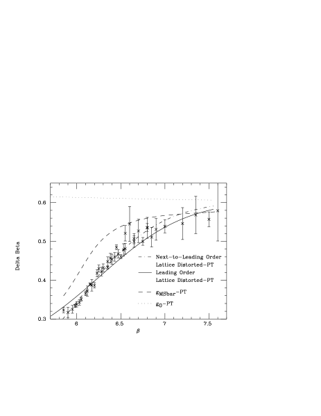
Figure 7: Plot of $\Delta\beta(\beta)$ together with fits from various methods described in the text. In all cases the 2-loop function $f_{PT}$ was used. The Monte Carlo data points are from [25].

Figure 8: Plot of $a^{-1}/a^{-1}_{PT}$ versus $a^{2}_{PT}$ for the string tension, where $a^{-1}_{PT}=\Lambda_{L}/f_{PT}(g_{0}^{2})$. The value of $\Lambda_{L}=5.85$ MeV from table 2 was used and the 2-loop form of $f_{PT}$ was used to define $a_{PT}$.

3 Fits Using Lattice-Distorted PT

In this section we fit lattice Monte Carlo data for $\sigma,r_{0}\cite[cite]{[\@@bibref{}{sommer}{}{}]},M_{\rho},f_{\pi}$ and the $1P-1S$ splitting to the form eq.(4) with the coefficients $d^{L}$ set to zero appropriately (i.e. we ignore higher order effects in $g_{0}^{2}$). The data for these quantities is displayed in table 1 together with the references in column 1.

We perform two fits to eq.(4). The first with $f_{PT}$ defined with $d^{L}_{l-1}=0$ for $l\geq 3$ (i.e. including only 2-loop terms - see eq.(2)). The second is with $f_{PT}$ defined with $d^{L}_{l-1}=0$ for $l\geq 4$ (i.e. including the newly calculated 3-loop term, $b^{L}_{2}$ [1]).

With the exception of the $1P-1S$ splitting [7] which comes from the clover action [12, 13], we consider results only from the Wilson action [11]. This is because there is not yet a great deal of data at a wide range of $\beta$ values for non-Wilson actions.

We also fit the discrete beta function $\Delta\beta$ defined implicitly by

$$a_{L}(\beta-\Delta\beta(\beta))=2a_{L}(\beta)$$ (5)

where $a_{L}$ is again defined from eq.(4) with the same constraints on the coefficients as mentioned above. We use the $\Delta\beta$ data from the QCD-Taro collaboration [25].

In these fits we begin by including only the leading ${\cal O}(a^{n})$ term appropriate for each quantity. To be specific we rewrite eq.(4) as

$$a^{-1}_{L}(g_{0}^{2})=\frac{\Lambda_{L}}{f_{PT}(g_{0}^{2})}\times\left[1-X_{n,\nu}\frac{g_{0}^{\nu}f_{PT}^{n}(g_{0}^{2})}{f_{PT}^{n}(1)}\right],$$ (6)

where there is no implicit summation over $n$ and $\nu$. Note that the ${\cal O}(a^{n})$ coefficient has been normalised so that $X_{n,\nu}$ is the fractional amount of the ${\cal O}(g_{0}^{\nu}a^{n})$ correction at a standard value of $g_{0}=1$, corresponding of course to $\beta=6/g_{0}^{2}=6$. Also note that we have approximated the polynomial coefficient, $c^{\prime}_{n}(g_{0}^{2})$, by its leading ${\cal O}(g_{0}^{2})$ term. For each physical quantity listed above this leading term corresponds to the following values of $n$ and $\nu$:

$$M_{\rho},f_{\pi},1P-1S\;\;\;:\;\;\; \nu=0,n=1$$

$$\sigma,\Delta\beta\;\;\;:\;\;\; \nu=0,n=2$$

$$r_{0}\;\;\;:\;\;\; \nu=2,n=2.$$ (7)

The values in eq.(7) arises because different quantities have different discretisation effects. For example, $\sigma$, is measured using the gluonic part of the lattice action only, and hence is correct to ${\cal O}(a^{2})$. The scale $r_{0}$ is correct to ${\cal O}(g_{0}^{2}a^{2})$ [9], hence the values $\nu=2,n=2$ for this quantity, etc.

A simple least squares fit of each column of data in table 1 to eq.(6) provides the values for $\Lambda_{L}$, the coefficient $X_{n,\nu}$, and the $\chi^{2}$ as listed in tables 2 & 3 in the rows marked Leading-Order Lattice Distorted PT. Table 2 contains fits using the 2-loop $f_{PT}$, and table 3 has fits using the 3-loop function. In the case of $\Delta\beta$, we use eq.(5) with $a_{L}$ defined in eq.(6).

Also shown in tables 2 & 3 are the fits to 2-loop and 3-loop $g_{0}$-PT. We see that leading order lattice-distorted PT fits the data very well compared to the $g_{0}$-PT case, with the $\chi^{2}/dof$ down by up to two orders of magnitude. Figures 2-7 display the above fits in the case of the 2-loop fit.

As a further check of the method, we include in the fit the next-to-leading term in $a$. However, due to the large statistical errors in some of the lattice data we perform this fit only for $\sigma,r_{0}$ and $\Delta\beta$ where the statistical errors are very small. The fitting function in these cases is:

$$a^{-1}_{L}(g_{0}^{2})=\frac{\Lambda_{L}}{f_{PT}(g_{0}^{2})}\times\left[1-X_{n,\nu}\frac{g_{0}^{\nu}f_{PT}^{n}(g_{0}^{2})}{f_{PT}^{n}(1)}-X_{n,\nu+2}\frac{g_{0}^{\nu}f_{PT}^{n+2}(g_{0}^{2})}{f_{PT}^{\;n+2}(1)}\right].$$

The results of these fits are again displayed in tables 2 & 3 for the 2-loop and 3-loop cases. The figures 3 and 7 also display the fit in the 2-loop case for $r_{0}$ and $\Delta\beta$.

Obviously in the limit of infinite statistical precision, reasonable fits to the lattice-distorted PT formula would only be obtained if the ${\cal O}(a^{n})$ terms were included to all orders. The fact that it is necessary to go to next-to-leading order for the $\sigma$, $r_{0}$ and $\Delta\beta$ data to obtain a sensible $\chi^{2}/dof$ simply states that these data have sufficiently small statistical errors to warrant this order fit. From here on, we take the results of the next-to-leading order fits to the $\sigma$, $r_{0}$ and $\Delta\beta$ data as our best fits for these quantities.

Some comments about the lattice-distorted PT procedure are necessary.

• The most important point is that for the $\sigma,r_{0}$ and $\Delta\beta$ data, the agreement between the data and lattice-distorted PT is truly remarkable considering the tiny statistical errors in the lattice data.

• Another important finding is that the values of $\Lambda_{L}$ for the various quantities in the 3-loop case are all consistent with $\Lambda_{L}=7.7$ MeV within $1\sigma$. The only exception is the string tension. Since the “experimental” value of the string tension requires certain model assumptions, it is not possible to draw any firm conclusion from this last observation. While the effects of quenching will mean that, at some level, the various values of $\Lambda_{L}$ will not all coincide, it is encouraging that the $\Lambda_{L}$ values agree to $\sim 10\%$ . We take $\Lambda_{L}=7.7\pm 10\%$ MeV as an overall average where the error includes an estimate (obtained by a comparison of the 2 and 3-loop fits) of the effect of the unknown higher order terms $b^{L}_{3}$, $b^{L}_{4}$ etc. Using $\Lambda_{\overline{MS}}=28.81\times\Lambda_{L}$, [26], we have,

  $$\Lambda^{N_{f}=0}_{\overline{MS}}=220\pm 20\;\;\;\mbox{MeV},$$

  where the superscript $N_{f}=0$ refers to the quenched approximation. This compares very well with other lattice determinations of $\Lambda^{N_{f}=0}_{\overline{MS}}$ [27] and therefore is support for the validity of this approach.

• The typical values of $X_{n,\nu}$ in table 2 is 20-40%. In [28], it was found that non-perturbative determinations of the renormalisation constant of the local vector current, $Z^{Ren}_{V}$, vary by 10-20% depending on the matrix element used. This spread in $Z^{Ren}_{V}$ has been interpreted as ${\cal O}(a)$ effects [13]. Note that the simulation in [28] was at $\beta=6.4$ where the value of $a$, and hence the size of the ${\cal O}(a)$ term, is around half that at $\beta=6.0$. Thus the values we obtain for $X_{n,\nu}$ in this study are directly comparable with the ${\cal O}(a)$ effects already uncovered in [28], confirming the lattice-distorted PT picture.

• A compelling plot supporting lattice-distorted PT is shown in figure 8. In this graph $a^{-1}_{\sigma}/a^{-1}_{PT}$ is plotted against $a^{2}_{PT}$, where $a^{-1}_{PT}=\Lambda_{L}/f_{PT}(g_{0}^{2})$. The 2-loop form of $f_{PT}$ is used, however, in this plot, the 3-loop would be indistinguishable. The value of $\Lambda_{L}=5.85$ MeV from table 2 is used. If $g_{0}$-PT were correct (i.e. if there were perturbative scaling) then the behaviour would be constant. Clear evidence for linear behaviour with non-zero slope is apparent, implying that the dominant corrections to $g_{0}$-PT are of ${\cal O}(a^{2}_{PT})$.

• The coefficients for the second order terms, $X_{n,\nu+2}$ are an order of magnitude smaller than the first order terms, $X_{n,\nu}$. This follows our expectation that the expansion in $f_{PT}$ in eq.(4) forms a convergent series, and that the bulk of the cut-off effects at present values of $\beta$ are due to the leading order term.

• One of the most exciting features of the lattice-distorted PT approach is that it can reproduce the behaviour of $\Delta\beta$ (see fig.7). 3-loop $g_{0}$-PT predicts

  $$\Delta\beta(\beta)=\delta_{0}+\delta_{1}g_{0}^{2}+\delta^{L}_{2}g_{0}^{4}$$ (8)

  with $\delta_{0}=12b_{0}\log 2$, $\delta_{1}=12b_{1}\log 2$ and $\delta^{L}_{2}=12b^{L}_{2}\log 2$. The dotted curve in figure 7 with a near constant value of around 0.6, shows the behaviour predicted from 2-loop $g_{0}$-PT. (The 3-loop term, $\delta_{2}g_{0}^{4}$ brings this curve down by only around 2%.) The large discrepancy between lattice Monte Carlo data and 2-loop $g_{0}$-PT for $\Delta\beta$ has long been noted [29]. The conventional reason for this “dip” is that it is a remnant of the line of first order phase transitions in the fundamental-adjoint coupling plane which ends near the fundamental axis in the vicinity of this dip [30]. However, the lattice-distorted PT can clearly solve this problem without resorting to other explanations.

  Note in [25], a fit was performed to their $\Delta\beta$ data using two free parameters. The first was a 3-loop coefficient $\delta_{2}$ (see eq.(8)), and the second involved defining a renormalised coupling, $g_{u}$, with a shift $c_{0}$ relative to the $g_{\overline{MS}}$ coupling [7],

  $$\frac{6}{g_{u}^{2}} = \frac{6}{g_{\overline{MS}}^{2}}-c_{0}$$

  $$= \frac{6<U_{Plaq}>}{g_{0}^{2}}+0.15-c_{0}.$$

  A good fit was obtained with a sensibly small 3-loop term, $\delta_{2}/\delta_{0}=-0.013(1)$, but with a huge shift $c_{0}=2.61(4)$ which is unphysical since it leads to a divergent value of $g_{u}^{2}$ at $\beta=6/g_{0}^{2}\approx 5$ [25]. Thus this attempt at reconciling the $\Delta\beta$ data with PT proved unsuccessful.

• Comparing the values of $X_{n,\nu}$ and $X_{n,\nu+2}$ in the 2 and 3-loop cases (i.e. tables 2 & 3) we see that they are compatible. In fact the main changes between the 2 and 3-loop cases are in the values of $\Lambda_{L}$ which increases by around 15-20%. This variation is consistent with the value of $d^{L}_{2}$ (see eq.(2)). In other words, the term $d^{L}_{2}g^{2}$ can be well approximated by $d^{L}_{2}$. This again implies that the higher order terms in $g_{0}^{2}$ are not important in the comparison between perturbation theory and current Monte Carlo data (apart from a normalising effect on $\Lambda_{L}$).

• The values of $X_{n,\nu}$ and $X_{n,\nu+2}$ in the case of $\sigma$ are compatible with those for $\Delta\beta$. This is a comforting feature, since both quantities are, in effect, obtained from the study of large Wilson loops [25].

• As far as the fit to $M_{\rho},f_{\pi}$ and the $1P-1S$ splitting are concerned, the errors in the lattice data are large enough to allow many functional forms. Thus these data do not constrain the lattice-distorted PT fit (or fits from other schemes).

• The coefficients $c^{\prime}_{n}$ of the ${\cal O}(a^{n})$ terms in eq.(4) are, strictly speaking, polynomial functions of $g_{0}^{2}$. In the above fits, we have taken only the leading term in this polynomial. This is consistent with the lattice-distorted PT approach, since it assumes that the leading term of ${\cal O}(a^{n})$ appearing in eq.(4) dominate the ${\cal O}(g_{0}^{2l-4})$ terms. Consistency within this picture therefore implies that the polynomials $c^{\prime}_{n}(g_{0}^{2})$ can be replaced with their leading term in $g_{0}^{2}$.

• The errors in the fitting parameters $X_{n,\nu}$ are statistical only. They do not include any estimate of the systematic error due to the non-inclusion of the still higher order terms in $a$. A more refined fitting procedure would be required to estimate these errors. This will be left for future studies.

• The renormalisation constant used in the determination of $a^{-1}_{f_{\pi}}$ is $Z^{Ren}(g_{0}^{2})=1-0.132g_{0}^{2}$ [31] i.e. for consistency we have used the bare lattice coupling as the expansion parameter, rather than a renormalised coupling. However, as already mentioned, the statistical errors in the data for $a^{-1}_{f_{\pi}}$ are too large to enable useful conclusions to be drawn from these data alone.

4 Fits Using a Renormalised Perturbation Theory

4.1 Introduction to the Renormalised Coupling fits

In this section we fit the Monte Carlo data for $a^{-1}$ to the following functional form:

$$a^{-1}_{L}(g_{0}^{2})=\frac{\Lambda}{f_{PT}((g^{\prime})^{2})},$$ (9)

where $g^{\prime}$ is some “renormalised” coupling which is in turn a function of the bare coupling $g_{0}$.

Note that the philosophy behind these fits is that the failure of asymptotic (perturbative) scaling is explained by higher order terms in perturbation theory. The coupling $g^{\prime}$ is defined with the aim of creating perturbative series with improved convergence properties. This is an orthogonal philosophy compared to the procedure outlined in Sect. 3 where finite lattice spacing errors are assumed to cause the disagreement between Monte Carlo data and perturbative scaling. (Note that the ${\cal O}(a^{n})$ terms in eqs.(6 & 3) cannot be expressed as polynomials in $g_{0}^{2}$ - i.e. they cannot be written in the form of the $d^{L}_{l-1}g_{0}^{2l-4}$ terms in eq.(4).)

The following subsections study fits using various definitions of $g^{\prime}$. Both 2 and 3-loop fits were performed, analogous to the lattice distorted case. At the end of this section we make some general comments about the success or otherwise of the renormalised coupling approach.

4.2 Fits Using $g_{\overline{MS}}$-Perturbation Theory

Following ref. [7] we define an ${\overline{MS}}-$like coupling, where $g^{\prime}=g_{\overline{MS}}$,

$$\frac{1}{g_{\overline{MS}}^{2}(\pi/a)}=\frac{1}{g_{0}^{2}}\;<\frac{1}{3}TrU_{plaq}>_{MC}+0.025.$$

The results of using this definition of $g^{\prime}$ in the fitting function Eq.(9) (with the 2-loop definition of $f_{PT}$) are displayed in Figs 2 - 7 and in Table 2 in the rows headed $g_{\overline{MS}}$.

In order to perform 3-loop fits, an extra fitting parameter, $d^{\overline{MS}}_{2}$, in $f_{PT}$ is required. This is because $d^{L}_{2}$ from [1] is only appropriate for the $g_{0}$ scheme. The results of these fits are displayed in Table 4.

4.3 Fits Using $g_{V}$-Perturbation Theory

We now turn to some definitions of $g^{\prime}$ proposed by Lepage and Mackenzie [4]. Ref. [4] lists three alternative “renormalised” couplings $g_{V}^{(i)}$ ($i=I,II,III$) which are based on, or related to the strength of the static quark anti-quark potential. They are:

$$\alpha_{V}^{(I)}(\pi/a)=\frac{\alpha_{L}}{<\frac{1}{3}TrU_{plaq}>_{MC}}\times(1+0.513\alpha_{V}),$$

(see [4] eq(29)); and

$$-\ln{<\frac{1}{3}TrU_{plaq}>_{MC}}=\frac{4\pi}{3}\alpha_{V}^{(II)}(3.41/a)\times(1-1.19\alpha_{V}),$$

(see [4] eq(20)); and

$$\alpha_{V}^{(III)}(46.08/a)=\alpha_{L},$$

(see [4] eq(30)) where $\alpha\equiv g^{2}/4\pi$ throughout and $MC$ stands for Monte Carlo estimate. Lepage and Mackenzie argue that all three definitions agree up to ${\cal O}(\alpha_{V}^{3})$ (see discussion surrounding Fig. 7 of Ref. [4]).

Before checking the fits of $a^{-1}$ using these definitions of $g_{V}$, we briefly discuss the effects of the momentum scale in the above definitions. Lepage and Mackenzie argue that there is a momentum scale $q^{\ast}$ which is most appropriate for each quantity studied which can be obtained from a mean field calculation. Thus, for example, the $q^{\ast}$ value for the critical quark mass for the Wilson action is $q^{\ast}=2.58/a$. In order to fit the Monte Carlo data for $a^{-1}$ to Eq. (9) (with $g^{\prime}=g_{V}$), we should, in theory, first obtain a value for $q^{\ast}$ appropriate for each of the quantities $\Omega$ studied ($\Omega=\sigma,r_{0},M_{\rho},f_{\pi},$ or the $1P-1S$ splitting). However, as is shown below, fits using Eq. (9) are not dependent on the scale $q^{\ast}$ chosen, so long as the parameter $\Lambda_{V}$ is trivially rescaled.

We prove this statement as follows. Since $g_{V}$ is a function of $q$ and $\beta$, we write $g_{V}(q,\beta)$ to make these dependencies explicit. In order to calculate the coupling, $g_{V}(q^{\ast},\beta)$, at some new scale, $q^{\ast}$, we first must determine $\Lambda_{V}$. This can be done using

$$\Lambda_{V}=q\;f_{PT}(g_{V}^{2}(q,\beta)).$$ (10)

Once $\Lambda_{V}$ has been determined, the value of $g_{V}$ can be determined at the new scale $q^{\ast}$ using the implicit definition:

$$\Lambda_{V}=q^{\ast}\;f_{PT}(g_{V}^{2}(q^{\ast},\beta)).$$ (11)

Now we turn to the fit of the $a^{-1}_{L}$ obtained from a Monte Carlo determination of some physical quantity $\Omega$. The appropriate fitting function (see Eq.(9)) is

$$a^{-1}_{L}(g_{0}^{2})=\frac{\Lambda_{V}}{f_{PT}(g^{2}_{V}(q^{\ast},\beta))}\;.$$

Using Eqs.(10 & 11) we immediately have

$$a^{-1}_{L}(g_{0}^{2})=\frac{q^{\ast}/q\;\Lambda_{V}}{f_{PT}(g^{2}_{V}(q,\beta))}=\frac{\Lambda^{\prime}_{V}(q)}{f_{PT}(g^{2}_{V}(q,\beta))}\;,$$ (12)

where $\Lambda^{\prime}_{V}(q)\equiv\frac{q^{\ast}}{q}\Lambda_{V}$. So the fit is independent of the choice of $q^{\ast}$ apart from a trivial rescaling of $\Lambda_{V}$, as claimed. Therefore we do not need to worry about the choice of $q^{\ast}$ for the quantities $\Omega$ considered in this study. Note, however, that for quantities such as the plaquette which perturbatively are expressed as a polynomials in $g^{2}$ rather than proportional to $f_{PT}$, the above argument does not hold, and results do depend on the choice of $q^{\ast}$. This last fact has been shown in Ref. [4].

The results of the fits of the $a^{-1}$ data to the functional form in Eq. (12) (with the 2-loop definition of $f_{PT}$) are shown in Table 2 in the rows headed $g_{V}^{(I,II)}$. The coupling $g_{V}^{(III)}$ was not considered since it would be the lead to the same fit as the $g_{0}$ case apart from a trivial constant factor in the $\Lambda_{V}$ value as discussed above. The $q$ values for the fits $I,II$ are $q=\pi/a,\,3.41/a$ respectively. Since it is only the quality of the fits that is of interest no attempt was made to run the coupling $g_{V}^{(I,II)}$ to the same momentum scale. However if this was attempted, inconsistent results would be obtained, since the $\Lambda^{\prime}_{V}(q)$ values do not appear to fit the relationship $\Lambda^{\prime}_{V}(q^{(I)})\equiv\frac{q^{(II)}}{q^{(I)}}\Lambda^{\prime}_{V}(q^{(II)})$.

As in the ${\overline{MS}}$ case, in order to perform 3-loop fits, an extra fitting parameter, $d^{V}_{2}$, in $f_{PT}$ is required. The results of these fits are displayed in Table 4.

4.4 Fits Using $g_{E}$-Perturbation Theory

Following refs. [3] and [5] we define a coupling, $g_{E}$, based on the plaquette,

$$\frac{1}{g_{E}^{2}}=\frac{c_{1}}{1-<\frac{1}{3}TrU_{plaq}>_{MC}}.$$

where $c_{1}=\frac{1}{3}$ is the coefficient of the first term in the perturbative expansion for $1-<\frac{1}{3}TrU_{plaq}>$. The results using this definition for $g^{\prime}$ in the fitting function eq.(9) are displayed in Table 2 in the rows headed $g_{E}$-PT for the case of the 2-loop fits. For the 3-loop fit, the coefficient appropriate for the $g_{E}$ scheme can be derived from a short calculation [1], $d^{E}_{2}=0.01161$. The results for these fits are displayed in Table 3.

In ref [5], the $g_{E}$ scheme was extended to the next order in the perturbation series. That is, a coupling $g_{E2}$, is defined by demanding that the Monte Carlo result for the plaquette is equal to the perturbative series truncated to second order. i.e.

$$1-<\frac{1}{3}TrU_{plaq}>_{MC}=c_{1}g_{E2}^{2}+c_{2}g_{E2}^{4},$$

where $c_{2}=2\times(0.0204277-1/288)$ [32]. The results of this fit are displayed in Table 2 in the rows headed $g_{E2}$ for the 2-loop fit. As in the ${\overline{MS}}$ case, in order to perform 3-loop fits, an extra fitting parameter, $d^{E2}_{2}$, in $f_{PT}$ is required. The results of these fits are displayed in Table 4.

4.5 Discussion of the Renormalised Coupling fits

We begin with a discussion on the quality of the fits in the 2-loop case. As can be seen from Table 2, the fits using $g_{\overline{MS}}$, $g_{V}^{I}$, $g_{V}^{II}$, $g_{E}$ and $g_{E2}$ -PT are not as successful as those from lattice distorted-PT. It is interesting to note that of the two $g_{V}$ fits, the $g_{V}^{II}$ definition seems more successful. Surprisingly, the $g_{E2}$ fit is not a great deal better than the $g_{E}$ fit, even though it should naively be correct to one more order of perturbation theory. This in itself suggests that pushing to higher orders in perturbation theory does not pay significant dividends.

Concentrating on the fits to $\sigma$, $r_{0}$ and $\Delta\beta$ where the lattice data has very small statistical errors, we see from Table 2 that the $g_{V}^{II}$ and the $g_{E2}$ -PT methods are the most successful of the renormalised coupling approaches. In fact the $g_{V}^{II}$ and $g_{E2}$ -PT fits to $r_{0}$ are comparable in quality to the leading-order lattice distorted PT. However, these same $g_{V}^{II}$ and $g_{E2}$ fits are an order of magnitude worse for the $\sigma$ case compared to the leading-order lattice distorted PT, and are also significantly worse for the fits to $\Delta\beta$.

Of course the (leading order) lattice distorted PT fits include one extra fitting parameter ($X_{n,\nu}$) compared to the renormalised coupling fits, so it is tempting to argue that the former fits are more successful only for this reason. However, Sec.3 details the results from a renormalised coupling style fit with two extra fitting parameters that proved entirely unsuccessful [25].

Turning to the 3-loop case, even more striking comments can be made. While it remains true that the lattice distorted PT fits remain stable and of high quality, the same cannot be said for the renormalised coupling approach. The $g_{E}$ scheme (whose 3-loop coefficient is known) cannot reproduce the quality of fits of the (even) the leading order lattice distorted PT (see Table 3). Furthermore, of the four schemes listed in Table 4, none can provide sensible fits for all the quantities studied. A “sensible fit” is defined, very liberally, as one where the fitted value for $d_{2}$ lies in the range $0\leq d_{2}\leq 1$. Note also that in the cases where sensible fits are obtained, the values of $d_{2}$ depend strongly on the quantity being studied - a clear indication that there are non-universal (finite-lattice spacing) effects present. Furthermore, the values of the coefficient $d_{2}$ can often be $\sim 20\%$ or more. According to the renormalised coupling philosophy, $d_{2}$ should be significantly smaller than the corresponding coefficient in the $g_{0}$ scheme. However, since $d^{L}_{2}\sim 20\%$, this is clearly not the case.

In conclusion none of the renormalised coupling methods approach the quality and consistency of the fits from lattice distorted PT method.

5 Discussion & Conclusions

In this paper we discuss the possible causes of the lack of perturbative scaling in dimensionful lattice quantities. We have argued that the cause of this disagreement is due to either (i) the neglect of higher order terms in perturbation theory (i.e. the renormalised coupling approach), and/or (ii) the presence of cut-off effects due to the finiteness of the lattice spacing, $a$ (i.e. the lattice distorted PT approach). Taking a collection of quenched lattice data from various collaborations for the string tension $\sigma$, the hadronic scale $r_{0}$, $M_{\rho}$, $f_{\pi}$, the $1P-1S$ splitting in charmonium and the discrete beta function $\Delta\beta$, we have attempted fits assuming each of the hypotheses (i) and (ii) above. We have found that modelling the discrepancy using (i), through the use of a renormalised coupling, $g^{\prime}$, provides less satisfactory fits to the data compared to (ii). In fact, the hypothesis (ii) leads to a remarkable consistency both in the fitted $\Lambda$ parameters and amongst the sizes of the ${\cal O}(a^{n})$ corrections. Furthermore, the hypothesis (ii) succinctly explains the “non-perturbative” behaviour of $\Delta\beta$. This, we feel, is one of its major achievements. Using the fits from lattice distorted PT (method (ii)) we estimate $\Lambda^{N_{f}=0}_{\overline{MS}}=220\pm 20$ MeV, perfectly compatible with values obtained from other methods. We find excellent consistency for this $\Lambda_{\overline{MS}}$ value amongst the different physical quantities studied.

It is clear however, that we have not proven that the lack of perturbative scaling is due to finite lattice spacing effects (i.e. hypothesis (ii)). In fact, presumably, the true state of affairs is that the lack of perturbative scaling is due to a mixture of the two effects (i) and (ii). However, we have given strong arguments to support the claim that the discrepancy between the perturbative scaling formula and current Monte Carlo data is dominated by lattice artifacts (see Sec.3).

Figure 9: Plot of $a^{-1}/a^{-1}_{PT}$ versus $a_{PT}$ and $g_{0}^{2}$. The string tension is used to set $a$. $a_{PT}$ is defined as $\Lambda_{L}/f_{PT}(g_{0}^{2})$ where $\Lambda_{L}=5.85$ MeV is taken from Table 2 and the 2-loop version of $f_{PT}$ is used. The data points are plotted using diamonds (the error bars are suppressed since they are smaller than the symbols). The vertical lines joining them to the $a_{PT}-g_{0}^{2}$ axis are guides for the eye only. The curves in the $a_{PT}-g_{0}^{2}$ plane are $a_{PT}=f_{PT}(g_{0}^{2})/\Lambda_{L}$ with $\Lambda_{L}$ defined as above. (No discernible difference in this plot would be observed if the 3-loop version of $f_{PT}$ were used instead.)

A pictorial representation of the approach to perturbative scaling in lattice data is displayed in Figure 9. Here the ratio $a^{-1}_{\sigma}/a^{-1}_{PT}$ is plotted on a 3-dimensional graph against both $g_{0}^{2}$ and $a_{PT}$. $a^{-1}_{\sigma}$ is defined from the Monte Carlo values for the string tension (from Table 1), and $a_{PT}$ is defined, $a^{-1}_{PT}(g_{0}^{2})=\Lambda_{L}/f_{PT}(g_{0}^{2})$, where $\Lambda_{L}=5.85$ MeV is taken from Table 2. (In the actual plot the 2-loop formula for $f_{PT}$ has been used. However, the 3-loop plot would be indistinguishable.) We use the string tension in this graph since the lattice data has very small statistical errors, however other quantities would lead to similar plots. The diamonds are the data points (error bars have been omitted because they are smaller than the symbols), and the vertical lines joining the data points to the $a_{PT}-g_{0}^{2}$ plane are guides for the eye only. The two curves shown are defined by $a_{PT}(g_{0}^{2})=f_{PT}(g_{0}^{2})/\Lambda_{L}$, with $\Lambda_{L}$ defined as above. The lower curve is a guide for the eye, and the upper curve is in the $a^{-1}_{\sigma}/a^{-1}_{PT}=1$ plane. This upper curve shows the relationship between the Monte Carlo derived lattice spacing, $a$, the bare coupling, $g_{0}^{2}$, and the perturbative formula for the lattice spacing, $a_{PT}$ in the idealised case of perfect (2-loop) perturbative scaling. It is important to note that the deviation between the data points and this curve in Figure 9 is precisely the discrepancy being studied in this paper.

The ratio $a^{-1}_{\sigma}/a^{-1}_{PT}$ is interesting since from eq.(4) it is unity up to terms ${\cal O}(g_{0}^{2})$ and ${\cal O}(a_{PT})$, i.e.

$$\frac{a^{-1}_{\sigma}}{a^{-1}_{PT}}=(1+\sum_{l=4}d^{L}_{l-1}g_{0}^{2l-4})^{-1}\times(1+\sum_{n=1}c^{\prime}_{n}(g_{0}^{2})a_{PT}^{n}(g_{0}^{2})).$$ (13)

From Figure 9 the ratio $a^{-1}_{\sigma}/a^{-1}_{PT}$ varies from 0.6 to around 1.0 over the range of presently available lattice data. It can also be seen that the range in $a_{PT}$ available from current lattice data spans a factor of 3-4, whereas the corresponding range in $g_{0}^{2}$ is very small - from around 0.88 to 1.05 only (i.e. a spread of $\;\raisebox{-2.15277pt}{\hbox to0.0pt{$\sim$\hss}}\raisebox{2.15277pt}{$<$}\;20\%$). Thus, the best of the current data is relatively a long way from the continuum limit $a=g_{0}^{2}=0$ in terms of variable $g_{0}^{2}$, but apparently relatively close in terms of $a$. Therefore current lattice data is in the regime where effects of ${\cal O}(a)$, ${\cal O}(a^{2})$ etc, will be seen clearly (if these terms are significant) since there is a broad range in $a$ available. Conversely, higher order effects in $g_{0}^{2}$ will be much more difficult to discern since the range available in this variable is so compact.

We now aim to reconcile the rapid variation of $a^{-1}_{\sigma}/a^{-1}_{PT}$ from 0.6 to around 1.0 with eq.(13). Considering the relative variations in $g_{0}^{2}$ and $a_{PT}$, it is natural to assume that the ${\cal O}(a^{n})$ term (with $n=2$ for the string tension) is more dominant than the ${\cal O}(g_{0}^{2})$ term. Note that the fact that significant ${\cal O}(a)$ corrections have already been uncovered in lattice data adds support to these arguments (see Sec.3).

To be more quantitative, we have performed a fit of the form

$$\frac{a^{-1}_{\sigma}}{\Lambda_{L}/f_{PT}(g_{0}^{2})}=(1+d^{L}_{3}g_{0}^{4})^{-1}\times(1+c^{\prime}_{2}a_{PT}^{2}(g_{0}^{2})),$$

to the $\sigma$ and $r_{0}$ data in table 1. Obviously this fitting form allows both an ${\cal O}(a^{2})$ distortion, and a 4-loop correction. The result is a worse fit than the next-to-leading order lattice distorted fit (which has the same number of free fitting parameters) in the case of the $\sigma$ data, and no sensible fit at all in the case of the $r_{0}$ data.

Of course this argument again does not prove the case for lattice distorted PT; one could rely on the conspiracy of higher order terms in perturbation theory to recover the behaviour seen in Figure 9 without the need for any ${\cal O}(a^{n})$ terms at all. However, it seems much more natural, taking into account the arguments outlined above and in Sec.3, to rely on the ${\cal O}(a^{n})$ terms to explain the discrepancy instead.

Using these assumptions, we can determine the value of the coupling when the finite lattice spacing effects first drop below, say, 1%. Taking a typical value of $X_{n,\nu}\approx 30\%$ from Table 2 or 3, the ${\cal O}(a^{n})$ term in eq.(6), $\approx X_{n}f_{PT}^{n}(g_{0}^{2})/f_{PT}^{n}(1)$, is less than 1% for $g_{0}^{2}\;\raisebox{-2.15277pt}{\hbox to0.0pt{$\sim$\hss}}\raisebox{2.15277pt}{$<$}\;0.7$, i.e. $\beta\;\raisebox{-2.15277pt}{\hbox to0.0pt{$\sim$\hss}}\raisebox{2.15277pt}{$>$}\;9$ in the case of $n=1$ distorted quantities, and for $g_{0}^{2}\;\raisebox{-2.15277pt}{\hbox to0.0pt{$\sim$\hss}}\raisebox{2.15277pt}{$<$}\;0.8$, i.e. $\beta\;\raisebox{-2.15277pt}{\hbox to0.0pt{$\sim$\hss}}\raisebox{2.15277pt}{$>$}\;8$ for $n=2$ quantities.

Continuing the assumption that the discrepancy between lattice data and perturbative scaling is due to finite lattice spacing effects, we can also explain why it is that the renormalised coupling approach works as well as it does. This is presumably because the ${\cal O}(a)$ effects of the quantity being used to define $g^{\prime}$ are embedded in the definition of $g^{\prime}$. So long as the ${\cal O}(a)$ effects in the quantity being used to define $g^{\prime}$ are similar in sign and magnitude to those in the quantity being studied (e.g. $\sigma$, $r_{0}$, etc.) the PT expressed in terms of $g^{\prime}$ will fit the lattice data better than the bare $g_{0}$ formula. Thus the $g^{\prime}$ definition mixes finite lattice spacing distortions with higher order perturbative effects.

There is a final interesting opportunity assuming the correctness of the lattice distorted perturbative scaling philosophy [6]. Suppose one is studying the continuum limit of a dimensionful quantity, $\Omega$, using lattice estimates determined at a set of finite $a$ values. Typical examples of $\Omega$ are the pseudoscalar decay constant $f_{\pi}$ or the mass $M_{\rho}$. The physical value of $\Omega$ can be written as

$$\Omega=\lim_{g_{0}\rightarrow 0}\;[Z^{Ren}(g_{0}^{2})\times\Omega^{\#}(g_{0}^{2})\times a^{-1}(g_{0}^{2})]$$ (14)

where $Z^{Ren}$ is the renormalisation constant appropriate for $\Omega$ (which is unity in the case of hadronic masses), and $\Omega^{\#}$ is the (dimensionless) lattice value for $\Omega$. The limit $g_{0}\rightarrow 0$ simply expresses the fact that the physical value is obtained by taking the continuum limit of the lattice estimates. Assuming that there is no phase transition between values of $g_{0}^{2}$ used in present lattice calculations and $g_{0}=0$, we can write eq.(14) as

$$\Omega=[\lim_{g_{0}\rightarrow 0}Z^{Ren}(g_{0}^{2})]\times\lim_{g_{0}\rightarrow 0}[\Omega^{\#}(g_{0}^{2})\times a^{-1}(g_{0}^{2})]$$

For quantities where $Z^{Ren}(g_{0}^{2})$ can be expressed as polynomial in $g_{0}^{2}$ (such as decay constants and hadronic masses) we have

$$\Omega=Z^{Ren}(g_{0}^{2}=0)\times\frac{\Lambda_{L}}{\lambda_{\Omega}}$$ (15)

where we have fitted $a^{-1}$ according to eq.(6) or eq.(3), and we have fitted $\Omega^{\#}$ along similar lines as follows,

$$\frac{1}{\Omega^{\#}(g_{0}^{2})}=\frac{\lambda_{\Omega}}{f_{PT}(g_{0}^{2})}\times\left[1-X_{n,\nu}\frac{g_{0}^{\nu}f_{PT}^{n}(g_{0}^{2})}{f_{PT}^{n}(1)}\right].$$

Typically $Z^{Ren}(g_{0}^{2}=0)$ is known immediately, without the need for any calculation, (e.g. it is unity for decay constants and hadronic masses). This means that the continuum estimate of $\Omega$ can be found using eq.(15) simply via two lattice distorted PT style fits.

References

- [1] B. Allés, A. Feo and H. Panagopoulos, hep-lat/9609025.
- [2] S. Caracciolo, R.G. Edwards, A. Pelissetto and A.D. Sokal, Phys. Rev. Lett. 75 (1995) 1891.
- [3] G. Parisi, in High Energy Physics -1980, Proceedings of the XXth International Conference, Madison, Wisconsin, 1980, edited by L. Durand and L.G. Pondrom, AIP Conf. Proc. No. 68 (AIP, New York, 1981), p. 1531.
- [4] G.P. Lepage and P.B. MacKenzie, Phys.Rev. D48 (1993) 2250.
- [5] G.S. Bali and K. Schilling, Phys.Rev. D47 (1993) 661
- [6] C.R. Allton, Nucl.Phys. B437 (1995) 641.
- [7] A.X. El-Khadra, G.M. Hockney, A.S. Kronfeld and P.B. Mackenzie, Phys.Rev.Lett. 69 (1992) 729.
- [8] C. W. Bernard, Nucl. Phys. B (Proc. Suppl.) 34 (1994) 47
- [9] R. Sommer, Nucl. Phys. B411 (1994) 839
- [10] C. Allton, talk presented at Lat96, St. Louis, SWAT/128, to appear in Nucl. Phys. B (Proc. Suppl.)
- [11] K.G. Wilson, in New Phenomena in Sub-Nuclear Physics, ed. A. Zichichi (Plenum, New York, 1977)
- [12] B. Sheikholeslami and R. Wohlert, Nucl.Phys. B259 (1985) 572.
- [13] G. Heatlie, C.T. Sachrajda, G. Martinelli and C. Pittori, Nucl.Phys. B352 (1991) 266.
- [14] A.X. El-Khadra, Nucl. Phys. B (Proc. Suppl.) 26 (1992) 372.
- [15] G.S. Bali, WUB-93-37, hep-lat/9311009, Presented at Workshop on High Energy Physics, Protvino, Russia, Sep 14-17, 1993.
- [16] K.D. Born et al, Nucl. Phys. B (Proc. Suppl.) 20 (1991) 394, as analysed by R. Sommer in [18]
- [17] F. Butler, H. Chen, J. Sexton, A. Vaccarino and D. Weingarten, Nucl. Phys. B430 (1994) 179 and Nucl. Phys. B421 (1994) 217
- [18] C. Alexandrou et al, Nucl. Phys. B414 (1994) 815
- [19] UKQCD Collab, talk presented by H. Wittig, Nucl. Phys. B (Proc. Suppl.) 42 (1995) 288, as updated by H. Wittig priv. comm.
- [20] APE Collaboration, C.R. Allton et al., Nucl.Phys. B413 (1994) 461.
- [21] APE Collaboration, talk presented by F. Rapuano, Nucl.Phys. (Proc. Suppl.) B34 (1994) 360.
- [22] APE Collaboration, talk presented by C.R. Allton, Nucl.Phys. (Proc. Suppl.) B42 (1995) 385.
- [23] A. Abada et al, Nucl. Phys. B376 (1992) 172
- [24] UKQCD Collab (S.P.Booth et al), Phys. Lett. B294 (1992) 385.
- [25] QCD-TARO Collaboration, K. Akemi et al, Nucl. Phys. B(Proc.Suppl.) 34 (1994) 246
- [26] R. Dashen and D.J. Gross, Phys. Rev. D23 (1981) 2340.
- [27] see eg., C.T.H. Davies et al., Phys. Lett. B345 (1995) 42 and [7]
- [28] A. Abada et al, Nucl.Phys. B416 (1994) 675.
- [29] see P. Hasenfratz, ‘Monte Carlo Renormalization Group Methods and Results in QCD’ CERN-TH-3999/84, Aug 1984. 47pp. Lectures given at Int. School of Subnuclear Physics, Erice, Italy, Aug 5-15, 1984. Published in Erice Subnuclear 1984:225, and references therein.
- [30] see eg., K.C. Bowler et al., Nucl. Phys. B257 (1985) 155; A. Patel et al., Phys. Rev. Lett. 57 (1986) 1288; A. Patel, R. Gupta, Phys. Lett. B183 (1987) 193; U.M. Heller, Phys. Lett. B362 (1995) 123.
- [31] G. Martinelli and Y.C. Zhang, Phys. Lett. B123 (1983) 433, R. Groot, J. Hoek and J. Smit, Nucl. Phys. B237 (1984) 111.
- [32] A. DiGiacomo and G.C. Rossi, Phys. Lett. B100 (1981) 481; A. DiGiacomo and G. Paffuti, Phys. Lett. B108 (1982) 327; U. Heller and F. Karsch, Nucl. Phys. B251 (1985) 254.