Preprint PUPT-1649

e-Print Archive: hep-lat/9610013

Curing $O(a)$ Errors in 3-D Lattice SU(2)$\times$U(1) Higgs Theory

Guy D. Moore

Princeton University

Joseph Henry Laboratories, PO Box 708

Princeton, NJ 08544, USA

Abstract

We show how to make $O(a)$ corrections in the bare parameters of 3-D lattice SU(2)$\times$U(1) Higgs theory which remove $O(a)$ errors in the match between the infrared behavior and the infrared behavior of the continuum theory. The corrections substantially improve the convergence of lattice data to a small $a$ limit.

PACS numbers: 11.15.Ha, 11.15.Kc

Keywords: Dimensional reduction, Finite spacing effects, Electroweak phase transition, Baryogenesis

1 Introduction

It is believed that the baryon number of the universe may have originated at the electroweak phase transition. The details of the mechanism depend substantially on the details of the phase transition itself, so for several years there has been growing interest in a quantitative understanding of the electroweak phase transition. Ordinary perturbation theory [1] has proven useful only when the Higgs mass $m_{H}\ll m_{W}$ the $W$ mass, and outside of this regime the only reliable methods are nonperturbative, such as lattice Monte-Carlo techniques.

The reason for the failure of perturbation theory was elucidated by the work of Farakos et. al. [2, 3, 4], who have shown how, to very good approximation, the thermodynamics of the standard model near the electroweak phase transition can be described using a three dimensional path integral for purely bosonic SU(2)$\times$U(1) Higgs theory. The theory is super-renormalizable, and hence its ultraviolet is well behaved, but its infrared is potentially nonperturbative, leading to the breakdown of perturbation theory as a tool for exploring the basically infrared physics of the phase transition. However, this same feature makes the numerical investigation of the nonperturbative physics particularly feasible; fine lattices are possible because the system is low dimensional, the couplings fall quickly with lattice spacing, and there is no need for the (numerically expensive) inclusion of fermionic degrees of freedom.

Several groups have conducted numerical experiments on the three dimensional system to study the phase transition [5, 6, 7, 8, 9, 10]. Each study used the Wilson action and the bare relations between lattice couplings and wave functions and the 3-D continuum parameters. In each case there were substantial linear in $a$ (lattice spacing) errors which had to be removed by extrapolation over several values of $a$. The extrapolation process is numerically expensive because it demands very fine lattices, and the errors in the final result are dominated by $O(a^{2})$ errors from the coarsest lattice used, and statistical errors in the finest lattices. It would be better to have an analytic understanding of the origin of the linear in $a$ corrections, which would make it possible to prevent them. One could then take data only on lattices of intermediate coarseness, obtaining smaller $O(a^{2})$ errors and better statistics with less numerical effort. This paper presents an analysis of these $O(a)$ errors.

The $O(a)$ errors in measured infrared phenomena arise because the infrared theory is clothed by interactions with more ultraviolet modes, but the clothing differs between lattice and continuum theories, both because the most ultraviolet degrees of freedom are absent on the lattice, and because the ultraviolet lattice modes have incorrect dispersion relations and extra (lattice artefact) interactions. Since the dispersion relations and couplings of the lattice theory agree with those of the continuum theory in the infrared, the difference between clothing in the two theories is all ultraviolet, and therefore perturbatively computable. Also, since the origin of the difference is ultraviolet, it should be expressible as an operator expansion, and at the desired level of accuracy only the superrenormalizable terms are needed; these can be compensated for by a shift in the bare parameters of the theory.

Dimension two operators, such as the mass squared and the $\Phi^{2}$ operator insertion, receive linearly divergent corrections at one loop; logarithmic corrections, computed in [3, 11], at two loops; and $O(a)$ corrections at three loops. The problem of determining these $O(a)$ corrections is difficult. However, if one is only interested in properties of the phase transition such as jumps in order parameters, the latent heat, the surface tension, etc. then it is not necessary to know these to high accuracy. To compute the jump in $\Phi^{2}$, for instance, one only needs to account for the multiplicative correction to the operator insertion, not the additive correction, which is common to the two phases. Similarly, precise knowledge of $m_{H}^{2}$ is only necessary to compute very precisely the equilibrium temperature. We will not pursue improvement in the determination of these quantities here, but will concentrate on improving the precision of the measurement of quantities related to the strength of the phase transition, which is more physically interesting.

The outline of the paper is as follows. In Section 2 we present the problem, establish notation, and give the results. Readers uninterested in the details of the calculation can then skip Section 3, which enumerates the required Feynman diagrams, presents the calculation of a few, and gives results for the others. The conclusion, Section 4, contains an example of using the improvement technique to reinterpret existing data. The first two appendicies contain integrals, identities, and Feynman rules needed in Section 3, and the last presents the results for the abelian Higgs model, and for the standard model but including the adjoint scalar ($A_{0}$) fields.

2 Set-up and Results

The dimensional reduction program shows that the infrared thermodynamics of the standard model are described up to small error by the partition function

$$Z = \int{\cal D}\Phi{\cal D}A_{i}{\cal D}B_{i}\exp(-\beta\int d^{3}xH)\,,$$ (1)

$$H = \frac{1}{4g^{2}}\left(F_{ij}^{a}F_{ij}^{a}+\frac{1}{\tan^{2}\Theta_{W}}f_{ij}f_{ij}\right)+(D_{i}\Phi)^{\dagger}(D_{i}\Phi)+m_{H}^{2}(\mu)\Phi^{\dagger}\Phi+\lambda(\Phi^{\dagger}\Phi)^{2}\,.$$ (2)

Here $A_{i}$ and $B_{i}$ are the gauge fields and $F^{a}_{ij}$ and $f_{ij}$ are the field strengths of the SU(2) and U(1) gauge groups respectively, and the couplings and wave function normalizations are determined with respect to physical measurables as discussed in [4]. Only $m_{H}^{2}$ depends on the ($\overline{\rm{MS}}$) renormalization point $\mu$.

The corresponding (Wilson) lattice action, in lattice units, is

$$Z = \int{\cal D}U{\cal D}u{\cal D}\Phi\exp(-\beta_{L}\sum_{x}H_{L})\,,$$ (3)

$$H_{L} = Z_{A}\sum_{i<j}(1-\frac{1}{2}{\rm Tr}P_{ij})+\frac{Z_{B}}{\tan^{2}\Theta_{W}}\sum_{i<j}(1-{\rm Re}\>p_{ij})$$ (4)

$$+Z_{\Phi}\left(\sum_{i}\left(\Phi_{a}^{2}(x)-\Phi_{a}(x)U_{iab}(x)u_{ibc}(x)\Phi_{c}(x+i)\right)+\frac{m_{HL}^{2}}{2}\Phi_{a}^{2}\right)$$

$$+\frac{(\lambda_{L}-\delta\lambda_{L})Z_{\Phi}^{2}}{4}(\Phi^{2}_{a})^{2}\,,$$

where $\Phi$ is treated as four independent real entries $\Phi_{a}$, $U$ and $u$ are the SU(2) and U(1) link variables respectively, and $P_{ij}$ and $p_{ij}$ are the SU(2) and U(1) $1\times 1$ plaquettes. The notation for $\Phi_{a}$ is equivalent to the common notation in which the Higgs field is written as a magnitude times an $SU(2)$ matrix, and each sum on $a$ is replaced by $(1/2){\rm Tr}$.

The (naive) tree relations between the lattice parameters and the 3-D continuum ones are

$$\beta_{L} \equiv \frac{4\beta}{g^{2}a}\,,$$ (5)

$$Z_{A} = 1$$ (6)

$$Z_{B} = 1$$ (7)

$$Z_{\Phi} = 1$$ (8)

$$\lambda_{L} \equiv \frac{4\lambda}{g^{2}}\,,\quad\delta\lambda_{L}=0\,,$$ (9)

$$\Phi_{op}^{2} = \frac{8\beta^{2}\Phi^{\dagger}\Phi}{\beta_{L}^{2}g^{2}}=\frac{4\beta^{2}\phi^{2}_{op}}{g^{2}\beta_{L}^{2}}\,,$$ (10)

$$m_{HL}^{2} = \frac{16\beta^{2}m_{H}^{2}}{g^{4}\beta_{L}^{2}}\,,$$ (11)

where $\Phi^{2}_{op}$ is the $\Phi^{2}$ operator insertion.

The super-renormalizability of the theory ensures that, in the limit $a\rightarrow 0$ (or $\beta_{L}\rightarrow\infty$), using these relations–except for Eqs. (10) and (11), which must be corrected for one and two loop divergences–will make the thermodynamics of the lattice system match the thermodynamics of the continuum theory. However, the approach to the thermodynamics of the continuum theory need not be very fast; while we are assured that it is power-law, it proves to be $O(\beta_{L}^{-1})$ (or $O(a)$). This is because one loop effects introduce $O(\beta_{L}^{-1})$ corrections to the righthand sides of Eqs. (6) through (11), as discussed below. In the case of Eqs. (10) and (11), the $O(\beta_{L}^{-1})$ correction swamps the $O(\beta_{L}^{-2})$ tree value; there is a linear divergence, which should be tamed in order to control the lattice theory. This correction, and 2 loop $O(\beta_{L}^{-2}\ln\beta_{L})$ corrections, are computed in [3, 11]. The corrections to the other equations have not previously been computed.

To see how $O(\beta_{L}^{-1})$ corrections arise in the infrared behavior, consider some Feynman diagram needed in the evaluation of some infrared quantity of interest, such as the effective potential or the domain wall surface tension. The dominant contribution arises when all loop momenta are on order the nonperturbative scale $p\sim g^{2}T$, or in lattice units $p\sim\beta_{L}^{-1}$. At these momenta the theories match except for $O(\beta_{L}^{-2})$ nonrenormalizable operators, which are not important at the desired level of accuracy. There are also contributions where one or more loop momenta are “hard,” $p\sim 1$ in lattice units. At such momenta the lattice and continuum theories differ significantly. However, at these momenta the theory is perturbative, by the same power counting argument which establishes its super-renormalizability. For the wave function normalizations of Eq. (4), each vertex contributes a power of $\beta_{L}$ and each propagator contributes a power of $\beta_{L}^{-1}$, so the result is suppressed parametrically by one power of $\beta_{L}^{-1}$ for each hard loop. The value of a hard loop with all soft incoming momenta can be computed once and for all in an expansion in the momenta of the incoming soft lines, so the difference between the lattice and continuum hard loops can be written as an operator product expansion. Only dimension 2 and 4 (super-renormalizable) operators will be important at $O(\beta_{L}^{-1})$ for the evaluation of the remaining soft diagram, as higher dimension operators just contribute small corrections to the nonrenomalizable operators which could already be neglected. And the super-renormalizable operators can be absorbed by $O(\beta_{L}^{-1})$ counterterms in the tree level Lagrangian, making the remaining soft integrations match between the lattice and continuum theories, up to $O(\beta_{L}^{-2})$ corrections. In other words, we resum the class of all diagrams with non-overlapping hard loops by collapsing the hard loops into operator insertions and applying counterterms in the Lagrangian to absorb the difference between the lattice and continuum values. The lattice and continuum perturbation series then match up to $O(\beta_{L}^{-2})$ corrections when we sum over the subset of diagrams with isolated hard loops, rather than just those diagrams without hard loops, which is the subset for which tree relations between lattice and continuum parameters lead to matching contributions. Since overlapping hard loops are suppressed by two powers of $\beta_{L}^{-1}$, by the same power counting used earlier, the infrared theories will now match at $O(\beta_{L}^{-1})$.

An alternate way of phrasing the same argument is to consider how the lattice theory can arise from integrating out degrees of freedom from the continuum theory. We want the infrared behavior to match when we integrate out these degrees of freedom. At tree level one just relates the couplings and wave functions by naive dimensional analysis. But to achieve higher accuracy one must take into account the loop effects which were provided by the degrees of freedom no longer present, and the change in loop effects due to the inevitable changes in the theory at the lattice scale such as the new lattice dispersion relations and added (lattice artefact) couplings. The influence of these loop effects on the infrared physics should be computed; as discussed above it can be expressed at the desired level of accuracy as perturbatively small operator insertions, of which only the super-renormalizable ones are relevant. One should then shift the values of the lattice theory Lagrangian parameters to absorb the difference between the lattice and continuum contributions, ie one replaces loop effects which would appear in the continuum theory but which are absent in the lattice theory with shifts in the lattice parameters which reproduce these effects. The corrections are perturbative with perturbation expansion parameter $\beta_{L}^{-1}$, because they all arise from momentum scales on order or greater than the reciprocal lattice spacing, and the power counting discussed above applies. (The only exception would be if there were infrared divergences, but since the infrared lattice and continuum theories match, the difference in loop contributions between the two theories will be free of infrared divergences.) At the desired level of accuracy we need to perform a one loop match.

A complication is dimension 2 operators. The most general renormalization of these operators is

$$m^{2}_{HL,{\rm renormalized}} = Z_{m}\frac{16\beta^{2}m^{2}_{H}}{g^{4}\beta_{L}^{2}}+\delta m^{2}_{HL}\,,$$ (12)

$$\Phi_{op,{\rm renormalized}}^{2} = Z_{op}\frac{4\beta^{2}\phi^{2}_{op}}{g^{2}\beta_{L}^{2}}+\delta\Phi_{op}^{2}\,.$$ (13)

In addition to a multiplicative renormalization, $Z_{m}$ and $Z_{op}$, there is an additive renormalization, $\delta m_{HL}^{2}$ and $\delta\Phi^{2}_{op}$. The problem is that in lattice units the tree level $m_{HL}^{2}$, and the expected value of $\Phi_{op}^{2}$ due to the interesting infrared physics, is $O(\beta_{L}^{-2})$. The $O(\beta_{L}^{-1})$ corrections $\delta m_{HL}^{2}$ and $\delta\Phi_{op}^{2}$ will swamp these. That is why it was considered necessary to carry the calculation of these counterterms to two loops. To determine the counterterms to $O(\beta_{L}^{-1})$ accuracy relative to the tree value would require a prohibitively hard three loop calculation. However, in practice we only need to know $\delta m_{HL}^{2}$ with precision if we want to determine the phase transition temperature with high accuracy, since the relation between the 3 dimensional continuum value of $m_{H}^{2}$ and the physical, 4 dimensional Higgs mass squared is strongly temperature dependent. In practice one tunes $m_{HL,ren}^{2}-\delta m_{HL}^{2}$ to find the phase transition temperature; to find the absolute temperature this represents, one must know $\delta m_{HL}$ with precision, but to determine the splitting between the equilibrium temperature and the spinodal temperatures, for instance, one only needs to know $Z_{m}$; only this quantity is relevant for details of the strength of the phase transition. Similarly, we need to know $\delta\Phi^{2}_{op}$ to find the absolute value of $\phi^{2}$ in one phase; but the question which is more interesting physically is the difference in $\phi^{2}$ between the two electroweak phases, and $\delta\Phi^{2}_{op}$ cancels out in such differences, and only $Z_{op}$ is relevant. Furthermore, because the mass squared and the $\Phi^{2}$ operator insertion couple to the same operator, $Z_{m}=Z_{op}$; so henceforth we will only consider $Z_{op}$ (though we will also reproduce the (known) one loop value for $\delta m_{HL}^{2}$ as a natural biproduct of our renormalization calculation).

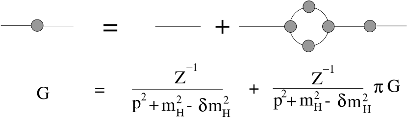
Figure 1: Relation between bare and clothed propagator at one loop.

Now we proceed to set up the computation of the renormalization constants needed in the match between continuum and lattice theories. We begin with the scalar propagator. In the continuum theory the value of the scalar propagator is $G(p^{2})=1/(p^{2}+m_{H}^{2}-\pi_{\Phi,C}(p^{2}))$, with $\pi_{\Phi,C}$ the continuum theory self-energy computed using the clothed vertices and propagators, expressed in lattice units. In the lattice theory the bare propagator is modified by $Z^{-1}_{\Phi}$, so the clothed propagator is (see Figure 1)

$$G=\frac{Z^{-1}_{\Phi}}{p^{2}+m_{HL}^{2}-\delta m_{HL}^{2}}\left(1+\pi_{\Phi,L}G\right)\,,$$ (14)

and hence

$$(Z_{\Phi}-1)p^{2}+(Z_{\phi}-1)m_{HL}^{2}-Z_{\Phi}\delta m_{HL}^{2}=\pi_{\Phi,L}-\pi_{\Phi,C}\,.$$ (15)

Hence one can determine $\delta m_{HL}^{2}$ and $Z_{\Phi}$ from the difference between the lattice and continuum self-energies at $O(p^{0})$ and $O(p^{2})$. The self-energies should be computed using clothed vertices and wave functions, which coincide (by hypothesis) in the infrared; so the difference will be ultraviolet dominated, and here the clothed vertices and wave functions can be replaced by bare ones (without $Z$ and $\delta\lambda$ corrections) with an $O(\beta_{L}^{-1})$ error, which would be accounted for in a full two loop calculation and will only lead to an $O(\beta_{L}^{-2})$ error in $Z_{\Phi}$, and can therefore be neglected. Similarly, the $(Z_{\Phi}-1)m_{HL}^{2}$ can be dropped ($m^{2}_{HL}$ being $O(\beta_{L}^{-2})$), and the $Z_{\Phi}$ in front of $\delta m_{HL}^{2}$ can be set to 1.

Next, denoting the loop contribution to the amputated 1PI four point function at small (zero) external momentum as $-V_{\lambda}$ (the minus sign because the contribution from the scalar self-coupling is $-\lambda$), and again denoting the lattice and continuum values with $L$ and $C$ subscripts respectively, one demands that the actual strength of the scalar self coupling coincide between lattice and continuum theories,

$$(\lambda_{L}-\delta\lambda_{L})Z_{\Phi}^{2}+V_{\lambda,L}=\lambda_{L}+V_{\lambda,C}\,,$$ (16)

and hence, at leading order in $\beta_{L}^{-1}$,

$$\delta\lambda_{L}=V_{\lambda,L}-V_{\lambda,C}+2\lambda(Z_{\Phi}-1)\,.$$ (17)

Again, the $V_{\lambda}$ are computed with the clothed vertices and propagators, but can be computed using the naive bare propagators and vertices because the difference will be ultraviolet dominated.

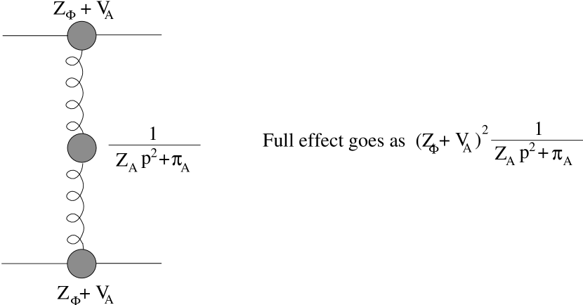
Figure 2: The full influence of a gauge particle propagating between two lines depends on the vertex and propagator renormalizations. Here and throughout SU(2) lines will be curly and U(1) lines will be wiggly.

To find $Z_{A}$ and $Z_{B}$ one must compute not only the gauge field self-energy corrections $\pi_{A}$ and $\pi_{B}$, but also the corrections to the gauge-scalar vertex, which we will denote as $V_{A}$, $V_{B}$. (It does not matter which vertex is considered, by gauge invariance; we choose the scalar vertex because it is the easiest to compute.) $Z_{A}$ should be chosen so that the complete effect of a gauge particle propagating between two lines, say two scalar lines, is the same between the lattice and continuum theories, see Figure 2. The strength of the vertex at each end of the propagator is multiplied by $Z_{\Phi}+V_{A,L}$ in the lattice theory and $1+V_{A,C}$ in the continuum theory; the $Z_{\Phi}$ factor arises because its appearance in the action modifies both the wave function and the coupling to the gauge field. The modification of the propagator is similar to that for the scalar, and we find that to match the full modification (a vertex at each end and a propagator in the middle) we must choose $Z_{A}$ such that

$$\frac{(Z_{\Phi}+V_{A,L})^{2}}{Z_{A}p^{2}-\pi_{A,L}}=\frac{1+V_{A,C}}{p^{2}-\pi_{A,C}}\,,$$ (18)

or, at leading order in $\beta_{L}^{-1}$,

$$Z_{A}-1=2(Z_{\Phi}-1)+2(V_{A,L}-V_{A,C})+\frac{\pi_{A,L}-\pi_{A,C}}{p^{2}}\,.$$ (19)

The equation for $Z_{B}$ is analogous, and in this case the vertex and Higgs wave function contributions will turn out to cancel.

The $\Phi^{2}$ operator multiplicatively renormalizes due to the diagrams shown in Figure 8, because in every diagram where the operator appears on an infrared Higgs field line, there is a corresponding diagram where the $\Phi^{2}$ insertion on that line is replaced with the one loop insertion shown in that figure. If the sum of the contributions of the diagrams there, at small (zero) external momentum, are denoted by $L_{\Phi,L}$, and the continuum contribution is $L_{\Phi,C}$, then the renormalization of the $\Phi^{2}$ operator is

$$Z_{OP}=1-(L_{\Phi,L}-L_{\Phi,C})\,,$$ (20)

where each $L$ should be computed with clothed propagators, vertices, and operator insertions. Again, at the correct value of $Z_{OP}$ the infrared definition of the operator insertions will coincide, so there is no infrared divergent contribution to the difference; the difference is UV dominated and can be computed, at the desired level of accuracy, with the bare vertices and propagators.

It is possible to scale $\Phi$ by a constant $\kappa$ without changing the physics, provided one multiplies $Z_{\Phi}$ by $\kappa^{-2}$ and $Z_{OP}$ by $\kappa^{-2}$. Only the combination $Z_{\Phi}Z_{OP}^{-1}$ must be meaningful and gauge invariant. It is convenient to perform such a scaling of $\Phi$ to set $Z_{OP}$ to 1, in which case one should add $(L_{\Phi,L}-L_{\Phi,C})$ to $Z_{\Phi}$ at the very end of the calculation.

The diagrams needed for the renormalization are presented in the next section, and their values are tabulated there. All but two are performed in lattice Lorentz gauge with a general gauge parameter, to check gauge parameter independence; the exceptions are the gauge field self-energy diagrams with all gauge vertices, which are only performed in Feynman gauge; so we have not yet checked the gauge invariance of $Z_{A}$. The results of the calculation are

$$Z_{A}-1 = \beta_{L}^{-1}\left(\frac{73}{3}\frac{\xi}{4\pi}+\frac{1}{12}\frac{\Sigma}{4\pi}+\frac{1}{3}\right)\,,$$ (21)

$$Z_{B}-1 = \beta_{L}^{-1}\tan^{2}\Theta_{W}\left(-\frac{1}{3}\frac{\xi}{4\pi}+\frac{1}{12}\frac{\Sigma}{4\pi}+\frac{1}{3}\right)\,,$$ (22)

$$Z_{\Phi}Z_{OP}^{-1}-1 = \beta_{L}^{-1}\left((9+3\tan^{2}\Theta_{W}-6\lambda)\frac{\xi}{4\pi}+\frac{3+\tan^{2}\Theta_{W}}{6}\frac{\Sigma}{4\pi}\right)\,,$$ (23)

$$\delta m_{HL}^{2} = \beta_{L}^{-1}(6+2\tan^{2}\Theta_{W}+6\lambda_{L})\frac{\Sigma}{4\pi}\,,$$ (24)

$$\delta\lambda_{L} = \beta_{L}^{-1}\left(\left(-12\lambda_{L}^{2}-4-2(1+\tan^{2}\Theta_{W})^{2}+6\lambda_{L}(3+\tan^{2}\Theta_{W})\right)\frac{\xi}{4\pi}+\right.$$

$$\left.\frac{3+\tan^{2}\Theta_{W}}{3}\lambda_{L}\frac{\Sigma}{4\pi}\right)\,.$$

The constants $\Sigma=3.175911536$ and $\xi=0.152859325$ have the same meaning as in [3], and arise from integrals presented in Appendix A. If one is interested in the theory without the U(1) gauge group, set $\tan^{2}\Theta_{W}=0$ and disregard $Z_{B}$. Equations (21)–(2) are the main result of this paper.

By applying these corrections to the Hamiltonian of a lattice simulation one should be able to remove all $O(a)$ errors (except in the absolute determination of the order parameter and the phase transition temperature, as discussed above). If one already has numerical data, then the $O(a)$ errors can be removed by re-interpreting the meaning of the answers. In the case of SU(2) Higgs theory alone, equating

$$\beta_{naive}\bigg{(}\sum 1-\frac{1}{2}{\rm Tr}P_{ij}+\frac{1}{2}\Phi_{a,naive}D^{2}_{Latt,ab}\Phi_{b,naive}+$$

$$\frac{m_{HL}^{2}-\delta m_{HL}^{2}}{2}\Phi^{2}_{naive}+\frac{\lambda_{L,naive}}{4}(\Phi^{2}_{naive})^{2}\bigg{)}$$ (26)

with

$$\beta_{imp}\bigg{(}Z_{A}\sum 1-\frac{1}{2}{\rm Tr}P_{ij}+\frac{1}{2}Z_{\Phi}\Phi_{a,imp}D^{2}_{Latt,ab}\Phi_{b,imp}+$$

$$Z_{\Phi}\frac{m_{HL}^{2}-\delta m_{HL}^{2}}{2}\Phi^{2}_{imp}+Z_{\Phi}^{2}\frac{\lambda_{L,imp}-\delta\lambda_{L}}{4}(\Phi^{2}_{imp})^{2}\bigg{)}\,,$$ (27)

one finds as matching conditions

$$\beta_{imp} = Z_{A}^{-1}\beta_{naive}\,,$$ (28)

$$\lambda_{L,imp} = Z_{A}^{-1}\lambda_{L,naive}+\delta\lambda_{L}\,,$$ (29)

$$\beta^{2}_{imp}Z_{OP}\Phi^{2}_{imp} = Z_{\Phi}^{-1}Z_{OP}Z_{A}^{-1}\beta_{naive}^{2}\Phi^{2}_{naive}\,.$$ (30)

One should re-interpret at what temperature the simulation was conducted, what input value of $\lambda_{L}$ was used, and what the result for $\beta_{L}^{2}\Phi^{2}$ was. Note both that the value of $\lambda_{L,imp}$ is smaller than the value of $\lambda_{L,naive}$ and that the rescaling of $\beta_{L}^{2}\Phi^{2}$ reduces its value. Both lead to an overestimate (before correction) of the strength of the phase transition, the first because the phase transition is stronger at smaller $\lambda$ and the second because the real jump in the order parameter is smaller than that using naive conversions. The error in $\lambda$ is the most problematic, because at small values of $\lambda$ the strength of the phase transition is strongly $\lambda$ dependent (one loop perturbation theory, which applies here, says the jump in $\Phi^{2}$ should go as $\lambda^{-2}$), and at larger values of $\lambda$ the properties of the phase transition may change qualitatively as one changes $\lambda$. Note also that $Z_{A}-1\simeq 0.65\beta_{L}^{-1}$ is quite large, and so are corrections where $Z_{A}$ appears.

One can get a rough understanding of the magnitudes of $Z_{A}$, $Z_{B}$, $Z_{\Phi}$, and $\delta m_{HL}^{2}$ by considering the tadpole correction scheme of Lepage and Mackenzie [12]. Based on a mean field theory argument, they propose that the dominant loop contributions at every order can be absorbed by making an “educated guess” for the constants $Z_{A}$, etc, as follows: compute the mean value of the trace of an elementary plaquette, and call it $U$ (or $u$ for the U(1) plaquette). Then guess that every term in the action which contains a link should be multiplied by $U^{-1/4}$ (with the value of $U$ found after the correction has been applied, so $U$ must be found self-consistently). Hence, $Z_{A}$ should roughly equal $U^{-1}$, $Z_{\Phi}$ should roughly equal $U^{-1/4}u^{-1/4}$, $Z_{B}$ should roughly equal $u^{-1}$, and $\delta m_{HL}^{2}$ should be about $6(U^{-1/4}u^{-1/4}-1)$ (because the hopping term in the Higgs wave function gets corrected, but not the local term). It is quite easy to compute at one loop that $U=1-\beta_{L}^{-1}$ and $u=1-\tan^{2}\Theta_{W}\beta_{L}^{-1}/3$. (This is just the approximation that the average energy in the plaquette term in the Hamiltonian obeys equipartition.) Hence, one guesses that, at lowest order in $\beta_{L}$,

$$\beta_{L}(Z_{A}-1) \simeq 1\,,$$ (31)

$$\beta_{L}(Z_{B}-1) \simeq \frac{\tan^{2}\theta_{W}}{3}\,,$$ (32)

$$\beta_{L}(Z_{\Phi}Z_{OP}^{-1}-1) \simeq \frac{3+\tan^{2}\Theta_{W}}{12}\,,$$ (33)

$$\beta_{L}\delta m^{2}_{HL} \simeq \frac{3+\tan^{2}\Theta_{W}}{2}\,.$$ (34)

In fact, at $\lambda_{L}=0$, the numerical values of the corrections are

$$\beta_{L}(Z_{A}-1) = 0.65\,,$$ (35)

$$\beta_{L}(Z_{B}-1) = 0.350\tan^{2}\Theta_{W}\,,$$ (36)

$$\beta_{L}(Z_{\Phi}Z_{OP}^{-1}-1) = 0.0786(3+\tan^{2}\Theta_{W})\,,$$ (37)

$$\beta_{L}\delta m^{2}_{HL} = 0.505(3+\tan^{2}\Theta_{W})\,,$$ (38)

which are all close. The tadpole argument is least accurate for the SU(2) wave function correction $Z_{A}-1$.

The tadpole improvement value for the correction to the scalar self-coupling is that it should only change due to the wave function correction. This misses the corrections at even powers of $\lambda_{L}$ (though these are all suppressed by the rather small number $\xi/(4\pi)$). These corrections are important when $\lambda_{L}$ is fairly small, because results are very $\lambda_{L}$ sensitive in this regime. This illustrates a limitation of the tadpole improvement scheme in a theory with non-gauge couplings.

3 Details of the calculation

Here we will present the calculations of the vertices and self-energies needed in the last section in more detail. To illustrate what is involved in the calculation we will present the full details of the contribution of loops involving gauge particles to the scalar self-energy and of scalar loops to the gauge field self-energy. For all other diagrams we will simply present results.

Figure 3: Diagrams contributing to the Higgs boson self-energy. The curly line refers to the SU(2) gauge particle, the wiggly line to the U(1) gauge particle, and the solid line to the scalar.

The diagrams contributing to the Higgs self-energy are presented in Figure 3. Diagram $(a)$ is computed already in [3]. It is straightforward and leads to an $O(p^{0})$ contribution to the difference in self-energies of

$$\pi_{\Phi,L}-\pi_{\Phi,C}=\beta_{L}^{-1}\left(-6\lambda_{L}\frac{\Sigma}{4\pi}\right)\qquad{\rm from}\;(a)\,.$$ (39)

Diagram $(b)$ vanishes in the $\overline{\rm MS}$ regulated continuum theory, so its contribution to the difference of self-energies in Landau gauge is

$$-\frac{3}{\beta_{L}}\int_{\left[-\pi,\pi\right]^{3}}\frac{d^{3}k}{(2\pi)^{3}}\frac{\delta_{ij}\left(\delta_{ij}-\frac{\tilde{k}_{i}\tilde{k}_{j}}{\tilde{k}^{2}}\right)}{\tilde{k}^{2}}\cos p_{i}\,,$$ (40)

where here and throughout $p$ is the momentum of the line, $\tilde{k}_{i}=2\sin(k_{i}/2)$, and $\tilde{k}^{2}=\sum_{i=1,2.3}\tilde{k}_{i}^{2}$. The factor of $3$ is a group factor.

To make expressions more concise, the factor $d^{3}k/(2\pi)^{3}$ will henceforth be implied in every integral, continuum or lattice.

At small $p$, which is the interesting regime, $\cos(p_{i})\simeq 1-p_{i}^{2}/2$, and the contribution from diagram $(b)$ becomes

$$\frac{-3}{\beta_{L}}\int_{\left[-\pi,\pi\right]^{3}}\left(\frac{2}{\tilde{k}^{2}}-\sum_{i}\frac{p_{i}^{2}}{2}\frac{\tilde{k}^{2}-\tilde{k}_{i}^{2}}{(\tilde{k}^{2})^{2}}\right)\,.$$ (41)

The integral of $\tilde{k}_{i}^{2}/(\tilde{k}^{2})^{2}$ is just $1/3$ the integral of $1/\tilde{k}^{2}$ by cubic invariance, so the contribution of the diagram is

$$\pi_{\Phi,L}-\pi_{\Phi,C}=\beta_{L}^{-1}(-6+p^{2})\frac{\Sigma}{4\pi}\qquad{\rm from}\;(b)\,.$$ (42)

The contribution of $(d)$ differs only in counting factors; the $3$ is replaced with $\tan^{2}\Theta_{W}$, which arises from the U(1) propagator.

In Landau gauge, diagram $(c)$ on the lattice contributes

$$\pi_{\Phi,L}\;{\rm from}\;(c)\;=\frac{3}{\beta_{L}}\int_{\left[-\pi,\pi\right]^{3}}\frac{(\widetilde{2p-k})_{i}(\widetilde{2p-k})_{j}\left(\delta_{ij}-\frac{\tilde{k}_{i}\tilde{k}_{j}}{\tilde{k}^{2}}\right)}{\tilde{k}^{2}(\widetilde{p-k})^{2}}\,.$$ (43)

The continuum contribution is

$$\pi_{\Phi,C}\;{\rm from}\;(c)\;=\frac{3}{\beta_{L}}\int_{\Re^{3}}\frac{(2p-k)_{i}(2p-k)_{j}\left(\delta_{ij}-\frac{k_{i}k_{j}}{k^{2}}\right)}{k^{2}(p-k)^{2}}\,.$$ (44)

Each numerator vanishes at $p=0$, so to extract the $O(p^{2})$ behavior we need only expand the numerator to $O(p^{2})$ and use the denominator at $p=0$. (Each contribution is then separately infrared divergent, but the infrared divergences match and do not matter to the difference.) Since

$$(\widetilde{2p-k})_{i}=2\sin(p_{i}-k_{i}/2)=-\tilde{k}_{i}\cos(p_{i})+\widetilde{2p}_{i}\cos(k_{i}/2)\,,$$ (45)

and $\tilde{k}_{i}$ annihilates against the gauge propagator (only because we are in Landau gauge), the contributions simplify at small $p$ to

$$\pi_{\Phi,L}-\pi_{\Phi,C}\;{\rm from}\;(c)\; = \frac{3}{\beta_{L}}\sum_{ij}4p_{i}p_{j}\left(\int_{\left[-\pi,\pi\right]^{3}}\frac{\cos(k_{i}/2)\cos(k_{j}/2)(\delta_{ij}-\tilde{k}_{i}\tilde{k}_{j}/\tilde{k}^{2})}{(\tilde{k}^{2})^{2}}-\right.$$ (46)

$$\left.\int_{\Re^{3}}\frac{\delta_{ij}-k_{i}k_{j}/k^{2}}{k^{4}}\right)\,.$$

Each integral vanishes when $i\neq j$. When $i=j$, one may use $\cos^{2}(k_{i}/2)=1-\tilde{k}_{i}^{2}/4$ and cubic invariance to reorganize the contribution as

$$\pi_{\Phi,L}-\pi_{\Phi,C}\;{\rm from}\;(c)=\frac{3p^{2}}{\beta_{L}}\left[\frac{8}{3}\left(\int_{\left[-\pi,\pi\right]^{3}}\frac{1}{(\tilde{k}^{2})^{2}}-\int_{\Re^{3}}\frac{1}{k^{4}}\right)-\frac{1}{3}\int_{\left[-\pi,\pi\right]^{3}}\frac{1}{\tilde{k}^{2}}+\int_{\left[-\pi,\pi\right]^{3}}\frac{\tilde{k}_{1}^{4}}{(\tilde{k}^{2})^{3}}\right]\,.$$ (47)

The first two integral expressions here are the constants $\xi/4\pi$ and $\Sigma/4\pi$. The last is related to these constants by an identity, Eq. (110). The result is

$$\pi_{\Phi,L}-\pi_{\Phi,C}\;{\rm from}\;(c)\;=\frac{3p^{2}}{\beta_{L}}\left(3\frac{\xi}{4\pi}-\frac{1}{6}\frac{\Sigma}{4\pi}\right)$$ (48)

in Landau gauge. To get the contribution from diagram $(e)$, replace the group factor, $3$, with $\tan^{2}\Theta_{W}$.

In this gauge, the numerical value of the contribution to the wave function renormalization from diagram $(c)$ is $-0.017/\beta_{L}$, while the contribution from the “tadpole” diagram $(b)$ is $+0.253/\beta_{L}$. The tadpole contribution is much bigger, even though diagram $(b)$ vanishes in the continuum theory and would not naively be expected to contribute to the wave function renormalization at all. The contribution of this diagram almost exactly equals the expectation of the “tadpole improvement” argument.

For a general gauge parameter, where the gauge propagator becomes

$$\frac{\delta_{ij}+(\alpha-1)\frac{\tilde{k}_{i}\tilde{k}_{j}}{\tilde{k}^{2}}}{\tilde{k}^{2}}\,,$$ (49)

the contribution from $(b)$ changes by $\alpha(\Sigma/4\pi)(-3+p^{2}/2)$, and the contribution from $(c)$ changes by $-\alpha(\Sigma/4\pi)(-3+p^{2}/2)-3\alpha p^{2}\xi/4\pi$. The mass squared correction is not gauge parameter dependent, but the wave function correction is. This will be matched by a similar gauge parameter dependence in $Z_{OP}$, so the combination $Z_{\Phi}Z_{OP}^{-1}$ is gauge invariant.

Figure 4: Contributions to the SU(2) gauge particle self-energy $\pi_{A}$. The curly line is the gauge particle, the solid line is the scalar, and the dotted line is the ghost.

New complications arise in computing the gauge particle self-energy. The value of the self-energy must be transverse and rotationally invariant, and it must approach zero at $p\rightarrow 0$; but individual diagrams need not separately satisfy these requirements. It is a nontrivial check on the calculation if they do, and on the lattice that check will involve the use of identities, which are intimately related to gauge invariance. To illustrate some of these issues we will present the calculation of the self-energy corrections from scalar loops. Two diagrams contribute, diagrams $(f)$ and $(g)$ in Figure 4. The contribution of $(f)$, which vanishes in the $\overline{\rm MS}$ renormalized continuum theory, is

$$\pi_{A,L}\;{\rm from}\;(f)=-\frac{2}{\beta_{L}}\delta_{AB}\delta_{ij}\int_{\left[-\pi,\pi\right]^{3}}\frac{\cos k_{i}}{\tilde{k}^{2}}\,,$$ (50)

where the 2 arises from the trace over the fundamental representation (in the standard continuum notation it would be 1/2, but here the coupling involves the Pauli matrix $\tau$ rather than $\tau/2$), and the $\delta_{AB}$ is in group space. Using $\cos k_{i}=1-\tilde{k}_{i}^{2}/2$ and cubic invariance, we perform the integrals and get

$$\pi_{A,L}\;{\rm from}\;(f)=-\frac{2}{\beta_{L}}\delta_{AB}\delta_{ij}\left(\frac{\Sigma}{4\pi}-\frac{1}{6}\right)\,.$$ (51)

This does not vanish as $p\rightarrow 0$, and in fact does not depend on $p$ at all. It is also independent of the gauge parameter $\alpha$, because no gauge propagators appear in the loop.

Diagram $(g)$ contributes

$$\pi_{A,L}\;{\rm from}\;(g)=\frac{2}{\beta_{L}}\delta_{AB}\frac{1}{2}\int_{\left[-\pi,\pi\right]^{3}}\frac{(\widetilde{2k})_{i}(\widetilde{2k})_{j}}{(\widetilde{k-p/2})^{2}(\widetilde{k+p/2})^{2}}$$ (52)

in the lattice regulation and

$$\pi_{A,C}\;{\rm from}\;(g)=\frac{2}{\beta_{L}}\delta_{AB}\frac{1}{2}\int_{\Re^{3}}\frac{2k_{i}2k_{j}}{(k-p/2)^{2}(k+p/2)^{2}}-\;{\rm UV\;divergence}$$ (53)

in the continuum. The “$-$UV divergence” subtracts the value at $p=0$. Hence the $O(p^{0})$ contribution is just the lattice value, which is (using $(\widetilde{2k})_{i}=2\tilde{k}_{i}\cos(k_{i}/2)$)

$$\frac{\delta_{AB}}{\beta_{L}}\int_{\left[-\pi,\pi\right]^{3}}\frac{4\tilde{k}_{i}\tilde{k}_{j}\cos(k_{i}/2)\cos(k_{j}/2)}{(\tilde{k}^{2})^{2}}=\frac{\delta_{AB}\delta_{ij}}{\beta_{L}}\int_{\left[-\pi,\pi\right]^{3}}\frac{4\tilde{k}_{1}^{2}-\tilde{k}_{1}^{4}}{(\tilde{k}^{2})^{2}}\,.$$ (54)

The integral involving $\tilde{k}_{1}^{2}$ can be performed using cubic invariance and gives $(4/3)(\Sigma/4\pi)$, but it is not immediately obvious how to perform the other integral, or that its value will correctly cancel the other $O(p^{0})$ parts. The integral is solved using the identity, Eq. (113), which was derived from the invariance of $\int_{\left[-\pi,\pi\right]^{3}}\ln(\tilde{k}^{2})$ on shifting $k_{1}$ (which can be compensated for by a shift in the integration range). It does in fact cancel the other $O(a^{0})$ parts arising from scalar loops.

To understand why, note that all 1 loop contributions to the gauge action from scalar loops can be computed by performing the integral over the Higgs fields in the Gaussian approximation (ie neglecting $\lambda_{L}$); the scalar loop contribution is $(-1/2){\rm Tr\,ln}(-D^{2}+m^{2})$. This can then be expanded about ${\rm Tr}\ln-\partial^{2}+m^{2}=\int_{\left[-\pi,\pi\right]^{3}}\ln(\tilde{k}^{2}+m^{2})$. The required identity came from shifting the integration variable in exactly this integral (at $m^{2}=0$), which is of course the same as applying a spatially nonvarying gauge field. In fact, Eq. (112) contains precisely the integrals in Eqs. (50) and (54) which contribute at $O(p^{0})$.

Expanding the contribution from diagram $(g)$ to $O(p^{2})$ one finds, from Eq. (52),

$$\frac{\delta_{AB}}{\beta_{L}}\int_{\left[-\pi,\pi\right]^{3}}\frac{4\tilde{k}_{i}\tilde{k}_{j}\cos(k_{i}/2)\cos(k_{j}/2)}{(\tilde{k}^{2})^{2}}\left[\sum_{l}\frac{p_{l}^{2}}{2\tilde{k}^{2}}\left(\frac{1}{2}\tilde{k}_{l}^{2}-1\right)+\right.$$

$$\left.\sum_{lm}p_{l}p_{m}\frac{\tilde{k}_{l}\tilde{k}_{m}\cos(k_{l}/2)\cos(k_{m}/2)}{(\tilde{k}^{2})^{2}}\right]\,.$$ (55)

The corresponding continuum contribution is

$$\frac{\delta_{AB}}{\beta_{L}}\int_{\Re^{3}}\frac{4k_{i}k_{j}}{k^{4}}\left[-\frac{p^{2}}{2k^{2}}+\frac{(p\cdot k)^{2}}{k^{4}}\right]\,,$$ (56)

which removes the infrared divergence of the lattice version. The difference between the lattice and continuum expressions must be of form

$$\frac{\delta_{AB}}{\beta_{L}}(A\delta_{ij}p^{2}+Bp_{i}p_{j}+C\delta_{ij}p_{i}^{2})\,,$$ (57)

simply from cubic invariance. We expect that the answer will be rotationally invariant and transverse, $B=-A$ and $C=0$, because all gauge invariant, cubic invariant, dimension 4 operators are; and this will constitute a check on the calculation. The $p_{1}^{2}$ contribution when $i=j=1$ is

$$A+B+C=4\int_{\left[-\pi,\pi\right]^{3}}\frac{\tilde{k}_{1}^{2}(1-\tilde{k}_{1}^{2}/4)}{(\tilde{k}^{2})^{2}}\left(\frac{\tilde{k}_{1}^{2}-2}{4\tilde{k}^{2}}+\frac{\tilde{k}_{1}^{2}(1-\tilde{k}_{1}^{2}/4)}{(\tilde{k}^{2})^{2}}\right)-\;{\rm IR\;divergence}\,,$$ (58)

which can be evaluated using Eq. (115) and Eq. (120) in Appendix A; it vanishes. One can find $A$ from the $p_{2}^{2}$ contribution when $i=j=1$; it equals

$$A=4\int_{\left[-\pi,\pi\right]^{3}}\frac{\tilde{k}_{1}^{2}(1-\tilde{k}_{1}^{2}/4)}{(\tilde{k}^{2})^{2}}\left(\frac{\tilde{k}_{2}^{2}-2}{4\tilde{k}^{2}}+\frac{\tilde{k}_{2}^{2}(1-\tilde{k}_{2}^{2}/4)}{(\tilde{k}^{2})^{2}}\right)-\;{\rm IR\;divergence}\,,$$ (59)

which can be evaluated using Eq. (116) and Eq. (121), and equals

$$A=\frac{1}{12}\frac{\Sigma}{4\pi}-\frac{1}{3}\frac{\xi}{4\pi}\,.$$ (60)

To evaluate B one takes the $p_{1}p_{2}$ part when $i=1$ and $j=2$, which is

$$B=8\int_{\left[-\pi,\pi\right]^{3}}\frac{\tilde{k}_{1}^{2}\tilde{k}_{2}^{2}(1-\tilde{k}_{1}^{2}/4)(1-\tilde{k}_{2}^{2}/4)}{(\tilde{k}^{2})^{4}}-\;{\rm IR\;divergence}=-A\,,$$ (61)

evaluating it with the same equations. Hence $C=0$ and the result is indeed rotationally invariant and transverse.

There are no new techniques involved in the remaining integrals, so we will simply tabulate all of the results here.

Five diagrams, $(a)$ through $(e)$ of Figure 3, contribute to the Higgs self-energy. They are evaluated above, and equal

$$\beta_{L}(\pi_{\Phi,L}-\pi_{\Phi,C}) = -6\lambda\frac{\Sigma}{4\pi}\quad{\rm from}\;(a)\quad+$$ (66)

$$(-6-3\alpha)\frac{\Sigma}{4\pi}+p^{2}(1+\frac{\alpha}{2})\frac{\Sigma}{4\pi}\quad{\rm from}\;(b)\quad+$$

$$3\alpha\frac{\Sigma}{4\pi}+p^{2}\left((-\frac{1}{2}-\frac{\alpha}{2})\frac{\Sigma}{4\pi}+(9-3\alpha)\frac{\xi}{4\pi}\right)\quad{\rm from}\;(c)\quad+$$

$$\left[(-2-\alpha)\frac{\Sigma}{4\pi}+p^{2}(\frac{1}{3}+\frac{\alpha}{6})\frac{\Sigma}{4\pi}\right]\tan^{2}\Theta_{W}\quad{\rm from}\;(d)\quad+$$

$$\left[\alpha\frac{\Sigma}{4\pi}+p^{2}\left((-\frac{1}{6}-\frac{\alpha}{6})\frac{\Sigma}{4\pi}+(3-\alpha)\frac{\xi}{4\pi}\right)\right]\tan^{2}\Theta_{W}\quad{\rm from}\;(e)\,.$$

Seven diagrams, $(f)$ through $(l)$ of Figure 4, contribute to the SU(2) field self-energy. In Feynman ($\alpha=1$) gauge, they contribute ($\delta_{AB}$ understood)

$$\beta_{L}(\pi_{A,L}-\pi_{A,C}) = \delta_{ij}\left(-2\frac{\Sigma}{4\pi}+\frac{1}{3}\right)\quad{\rm from}\;(f)\quad+$$

$$\delta_{ij}\left(2\frac{\Sigma}{4\pi}-\frac{1}{3}\right)+(\delta_{ij}p^{2}-p_{i}p_{j})\left(\frac{1}{12}\frac{\Sigma}{4\pi}-\frac{1}{3}\frac{\xi}{4\pi}\right){\rm from}\;(g)\quad+$$

$$\frac{-2}{3}\delta_{ij}\qquad{\rm from}\;(h)\qquad+$$

$$\frac{-4}{9}\delta_{ij}\qquad{\rm from}\;(i)\qquad+$$

$$\delta_{ij}\left(-4\frac{\Sigma}{4\pi}+\frac{2}{3}\right)+\delta_{ij}p^{2}\left(-\frac{1}{6}\frac{\Sigma}{4\pi}+\frac{2}{3}\frac{\xi}{4\pi}\right)$$

$$+p_{i}p_{j}\left(\frac{1}{6}\frac{\Sigma}{4\pi}+\frac{4}{3}\frac{\xi}{4\pi}\right)\quad{\rm from}\;(j)+$$ (73)

$$\delta_{ij}\left(-16\frac{\Sigma}{4\pi}+\frac{28}{9}\right)+\delta_{ij}p^{2}\left(\frac{14}{3}\frac{\Sigma}{4\pi}\right)+$$

$$\quad p_{i}p_{j}\left(-\frac{8}{3}\frac{\Sigma}{4\pi}-\frac{1}{3}\right)+\delta_{ij}p_{i}^{2}\left(-2\frac{\Sigma}{4\pi}+\frac{1}{3}\right)\quad{\rm from}\;(k)\quad+$$

$$\delta_{ij}\left(20\frac{\Sigma}{4\pi}-\frac{4}{3}\right)+\delta_{ij}p^{2}\left(14\frac{\xi}{4\pi}-\frac{29}{6}\frac{\Sigma}{4\pi}+\frac{1}{3}\right)+$$

$$\quad p_{i}p_{j}\left(-16\frac{\xi}{4\pi}+\frac{17}{6}\frac{\Sigma}{4\pi}\right)+\delta_{ij}p_{i}^{2}\left(2\frac{\Sigma}{4\pi}-\frac{1}{3}\right)\quad{\rm from}\;(l)\,.$$

Only the last two are gauge parameter dependent. The total is rotationally invariant, transverse, and free of $O(p^{0})$ contributions.

Figure 5: Contributions to the U(1) particle self-energy. The wiggly lines are the U(1) gauge particle, and the straight lines are the scalars. Diagram $(o)$ only exists in the lattice theory.

Only three diagrams, $(m)$ through $(o)$ in Figure 5, contribute to $\pi_{B}$. Scalar loops contribute the same value as for the SU(2) self-energy, because although the SU(2) contribution is enhanced by a group factor of 2, the SU(2) doublet contains 2 fields which are charged under U(1). The result is

$$\frac{\beta_{L}}{\tan^{2}\Theta_{W}}(\pi_{B,L}-\pi_{B,C}) = \delta_{ij}\left(-2\frac{\Sigma}{4\pi}+\frac{1}{3}\right)\quad{\rm from}\;(m)\quad+$$ (76)

$$\delta_{ij}\left(2\frac{\Sigma}{4\pi}-\frac{1}{3}\right)+(\delta_{ij}p^{2}-p_{i}p_{j})\times$$

$$\left(\frac{1}{12}\frac{\Sigma}{4\pi}-\frac{1}{3}\frac{\xi}{4\pi}\right)\quad{\rm from}\;(n)\quad+$$

$$\frac{1}{3}(\delta_{ij}p^{2}-p_{i}p_{j})\qquad{\rm from}\;(o)$$

The factor of $\tan^{2}\Theta_{W}$ arises as follows. Each $B$ field propagator contributes a $\tan^{2}\Theta_{W}$, and there is 1 more propagator when a self-energy insertion occurs than when none occurs; in the case of diagram $(o)$, there are two extra propagators, but the vertex contributes $\tan^{-2}\Theta_{W}$. Although this diagram does not exist in the continuum theory, it completely dominates the contribution to the self-energy. It arises from the compact nature of the gauge action, and its value is given exactly by the tadpole improvement technique at one loop.

Figure 6: Contributions to the scalar 4-point function, which correct $\lambda_{L}$. All but $(p)$ and $(q)$ vanish in Landau gauge. The curly lines are SU(2) gauge propagators, the wiggly lines are U(1) gauge propagators.

Some 12 diagrams contribute to the scalar four point vertex, in a general gauge. All but 4 of these vanish in Landau gauge; also the diagrams involving gauge lines can be grouped by topology, with the type of gauge particle ($A$ or $B$) only determining counting factors. The diagrams are listed in Figure 6; their contributions are

$$\beta_{L}(V_{\lambda,L}-V_{\lambda,C}) = -12\lambda^{2}\frac{\xi}{4\pi}\quad{\rm from}\;(p)\quad+$$ (81)

$$-(4+2(1+\tan^{2}\Theta_{W})^{2})\frac{\xi}{4\pi}+$$

$$-(2+(1+\tan^{2}\Theta_{W})^{2})\alpha^{2}\frac{\xi}{4\pi}\quad{\rm from}\;(q)\quad+$$

$$2(2+(1+\tan^{2}\Theta_{W})^{2})\alpha^{2}\frac{\xi}{4\pi}\quad{\rm from}\;(r)\quad+$$

$$-(2+(1+\tan^{2}\Theta_{W})^{2})\alpha^{2}\frac{\xi}{4\pi}\quad{\rm from}\;(s)\quad+$$

$$(6+2\tan^{2}\Theta_{W})\alpha\frac{\xi}{4\pi}\lambda\quad{\rm from}\;(t)\,.$$

The $\alpha^{2}$ terms all cancel, and the $\alpha$ term absorbs the $\alpha$ term in $Z_{\Phi}$ in the computation of $\delta\lambda_{L}$. The Landau gauge value could have been derived by inserting $m^{2}$ in the propagators of the “tadpole” contributions to the scalar self-energy and finding the $O(m^{2})$ term, or equivalently by expanding the (tadpole) one loop contribution to the Landau gauge effective potential to a sufficient power in $m$, as discussed in Appendix A.

Figure 7: Contributions to the SU(2) Higgs vertex. The wiggly lines are U(1) propagators, the curly ones are SU(2) propagators, the straight ones are scalar propagators. The last two diagrams vanish on integration over the loop momenta.

Seven diagrams contribute to the scalar-$A$ field 3 point vertex. Again, they can be grouped by topology; they are presented in Figure 7. Their contributions are

$$\beta_{L}(V_{A,L}-V_{A,C}) = \left(\frac{5}{3}+\tan^{2}\Theta_{W}\right)\left(-\frac{1}{3}-\frac{\alpha}{6}\right)\frac{\Sigma}{4\pi}\quad{\rm from}\;(u)\quad+$$ (85)

$$\left(1+\tan^{2}\Theta_{W}\right)\left(-3\frac{\xi}{4\pi}+\frac{1}{6}\frac{\Sigma}{4\pi}+\frac{\alpha}{3}\frac{\Sigma}{4\pi}\right)\quad{\rm from}\;(v)\quad+$$

$$\left(-1+\tan^{2}\Theta_{W}\right)\left(\alpha\frac{\xi}{4\pi}-\frac{\alpha}{6}\frac{\Sigma}{4\pi}\right)\quad{\rm from}\;(w)\quad+$$

$$\left(3\alpha\frac{\xi}{4\pi}-\frac{\alpha}{6}\frac{\Sigma}{4\pi}\right)\quad{\rm from}\;(x)\,.$$

When using this result to get $Z_{A}$ one must remember that the $A$ field self-energy was only evaluated at $\alpha=1$; note that there is a nonzero $\alpha$ dependence in $V_{A}+\pi_{\Phi}$, and hence also in $\pi_{A}$.

The diagrams contributing to $V_{B}$ are the same as $(u)$ through $(w)$, but with $A$ and $B$ lines switched. The contributions are

$$\beta_{L}(V_{B,L}-V_{B,C}) = (3+\tan^{2}\Theta_{W})\left(-\frac{1}{3}-\frac{\alpha}{6}\right)\frac{\Sigma}{4\pi}\quad{\rm from}\;(u)\quad+$$ (88)

$$(3+\tan^{2}\Theta_{W})\left(-3\frac{\xi}{4\pi}+\frac{1}{6}\frac{\Sigma}{4\pi}+\frac{\alpha}{3}\frac{\Sigma}{4\pi}\right)\quad{\rm from}\;(v)\quad+$$

$$(3+\tan^{2}\Theta_{W})\left(\alpha\frac{\xi}{4\pi}-\frac{\alpha}{6}\frac{\Sigma}{4\pi}\right)\quad{\rm from}\;(w)\,.$$

The total is precisely minus the total $O(p^{2})$ contribution to the Higgs self-energy; hence $V_{B}$ and $Z_{\Phi}$ cancel in the evaluation of $Z_{B}$ and only $\pi_{B}$ contributes. The same thing happens in the renormalization of continuum, 4 dimensional U(1) gauge theory.

Figure 8: Contributions to the $\Phi^{2}$ operator renormalization. The dots are $\Phi^{2}$ operators, the plain lines are scalar propagators, the curly line is the SU(2) propagator, and the wiggly line is the U(1) propagator. The diagrams with gauge particles automatically vanish (at zero momentum) in Landau gauge.

Finally, there are three contributions to the multiplicative renormalization of the $\Phi^{2}$ operator insertion, listed in Figure 8. The contributions to $L_{\Phi}$ are

$$\beta_{L}(L_{\Phi,L}-L_{\Phi,C}) = -6\lambda\frac{\xi}{4\pi}\quad{\rm from}\;(y)\quad+$$ (90)

$$\alpha\left(3+\tan^{2}\Theta_{W}\right)\frac{\xi}{4\pi}\quad{\rm from}\;(z)\,,$$

which will cancel the $\alpha$ dependence in $Z_{\Phi}$ when one forms the gauge invariant combination $Z_{\Phi}Z_{OP}^{-1}$.

This concludes the evaluation of the relevant diagrams.

4 Conclusion

We have argued that the substantial linear in $a$ corrections arising in lattice Monte-Carlo investigations of the strength of the electroweak phase transition arise from the difference between ultraviolet screening of couplings and wave functions in the continuum and lattice theories, and can be cured either with an $O(a)$ shift in the relation between the continuum and lattice couplings and wave functions or equivalently with an $O(a)$ shift in the interpretation of lattice data (the values of $\lambda$ and $\beta_{L}$ used and the jumps in order parameters).

     

Figure 9: Jump in $\beta_{L}^{2}\Phi^{2}$ as a function of scalar self-coupling, before $O(a)$ corrections (squares) and after $O(a)$ corrections (triangles). The data is that used in [6]. The figure at the left is the $m_{H}^{*}=35$GeV data, at $\beta_{L}=8,12,20$ (from top to bottom before improvement and from small $\lambda$ to large $\lambda$ after), and the figure at the right is the $m_{H}^{*}=60$GeV data, at $\beta_{L}=5,8,12,20$. In each case the last unimproved datapoint is the result of a linear extrapolation of the others.

To test the technique, we re-examine existing data, the infinite volume extrapolations of the jump in the order parameter $\Delta(\beta_{L}^{2}\Phi^{2})$ (the difference of $\Phi^{2}$ between phases at the equilibrium temperature, extrapolated to the infinite volume limit) for $m^{*}_{H}=35$ and $60$GeV, computed in [6]. We applied $O(a)$ corrections to the data using Eqs. (28)–(30). We plot the uncorrected and corrected jumps in the order parameter in Figure 9, which also shows the two loop perturbative value as a function of $\lambda$. The corrected data tell a consistent story. At $m^{*}_{H}=35$GeV the two loop perturbation theory is working fairly well, underestimating somewhat the jump in the order parameter, presumably because of transition strengthening three loop effects [6] (though the coarsest lattice seems inconsistent with the other two, but see below), and at $60$GeV the jump is beginning to fall below the perturbative prediction. Before the improvement the points demand a substantial extrapolation; the result of this extrapolation is also shown in the figure. Such an extrapolation should successfully remove $O(a)$ errors, but it is less optimal than improving the lattice data analytically because the extrapolation is numerically expensive due to the demands of the finest lattices, and the errors are dominated by the $O(a^{2})$ errors in the coarsest lattice (which may also be amplified by the extrapolation process) and the statistical errors in the finest lattice. Using a single intermediate coarseness lattice and the $O(a)$ improvements could give smaller statistical and systematic errors at less numerical cost.

For the $m^{*}_{H}=35$GeV data the linear extrapolation of the uncorrected data is quite poor, with $\chi^{2}=2.9$ for 1 degree of freedom. Comparing the corrected data to the perturbative estimate, we see that the two finer lattices are following the expected trend of decreasing $\phi$ with increasing $\lambda$; but the data on the coarsest lattice buck the trend, suggesting that the blame for the poor fit falls on the data from the coarsest lattice ($\beta_{L}=8$). This is probably due to $O(a^{2})$ effects. At such a small value of $\lambda$, the phase transition is very strong, and the particle masses in the broken phase are quite large. The natural scale of the physics involved in the phase transition is quite short, short enough that one should worry about corrections from high dimension operators. We can estimate the size of such corrections by seeing how much one such effect, a $\phi^{5}/\beta_{L}^{2}$ term induced in the effective potential at one loop by nonrenormalizable derivative corrections (computed in Appendix A), changes the perturbative value. Its contribution to the effective potential, summing only over the transverse gauge fields, is

$$\frac{6}{160\pi\beta_{L}^{2}}\left(\Phi^{2}\right)^{5/2}\,,\;{\rm lattice\;units\,,}\qquad{\rm or}\;\;\frac{6}{160\pi}\frac{g^{5}a^{2}T}{32}\phi^{5}\,,\;{\rm physical\;units}\,.$$ (91)

Adding this to the 2 loop effective potential shifts the minimum (in the lattice units used in the figure) from $\beta_{L}^{2}\Phi^{2}=35.4$ to $\beta_{L}^{2}\Phi^{2}=30.2$, which is of the right sign and the right general size to account for the discrepancy between the data and the perturbative value. (This is not the only $O(a^{2})$ effect, so we should not have expected good agreement after correction–it can only be used to estimate what accuracy we can expect.) The correction for the next datapoint is already smaller by a factor of $0.4$. Because of this error, the extrapolation of the unimproved data suggest a jump in the order parameter which is larger than the perturbative value, by an amount which is inconsistent with the corrected data from the two finer lattices. This is an example of the danger of linear extrapolations; $O(a^{2})$ systematic errors from the coarsest lattice data appear in the final answer, which depends very strongly on the coarse lattice data because its statistical errorbars are small.

The $O(a^{2})$ correction from nonrenormalizable operators is smaller for the $60$GeV data, because a $\phi^{5}$ term changes the strength of the phase transition far more for small $\lambda$ than for large $\lambda$; from the one loop perturbative effective potential we would estimate the fractional change in the order parameter $\phi$ due to such a term to be $\propto\phi/\lambda\sim 1/\lambda^{2}$. A small value of $\lambda$ demands a very fine lattice, which makes intuitive sense because a stronger phase transition involves physics on shorter length scales. Hence, the extrapolation of the $60$GeV data much better represents the trend in the improved data.

The technique we have presented here is not restricted to correcting the jump in the order parameter $\Phi^{2}$. One can also correct computed surface tensions, by replacing the naive values of $\beta_{L}$ and $\lambda$ with the corrected versions in those calculations. Improving the surface tension calculation is particularly easy because it only depends on a physical length scale and ratios of probabilities for different values of the order parameter, and not on any operator insertion which might renormalize. To remove $O(a)$ errors from the calculation of other order parameters, such as the string bit or the Wilson loop, one must still compute the one loop corrections to the appropriate operator insertions.

While we estimate the size of an $O(a^{2})$ error above, so far we have said nothing about removing $O(a^{2})$ errors. These arise not only from the finite renormalization of the bare couplings and wave functions, but from tree level nonrenormalizable operators, which modify the infrared behavior of the theory at $O(a^{2})$ (for instance, the $\phi^{5}$ term mentioned above). To remove them one should start out with an “improved” action [13], rather than the minimal Wilson action we discuss here. Unfortunately the ultraviolet effects computed here will be different in such an improved action and must be recomputed.

This still leaves out the $O(a^{2})$ corrections to couplings and wave functions which arise from two loop graphs. Directly computing these would involve 205 two loop diagrams for SU(2) Higgs theory, and even more if the U(1) factor is included. It is clearly impractical to attempt this renormalization. However, one can absorb the great majority of the $O(a^{2})$ corrections to wave functions and couplings in a very economical fashion, by using the tadpole improvement scheme. First, the action is tadpole improved by the technique developed by Lepage and Mackenzie [12], thereby correcting most of the loop contributions to the wave functions and couplings, at every order. Then $O(a)$ corrections to the wave functions and couplings are applied, to compensate for the difference between the full $O(a)$ corrections and those $O(a)$ corrections which the tadpole scheme will have already made. This removes all $O(a)$ errors and most $O(a^{2})$ and higher order errors.

Note finally that while removing all $O(a^{2})$ errors may be impossible in practice, removing all $O(a^{3})$ errors is probably impossible even in principle, because there are $O(a^{2})$ corrections to the ultraviolet propagators, brought about by their couplings to infrared nonperturbative physics, which are not computable and which propagate via the one loop UV corrections discussed here into $O(a^{3})$ errors in the infrared wave functions and propagators. However, from a pragmatic point of view, since the dimensional reduction program itself has a limited accuracy, and since it is quite easy in practice to drive $O(a^{3})$ corrections below the $1\%$ level, this is not of practical importance.

Acknowledgements

I would like to thank Kari Rummukainen for providing the data presented in the conclusion, and Peter Lepage and Keijo Kajantie for useful conversations and correspondence.

Appendix A Integrals and Identities

In this appendix we expand the tadpole integral in powers of mass, evaluating two of the resulting integrals numerically. Then we derive a number of identities which relate all other integrals needed in this paper to these two.

The basic integral encountered in finding the effective potential to one loop in the lattice regulation with the minimal (Wilson) action is [3]

$$aI(m)=\int_{\left[-\pi,\pi\right]^{3}}\frac{d^{3}k}{(2\pi)^{3}}\frac{1}{\tilde{k}^{2}+(am)^{2}}\,,$$ (92)

where, as in the text, $\tilde{k}_{i}=2\sin(k_{i}/2)$ and $\tilde{k}^{2}=\sum_{i=1,2,3}4\sin^{2}(k_{i}/2)$. Also, the $d^{3}k/(2\pi)^{3}$ will be assumed in all integrals in the remainder of the section for notational simplicity. The integral has been expanded in a power series about $am=0$ through $O((am)^{3})$ in [3]. We repeat that expansion here, but show exactly what integral is responsible for the third and fourth coefficients, rather than getting them numerically by evaluating the original integral. This is useful because the integral for one coefficient arises in the one loop renormalization performed in the text, and the other illustrates the influence of nonrenormalizable operators on the infrared physics.

The integral is well behaved about $k=0$ and so to lowest order in $am\ll 1$ it is

$$\int_{\left[-\pi,\pi\right]^{3}}\frac{1}{\tilde{k}^{2}}=\frac{\Sigma}{4\pi}\,,\qquad\Sigma=3.175911536\,.$$ (93)

The notation is borrowed from Farakos et. al. [3], who found an analytic expression (although the value presented above is the result of an accurate numerical integration). This gives the (divergent) mass squared correction.

Adding and subtracting this integral, we get

$$aI(m)=\frac{\Sigma}{4\pi}-\int_{\left[-\pi,\pi\right]^{3}}\frac{(am)^{2}}{\tilde{k}^{2}(\tilde{k}^{2}+(am)^{2})}\,.$$ (94)

The second integral is infrared dominated, and it is best to add and subtract the analogous continuum integral, which can be performed;

$$\int_{\left[-\pi,\pi\right]^{3}}\frac{(am)^{2}}{\tilde{k}^{2}(\tilde{k}^{2}+(am)^{2})} = \int_{\Re^{3}}\frac{(am)^{2}}{k^{2}(k^{2}+(am)^{2})}+$$

$$\int_{\left[-\pi,\pi\right]^{3}}\left(\frac{(am)^{2}}{\tilde{k}^{2}(\tilde{k}^{2}+(am)^{2})}-\frac{(am)^{2}}{k^{2}(k^{2}+(am)^{2})}\right)-$$

$$\int_{\Re^{3}-\left[-\pi,\pi\right]^{3}}\frac{(am)^{2}}{k^{2}(k^{2}+(am)^{2})}\,,$$

$$\int_{\Re^{3}}\frac{(am)^{2}}{k^{2}(k^{2}+(am)^{2})} = \frac{am}{4\pi}\,.$$ (96)

This gives the famous negative cubic term in the effective potential, and leaves a remainder which vanishes as $(am)^{2}$.

Because $k^{2}-\tilde{k}^{2}=O(k^{4})$ at small $k$, the remaining terms are well behaved about $k=0$, and we can again extract the dominant behavior by adding and subtracting the values at $am=0$:

$$\!\!\!\!\!\!\!\int_{\left[-\pi,\pi\right]^{3}}\left(\frac{(am)^{2}}{\tilde{k}^{2}(\tilde{k}^{2}+(am)^{2})}-\frac{(am)^{2}}{k^{2}(k^{2}+(am)^{2})}\right)-\int_{\Re^{3}-\left[-\pi,\pi\right]^{3}}\frac{(am)^{2}}{k^{2}(k^{2}+(am)^{2})}=$$

$$\!\!\!\!\!\!\!(am)^{2}\left[\int_{\left[-\pi,\pi\right]^{3}}\left(\frac{1}{(\tilde{k}^{2})^{2}}-\frac{1}{k^{4}}\right)-\int_{\Re^{3}-\left[-\pi,\pi\right]^{3}}\frac{1}{k^{4}}\right]-(am)^{4}\times$$ (97)

$$\!\!\!\!\!\!\!\left[\int_{\left[-\pi,\pi\right]^{3}}\left(\frac{1}{(\tilde{k}^{2})^{2}(\tilde{k}^{2}+(am)^{2})}-\frac{1}{k^{4}(k^{2}+(am)^{2})}\right)-\int_{\Re^{3}-\left[-\pi,\pi\right]^{3}}\frac{1}{k^{4}(k^{2}+(am)^{2})}\right]$$ (98)

Following the notation of [3] we denote the first integral as

$$\left[\int_{\left[-\pi,\pi\right]^{3}}\left(\frac{1}{(\tilde{k}^{2})^{2}}-\frac{1}{k^{4}}\right)-\int_{\Re^{3}-\left[-\pi,\pi\right]^{3}}\frac{1}{k^{4}}\right]=\frac{\xi}{4\pi}\,.$$ (99)

To evaluate it numerically we reduce the second integral to a single integral over a polar angle,

$$\int_{\Re^{3}-\left[-\pi,\pi\right]^{3}}\frac{1}{k^{4}}=\frac{1}{4\pi^{3}}+\frac{1}{\pi^{4}}\int_{0}^{\pi/4}\cos(\theta)\arctan(\cos(\theta))d\theta=0.0134035706$$ (100)

and perform the first numerically, directly. The result is $\xi=0.152859325$. This enters the coefficient of an $O(a)$ contribution to the effective potential which behaves as $\phi^{4}$; summing over species, one can derive $V_{\lambda}$ in Landau gauge.

Finally, Eq. (98) is infrared dominated and $O((am)^{3})$, because $k^{2}-\tilde{k}^{2}$ is order $k^{4}$ at small $k$. To extract this infrared $O((am)^{3})$ piece one should expand $\tilde{k}^{2}$ to $O(k^{4})$,

$$\sum_{i}4\sin(k_{i}/2)=\sum_{i}k_{i}^{2}-\frac{1}{12}\sum_{i}k_{i}^{4}\,,$$ (101)

from which it follows that the contribution $-$Eq. (98) to the effective potential is approximately

$$(am)^{4}\int_{\Re^{3}}\sum_{i}k_{i}^{4}\left(\frac{2k^{2}+(am)^{2}}{k^{4}(k^{2}+(am)^{2})^{2}}-\frac{2}{k^{6}}\right)$$ (102)

$$= \frac{(am)^{3}}{32\pi}\,.$$

This generates an $O(a^{2})$ term in the effective potential of form $\phi^{5}$ and is caused by the (tree level) nonrenormalizable derivative terms in the action arising from the choice of lattice regulation. Had the expansion of $\tilde{k}^{2}$ been free of the $O(k^{4})$ part, no such term would appear and the first one loop effect beyond the $O(a)$ correction to $\lambda$ would be an $O(a^{3})$ induced nonrenormalizable $\phi^{6}$ term. (Of course, there would still be corrections arising at two loops, for instance an $O(a^{2})$ correction to $\lambda$.)

The result for the tadpole integral is then

$$aI(m)=\frac{\Sigma}{4\pi}-\frac{am}{4\pi}-\frac{\xi(am)^{2}}{4\pi}+\frac{(am)^{3}}{32\pi}+O((am)^{4})\,,$$ (103)

and the contribution to the effective potential, $\int mI(m)dm,$ is

$$\frac{\Sigma}{4\pi a}\frac{m^{2}}{2}-\frac{m^{3}}{12\pi}-\frac{\xi m^{4}a}{16\pi}+\frac{a^{2}m^{5}}{160\pi}+O(a^{3}m^{6})\,.$$ (104)

The first term is the linearly divergent mass squared correction. The second is the negative cubic term which makes the phase transition first order, the third is the contribution to the $O(a)$ correction $V_{\lambda}$, and the fourth is a change induced at one loop from a nonrenormalizable derivative correction operator which appears with $O(a^{2})$ coefficient at tree level in the lattice theory. Of these, the terms with $\Sigma$ and $\xi$ in them arise from integrals which we need in the body of the text.

Several other integrals arise in the calculations in the text, but a number of identities relate them all to the two (numerical) integrals, Eq. (93) and Eq. (99). Some of these identities involve trigonometric manipulations of numerators, for instance using $\cos^{2}(k_{i}/2)=1-\tilde{k}_{i}^{2}/4$ and $\cos(k_{i})=1-\tilde{k}_{i}^{2}/2$; we will not bother to list these here. Some use cubic invariance;

$$\int_{\left[-\pi,\pi\right]^{3}}\frac{\tilde{k}_{1}^{2}}{(\tilde{k}^{2})^{2}}=\frac{1}{3}\int_{\left[-\pi,\pi\right]^{3}}\frac{\tilde{k}_{1}^{2}+\tilde{k}_{2}^{2}+\tilde{k}_{3}^{2}}{(\tilde{k}^{2})^{2}}=\frac{1}{3}\int_{\left[-\pi,\pi\right]^{3}}\frac{1}{\tilde{k}^{2}}=\frac{1}{3}\frac{\Sigma}{4\pi}\,.$$ (105)

Similarly,

$$\int_{\left[-\pi,\pi\right]^{3}}\frac{\tilde{k}_{1}^{2}}{\tilde{k}^{2}}=\frac{1}{3}$$ (106)

and

$$\int_{\left[-\pi,\pi\right]^{3}}\frac{\tilde{k}_{1}^{2}}{(\tilde{k}^{2})^{3}}-\;{\rm continuum\;version}\;=\frac{1}{3}\frac{\xi}{4\pi}\,.$$ (107)

Here “- continuum version” means that $k_{1}^{2}/k^{6}$ should be subtracted from the integrand and the integral of $k_{1}^{2}/k^{6}$ outside the first Brillion zone should also be subtracted. In what follows the meaning will be analogous.

Cubic invariance cannot be used to evaluate the integral over $\tilde{k}_{i}^{4}/(\tilde{k}^{2})^{3}$. To do so we must take advantage of the periodicity of the integrand on $2\pi$ shifts in any $k_{i}$. For $\epsilon$ an infinitesimal, the periodicity of $\tilde{k}_{1}^{2}$ ensures that

$$\int_{\left[-\pi,\pi\right]^{3}}\frac{1}{\tilde{k}^{2}}=\int_{\left[-\pi,\pi\right]^{3}}\frac{1}{(2\sin^{2}((k_{1}+\epsilon)/2))^{2}+\tilde{k}_{2}^{2}+\tilde{k}_{3}^{2}}\,.$$ (108)

Now, excising a small neighborhood about the origin to avoid the singularity there, one can expand in $\epsilon$. At order $\epsilon^{2}$, one finds after some work that

$$0=\int_{\left[-\pi,\pi\right]^{3}-{\rm excision}}\left(-\frac{1}{(\tilde{k}^{2})^{2}}+\frac{1}{2}\frac{\tilde{k}_{1}^{2}}{(\tilde{k}^{2})^{3}}+4\frac{\tilde{k}_{1}^{2}}{(\tilde{k}^{2})^{3}}-\frac{\tilde{k}_{1}^{4}}{(\tilde{k}^{2})^{3}}\right)+\;{\rm surface\;term}\,,$$ (109)

where the surface term arises on the boundary of the excised region. It cancels the linear infrared divergence occurring from the two terms with $O(1/k^{4})$ infrared behavior, so what remains is the difference between these terms and their continuum analogs, eg $\int 1/(\tilde{k}^{2})^{2}$ becomes Eq. (99). Using the previous integrals and identities we can integrate all but the last term, so we find that

$$\int_{\left[-\pi,\pi\right]^{3}}\frac{\tilde{k}_{1}^{4}}{(\tilde{k}^{2})^{3}}=\frac{1}{6}\frac{\Sigma}{4\pi}+\frac{1}{3}\frac{\xi}{4\pi}\,.$$ (110)

Because $\tilde{k}_{1}^{2}+\tilde{k}_{2}^{2}+\tilde{k}_{3}^{2}=\tilde{k}^{2}$, it follows from this integral, Eq. (105), and cubic invariance that

$$\int_{\left[-\pi,\pi\right]^{3}}\frac{\tilde{k}_{1}^{2}\tilde{k}_{2}^{2}}{(\tilde{k}^{2})^{3}}=\frac{1}{12}\frac{\Sigma}{4\pi}-\frac{1}{6}\frac{\xi}{4\pi}\,.$$ (111)

Repeating the above technique, but starting with the integral over $\ln(\tilde{k}^{2})$ rather than $1/\tilde{k}^{2}$, one finds that

$$0=\int_{\left[-\pi,\pi\right]^{3}}\frac{-2\tilde{k}^{2}+\tilde{k}^{2}\tilde{k}_{1}^{2}+4\tilde{k}_{1}^{2}-\tilde{k}_{1}^{4}}{(\tilde{k}^{2})^{2}}\,,$$ (112)

or

$$\int_{\left[-\pi,\pi\right]^{3}}\frac{\tilde{k}_{1}^{4}}{(\tilde{k}^{2})^{2}}=\frac{1}{3}-\frac{2}{3}\frac{\Sigma}{4\pi}\,,$$ (113)

and hence also

$$\int_{\left[-\pi,\pi\right]^{3}}\frac{\tilde{k}_{1}^{2}\tilde{k}_{2}^{2}}{(\tilde{k}^{2})^{2}}=\frac{1}{3}\frac{\Sigma}{4\pi}\,.$$ (114)

Continuing the expansion to fourth order in $\epsilon$, and using the previously derived identities, one obtains after considerable algebra that

$$\int_{\left[-\pi,\pi\right]^{3}}\frac{\tilde{k}_{1}^{4}(1-\tilde{k}_{1}^{2}/4)^{2}}{(\tilde{k}^{2})^{4}}-\;{\rm continuum\;version}-$$

$$\int_{\left[-\pi,\pi\right]^{3}}\frac{\tilde{k}_{1}^{2}(1-\tilde{k}_{1}^{2}/2)(1-\tilde{k}_{1}^{2}/4)}{(\tilde{k}^{2})^{3}}-\;{\rm continuum\;version} = -\frac{1}{48}+\frac{1}{8}\frac{\Sigma}{4\pi}-\frac{1}{8}\frac{\xi}{4\pi}\,.$$ (115)

Shifting the $k_{2}$ integral by $\delta$, the condition that the $O(\epsilon^{2}\delta^{2})$ term should vanish gives that

$$3\int_{\left[-\pi,\pi\right]^{3}}\frac{\tilde{k}_{1}^{2}\tilde{k}_{2}^{2}(1-\tilde{k}_{1}^{2}/4)(1-\tilde{k}_{2}^{2}/4)}{(\tilde{k}^{2})^{4}}-\;{\rm continuum\;version}-$$

$$\int_{\left[-\pi,\pi\right]^{3}}\frac{\tilde{k}_{1}^{2}(1-\tilde{k}_{2}^{2}/2)(1-\tilde{k}_{1}^{2}/4)}{(\tilde{k}^{2})^{3}}-\;{\rm continuum\;version} = \frac{1}{32}\frac{\Sigma}{4\pi}-\frac{1}{8}\frac{\xi}{4\pi}\,.$$ (116)

By shifting $k_{1}$ by $\epsilon$ in the integral

$$\int_{\left[-\pi,\pi\right]^{3}}\frac{\tilde{k}_{2}^{2}}{\tilde{k}^{2}}$$ (117)

and expanding to second order in $\epsilon$, one finds using Eq. (114) that

$$\int_{\left[-\pi,\pi\right]^{3}}\frac{\tilde{k}_{1}^{4}\tilde{k}_{2}^{2}}{(\tilde{k}^{2})^{3}}=\frac{1}{6}\frac{\Sigma}{4\pi}-\frac{2}{3}\frac{\xi}{4\pi}\,,$$ (118)

and hence

$$\int_{\left[-\pi,\pi\right]^{3}}\frac{\tilde{k}_{1}^{6}}{(\tilde{k}^{2})^{3}}=\frac{1}{3}-\frac{\Sigma}{4\pi}+\frac{4}{3}\frac{\xi}{4\pi}\,,$$ (119)

by applying the same technique used to get Eq. (111) and using Eq. (113). With these integrals we can derive that

$$\int_{\left[-\pi,\pi\right]^{3}}\frac{\tilde{k}_{1}^{2}(1-\tilde{k}_{1}^{2}/2)(1-\tilde{k}_{1}^{2}/4)}{(\tilde{k}^{2})^{3}}-\;{\rm continuum\;version}=\frac{1}{24}-\frac{1}{4}\frac{\Sigma}{4\pi}+\frac{1}{4}\frac{\xi}{4\pi}\,,$$ (120)

and

$$\int_{\left[-\pi,\pi\right]^{3}}\frac{\tilde{k}_{1}^{2}(1-\tilde{k}_{2}^{2}/2)(1-\tilde{k}_{1}^{2}/4)}{(\tilde{k}^{2})^{3}}-\;{\rm continuum\;version}=-\frac{1}{16}\frac{\Sigma}{4\pi}+\frac{1}{4}\frac{\xi}{4\pi}\,.$$ (121)

Hence we know the value of each integral in Eqs. (115) and (116) separately.

No other identities are needed for to complete the 1 loop renormalization.

Appendix B Feynman rules

Most of the Feynman rules needed in the calculation appear in [14]; the measure insertion (diagram $(h)$ in Section 3) is smaller by a factor of $2/3$ from the one printed there, which is for SU(3) rather than SU(2), and similarly in the four point vertex in Eq. (14.44) one must set $d_{ABC}$ to 0 and the $(2/3)$ in front of $\delta_{AB}\delta_{BC}+\delta_{AC}\delta_{BD}+\ldots$ should become $1$. Our conventions for the scale and the gauge wave function mean $a$ should be replaced by $1$ and $g$ by $2$ everywhere. Also, the sign for the ghost coupling to two gauge particles is backwards there.

What remains are the scalar propagator and the vertices involving the scalar. The propagator, in the ultraviolet where $m$ is negligible, is just $\delta_{ab}/p^{2}$. The 4-point vertex is

$$-2\lambda(\delta_{ab}\delta_{cd}+\delta_{ac}\delta_{bd}+\delta_{ad}\delta_{bc})$$ (122)

where $a,b,c,d$ are the species types of the incoming lines. The vertices involving gauge particles, and the pure U(1) four point vertex, are given in Figures 10 to 12. The notation is that $(i)_{ab}$ means the action of $i$ on the species type, eg species type 1 becomes type 2 and type 2 becomes $-$ type 1, etc. Any $i$ by itself is the imaginary number which arises when one Fourier transforms an odd function. The vertices in Figure 12 do not have continuum analogs. Their role in generating extra tadpole diagrams is quite important on the lattice; for instance they dominate the corrections $V_{B}$ to the U(1)- Higgs vertex.

Figure 10: Feynman rules for the U(1) four point function and the three point gauge-Higgs couplings.

Figure 11: Feynman rules for the four point gauge-Higgs couplings.

Figure 12: Feynman rules for the five point gauge-Higgs couplings.

Appendix C Results in other theories

Here we present results for the renormalization of the abelian Higgs model with $N$ scalars, and for SU(2)$\times$U(1) theory with adjoint scalars (the Weinberg-Salaam model after dimensional reduction but before integrating out heavy modes).

The action of the 3-D abelian Higgs model on a lattice is

$$\sum_{x}\left[Z_{B}\sum_{i<j}(1-{\rm Re}\>p_{ij})+Z_{\Phi}\sum_{b=1}^{N}\sum_{i}\left(\Phi_{b}^{2}(x)-\Phi_{ab}(x)u_{iac}(x)\Phi_{cb}(x+i)\right)+\right.$$

$$\left.Z_{\Phi}\frac{m_{HL}^{2}}{2}(\sum_{b}\Phi_{b}^{2})+Z_{\Phi}^{2}\frac{\lambda_{L}}{4}(\sum_{b}\Phi^{2}_{b})^{2}\right]\,.$$ (123)

Here $a$ and $c$ are indicies over the real and imaginary part, which are implicitly summed over when $\Phi^{2}$ appears, and $b$ is an index over the $N$ scalar species, which are assumed to have the same mass squared and an $SU(N)$ symmetric quartic interaction. The finite $a$ renormalization only involves diagrams computed already in the text; the results are

$$\beta_{L}\delta\lambda_{L} = \frac{\lambda_{L}}{3}\frac{\Sigma}{4\pi}+\left(6\lambda_{L}-(8+2N)\lambda_{L}^{2}-2\right)\frac{\xi}{4\pi}\,,$$ (124)

$$\beta_{L}(Z_{B}-1) = \frac{1}{3}+N\left(\frac{1}{24}\frac{\Sigma}{4\pi}-\frac{1}{6}\frac{\xi}{4\pi}\right)\,,$$ (125)

$$\beta_{L}\delta m^{2}_{HL} = \left(2+(2+2N)\lambda_{L})\right)\frac{\Sigma}{4\pi}\,,$$ (126)

$$\beta_{L}(Z_{\Phi}Z_{OP}^{-1}-1) = \left(3-(2+2N)\lambda_{L})\right)\frac{\xi}{4\pi}+\frac{1}{6}\frac{\Sigma}{4\pi}\,.$$ (127)

Next we consider SU(2)$\times$U(1) theory, with an adjoint SU(2) scalar $A_{0}$ and an adjoint U(1) scalar $B_{0}$. If one is interested in very high precision calculations of the electroweak phase transition strength one must include these, because the integration over these fields (the so called heavy modes) is lower precision than the integration over the nonzero Matsubara frequencies (the superheavy modes).

The integration over the nonzero Matsubara frequencies generates mass terms for these modes. Interaction terms already exist at tree level, and new ones are generated at one loop in the dimensional reduction. The new mass terms will be denoted $m_{A}^{2}$ and $m_{B}^{2}$, and the new interaction terms in the Lagrangian are

$$\frac{\lambda_{A}}{4}(A_{0}^{2})^{2}+\frac{\lambda_{B}}{4}(B_{0}^{2})^{2}+\frac{h_{A}}{4}\Phi^{2}A_{0}^{2}+\frac{h_{B}}{4}\Phi^{2}B_{0}^{2}+\frac{h_{AB}}{4}A_{0}^{2}B_{0}^{2}+\frac{h^{\prime}}{2}B_{0}\Phi_{a}(-A_{0}\cdot\tau)_{ab}\Phi_{b}\,.$$ (128)

In the minimal standard model, at lowest order in $\alpha_{W}$, the bare values for the new couplings, in lattice units, are [4]

$$\lambda_{AL} = 0\,,$$ (129)

$$\lambda_{BL} = 0\,,$$ (130)

$$h_{AL} = 2\,,$$ (131)

$$h_{BL} = 2\tan^{2}\Theta_{W}\,,$$ (132)

$$h_{ABL} = 0\,,$$ (133)

$$h^{\prime}_{L} = 2\tan\Theta_{W}\,,$$ (134)

but in what follows we will treat the general problem in which their values are arbitrary. Computing the $O(a)$ renormalizations involves no topologically new diagrams, only combinatorics. The couplings and wave functions presented in Section 2 are modified by

$$\frac{1}{3}\frac{\Sigma}{4\pi}-\frac{4}{3}\frac{\xi}{4\pi} {\rm added\;to} \beta_{L}(Z_{A}-1)\,,$$ (135)

$$-\frac{3}{4}h_{AL}^{2}-\frac{1}{4}h_{BL}^{2}-\frac{1}{2}h{{}^{\prime}}_{L}^{2} {\rm added\;to} \beta_{L}\delta\lambda_{L}\,,$$ (136)

$$\frac{3}{2}h_{AL}+\frac{1}{2}h_{BL} {\rm added\;to} \beta_{L}\delta m_{HL}^{2}\,.$$ (137)

The corrections to $Z_{B}$ and $Z_{\Phi}$ vanish.

We denote the new wave function corrections as $Z_{A0}$ and $Z_{B0}$; the notations for the coupling corrections are obvious. The new couplings and wave functions renormalize by

$$\beta_{L}(Z_{A0}-1) = 24\frac{\xi}{4\pi}+\frac{4}{3}\frac{\Sigma}{4\pi}-5\lambda_{AL}\frac{\xi}{4\pi}\,,$$ (138)

$$\beta_{L}(Z_{B0}-1) = -3\lambda_{BL}\frac{\xi}{4\pi}\,,$$ (139)

$$\beta_{L}\delta m_{AL}^{2} = \left(16+5\lambda_{L}+2h_{AL}+\frac{1}{2}h_{ABL}\right)\frac{\Sigma}{4\pi}\,,$$ (140)

$$\beta_{L}\delta m_{BL}^{2} = \left(3\lambda_{BL}+2h_{BL}+\frac{3}{2}h_{ABL}\right)\frac{\Sigma}{4\pi}\,,$$ (141)

$$\beta_{L}\delta\lambda_{AL} = -\left(32+11\lambda_{AL}^{2}+h_{AL}^{2}+\frac{1}{4}h_{ABL}^{2}\right)\frac{\xi}{4\pi}+\lambda_{AL}\left(48\frac{\xi}{4\pi}+\frac{8}{3}\frac{\Sigma}{4\pi}\right)\,,$$ (142)

$$\beta_{L}\delta\lambda_{BL} = -\left(10\lambda_{BL}^{2}+h_{BL}^{2}+\frac{3}{4}h_{ABL}^{2}\right)\frac{\xi}{4\pi}\,,$$ (143)

$$\beta_{L}\delta h_{AL} = -\left(8+6\lambda_{L}h_{AL}+5\lambda_{AL}h_{AL}+2h^{2}_{AL}+\frac{1}{2}h_{BL}h_{ABL}+2h^{\prime 2}_{L}\right)\frac{\xi}{4\pi}+$$ (144)

$$h_{AL}\left((33+3\tan^{2}\Theta_{W})\frac{\xi}{4\pi}+(\frac{11}{6}+\frac{1}{6}\tan^{2}\Theta_{W})\frac{\Sigma}{4\pi}\right)\,,$$

$$\beta_{L}\delta h_{BL} = -\left(6\lambda_{L}h_{BL}+3\lambda_{BL}h_{BL}+2h_{BL}^{2}+\frac{3}{2}h_{AL}h_{ABL}+2h{{}^{\prime}}_{L}^{2}\right)+$$ (145)

$$h_{BL}\left((9+3\tan^{2}\Theta_{W})\frac{\xi}{4\pi}+(\frac{3+\tan^{2}\Theta_{W}}{6})\frac{\Sigma}{4\pi}\right)\,,$$

$$\beta_{L}\delta h_{ABL} = -\left(5\lambda_{AL}h_{ABL}+3\lambda_{BL}h_{ABL}+2h^{2}_{ABL}+2h_{AL}h_{BL}+2h^{\prime 2}_{L}\right)+$$ (146)

$$h_{ABL}\left(24\frac{\xi}{4\pi}+\frac{4}{3}\frac{\Sigma}{4\pi}\right)\,,$$

$$\beta_{L}\delta h^{\prime}_{L} = h^{\prime}_{L}\left(\left(-2\lambda_{L}-h_{AL}-h_{BL}-h_{ABL}+21+3\tan^{2}\Theta_{W}\right)\frac{\xi}{4\pi}+\right.$$ (147)

$$\left.\frac{7+\tan^{2}\Theta_{W}}{6}\frac{\Sigma}{4\pi}\right)\,.$$

Here the wave functions already include corrections to make the operator insertions have their naive normalization. In fact the operator insertions will be mixed by a matrix with $O(a)$ off diagonal terms; what we use above are the diagonal components of the matrix. The off diagonal terms would only be important if the $A_{0}$ or $B_{0}$ fields took on significant condensates at the phase transition, which they should not, because in the realistic case they should be given substantial (Debye) masses. They would also be important if we were interested in the jumps in these condensates, but this is also not of interest. We have not computed the off diagonal terms here.

References

- [1] P. Arnold and O. Espinoza, Phys. Rev. D 47 (1993) 3546; Z. Fodor and A. Hebecker, Nucl. Phys. B 432 (1994) 127.
- [2] K. Kajantie, K. Rummukainen, and M. Shaposhnikov, Nucl. Phys. B 407 (1993) 356; K. Farakos, K. Kajantie, K. Rummukainen, and M. Shaposhnikov, Nucl. Phys. B 425 (1994) 67.
- [3] K. Farakos, K. Kajantie, K. Rummukainen, and M. Shaposhnikov, Nucl. Phys. B 442 (1995) 317.
- [4] K. Kajantie, M. Laine, K. Rummukainen, and M. Shaposhnikov, Nucl. Phys. B 458 (1996) 90.
- [5] K. Farakos, K. Kajantie, K. Rummukainen, and M. Shaposhnikov, Phys. Lett. B 336 (1994) 194; K. Farakos, K. Kajantie, M. Laine, K. Rummukainen, and M. Shaposhnikov, Nucl. Phys. B (Proc. Suppl.) 17 (1996) 705.
- [6] K. Kajantie, M. Laine, K. Rummukainen, and M. Shaposhnikov, Nucl. Phys. B 466 (1996) 189.
- [7] K. Kajantie, M. Laine, K. Rummukainen, and M. Shaposhnikov, Phys. Rev. Lett. 77 (1996) 2887.
- [8] E. Ilgenfritz, J. Kripfganz, H. Perlt, and A. Schiller, Phys. Lett. B 356 (1995) 561; M. Gurtler, E. Ilgenfritz, J. Kripfganz, H. Perlt, and A. Schiller, hep-lat/9512022; hep-lat/9605042.
- [9] F. Karsch, T. Neuhaus, A. Patkos, and J. Rank, Nucl. Phys. B 474 (1996) 217.
- [10] O. Philipsen, M. Teper, and H. Wittig, Nucl. Phys. B 469 (1996), 445; hep-lat/9608067.
- [11] M. Laine, Nucl. Phys. B 451 (1995) 484.
- [12] G. P. Lepage and P. Mackenzie, Phys. Rev. D 48 (1993) 2250.
- [13] P. Weisz, Nucl. Phys. B 212 (1983), 1; G. Curci, P. Menotti, and G. Paffuti, Phys. Lett. B 130 (1983), 205.
- [14] H. J. Rothe, “Lattice Gauge Theories: an Introduction” (World Scientific, Singapore, 1992).