NEW RESULTS ON TOPOLOGICAL SUSCEPTIBILITY IN SU(3) GAUGE THEORY

We survey recent lattice results on QCD topological properties. The behaviour of the topological susceptibility at the deconfining phase transition has been determined. This advance has been made possible by an i) an improvement of the topological charge operator and ii) a non-perturbative determination of renormalizations.

1 Introduction

Relevant progress in the study of topological properties of QCD has been made possible by two recent developments in lattice gauge theories:
1) Improvement of the operators $\!{}^{{\bf?}}$.
2) Non perturbative determination of the renormalizations $\!{}^{{\bf?}}$.

To clarify the meaning of 1) we recall that the building block of lattice gauge theories is the link, $U_{\mu}(\vec{n})=\exp({iaA_{\mu}(\vec{n})})$, or parallel transport from the site $\vec{n}$ of discretized spacetime to the neighbouring site in the direction $\hat{\mu}$, $\vec{n}+a\hat{\mu}$ ($a$ is the lattice spacing). All the operators are constructed in terms of links, and therefore contain arbitrarily high powers of $a\,A_{\mu}$. The identification with continuum is usually done by requiring that the leading order in the power expansion of the lattice operator $O_{L}$ concides with its continuum counter-part $O$

$$O_{L}=Oa^{d}+{\cal O}(a^{d+1})$$ (1)

$d$ is the dimension of the operator. Higher order terms in eq. (1) can be changed with large arbitrariness.

For the action, for example, eq. (1) reads

$$S_{L}=-{1\over 4}G_{\mu\nu}G^{\mu\nu}a^{4}+{\cal O}(a^{6})$$ (2)

Wilson’s action $S_{L}^{W}=\beta\left(1-1/3\;{\rm Re}\;{\rm Tr}\Box\right)$ obeys eq. (2).

The idea of improvement consists in exploiting the arbitrariness in higher order terms to reduce lattice artifacts. Improving the action can make the lattice larger in physical units $\!{}^{{\bf?}}$. Our approach will be to keep the usual Wilson action and to improve the operator $Q_{L}$ for the topological charge $\!{}^{{\bf?}}$, to reduce renormalizations from lattice to continuum. Renormalizations will be determined non perturbatively $\!{}^{{\bf?},{\bf?},{\bf?}}$.

2 Topology in QCD.

The key relation is the anomaly of the singlet axial current

$$\partial^{\mu}j^{5}_{\mu}=2N_{f}Q(x)$$ (3)

where

$$j^{5}_{\mu}=\sum_{f}\bar{\psi_{f}}\gamma_{\mu}\gamma^{5}\psi_{f}$$ (4)

$f$ means flavour, and $N_{f}$ number of flavours. $Q(x)$ is the topological charge density

$$Q(x)={{g^{2}}\over{64\pi^{2}}}\epsilon^{\mu\nu\rho\sigma}G^{a}_{\mu\nu}(x)G^{a}_{\rho\sigma}(x).$$ (5)

The anomaly can explain the magnitude of the $\eta^{\prime}$ mass (the so called $U(1)$ problem $\!{}^{{\bf?}}$) if the topological susceptibility of the vacuum in the quenched approximation (leading order in $1\over{N_{c}}$ expansion)

$$\chi\equiv\int d^{4}x\langle 0|T(Q(x)Q(0))|0\rangle.$$ (6)

is large enough. Quantitatively $\!{}^{{\bf?},{\bf?}}$

$${{2N_{f}}\over{f_{\pi}^{2}}}\chi=m_{\eta}^{2}+m_{\eta^{\prime}}^{2}-2m_{K}^{2}.$$ (7)

Testing eq. (7) is a check at the same time of QCD and of the $1\over{N_{c}}$ expansion, and can be done on the lattice.

The behaviour of $\chi$ at the deconfining temperature is also an important test of models of QCD vacuum $\!{}^{{\bf?}}$.

Another use of eq. (3) which can be made on the lattice is the measurement of the singlet axial charge of the nucleon, $G_{1}(0)$, which is given by $\!{}^{{\bf?}}$

$$G_{1}(0)\simeq\lim_{\vec{p}\rightarrow\vec{p}^{\prime}}{N_{f}\over M_{p}}{{\langle\vec{p}^{\prime}s^{\prime}|Q|\vec{p}s\rangle}\over{\bar{u}_{s^{\prime}}(\vec{p}^{\prime})\gamma^{5}u_{s}(\vec{p})}}$$ (8)

$G_{1}$ is usually related to the quark spin content of the proton $\!{}^{{\bf?}}$.

3 Topology on the lattice.

A lattice version of the topological charge density operator is

$$Q_{L}(x)={{-1}\over{2^{9}\pi^{2}}}\sum_{\mu\nu\rho\sigma=\pm 1}^{\pm 4}{\tilde{\epsilon}}_{\mu\nu\rho\sigma}\hbox{Tr}\left(\Pi_{\mu\nu}(x)\Pi_{\rho\sigma}(x)\right).$$ (9)

In the formal limit $a\rightarrow 0$, in accordance with eq. (1)

$$Q_{L}(x)=a^{4}\,Q(x)+{\cal O}(a^{6}).$$ (10)

Any other choice for $Q_{L}$ will differ from (9) by ${\cal O}(a^{6})$.

$Q_{L}(x)$ renormalizes multiplicatively

$$Q_{L}(x)\simeq_{\beta\rightarrow\infty}Z(\beta)Q(x)a(\beta)^{4}+{\cal O}(a^{6})$$ (11)

Similarly, for the lattice topological susceptibility, defined as

$$\chi_{L}\equiv\langle\sum_{x}Q_{L}(x)Q_{L}(0)\rangle,$$ (12)

we have $\!{}^{{\bf?}}$

$$\chi_{L} = {}_{\beta\to\infty}Z(\beta)^{2}\,a(\beta)^{4}\,\chi+M(\beta)$$ (13)

$$M(\beta) \equiv B(\beta)\langle G_{2}\rangle+P(\beta)\langle{\bf 1}\rangle+{\cal O}(a^{6})$$

where $G_{2}$ is the trace of the energy-momentum tensor and 1 is the identity operator. The presence of $M(\beta)$ is due to the fact that the lattice regularization does not obey the prescription for the singularity at $x=0$ which defines $\chi$ of eq. (6, 7) $\!{}^{{\bf?},{\bf?}}$. From eq.(3)

$$\chi={{\chi_{L}-M(\beta)}\over{Z^{2}a^{4}}}.$$ (14)

$\chi_{L}$ is determined numerically on the lattice. $P(\beta)$, $Z(\beta)$ and $B(\beta)$ depend on the choice of $Q_{L}$, i.e. on the specification of the terms ${\cal O}(a^{6})$ in eq. (10). A good choice gives a small $M(\beta)$ and $Z\approx 1$, so that in eq. (14) $\chi\approx\chi_{L}$ and lattice artifacts are a small part of the numerical determination.

To determine $Z$, $Q_{L}\equiv\int{\rm d}^{4}xQ_{L}(x)\equiv Z\,Q$ is measured on an ensemble of configurations with a definite value of $Q$. A one instanton configuration is heated to dress it with short range quantum fluctuations. The number of instantons is checked step by step $\!{}^{{\bf?}}$, and the configurations in which either the initial instanton has disappeared or new instantons have been created are discarded from the sample (Fig. 1). $M(\beta)$ is determined by measuring $\chi_{L}$ on an ensemble of configurations with $Q=0$ (0 instantons plus quantum fluctuations). Here again the global topological charge is checked step by step and configurations in which it has been changed in the heating procedure are discarded (Fig. 2). We have used an improved operator obtained from $Q_{L}(x)$ by successive smearings, and which differs from it by terms ${\cal O}(a^{6})$ $\!{}^{{\bf?}}$.

Figure 3 shows the plateaux reached by heating 1 instanton and the $Z$’s for the 0, 1 and 2 improved operators.

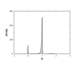
Figure 1: Distribution of topological charge $Q$ for a set of 2000 configurations obtained by 15 heat-bath updatings of a 1-instanton configuration. $\beta=5.75$.

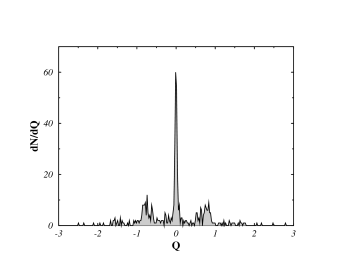
Figure 2: Distribution of topological charge $Q$ for a set of 500 configurations obtained by 36 heat-bath updatings of the zero field configuration. $\beta=5.90$.

The analogous behaviour for $M(\beta)$ is shown in Figure 4. Improving twice the operator produces a factor of 3 in $Z$, or a factor of 10 in $Z^{2}$, and a factor of 10 reduction of $M(\beta)$. The ratio between the physical signal and the lattice artifacts is then improved by 2 orders of magnitude going from the 0 to the 2 smeared operator, and the subtraction in eq. (14) becomes of the order of 10% of $\chi_{L}$ in the scaling window.

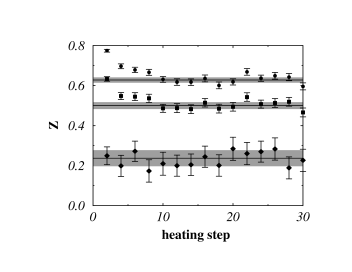
Figure 3: Determination of $Z$ by heating of a 1 instanton configuration. Diamonds, squares and circles correspond to 0, 1 and 2 smearings respectively. $\beta=6.36$.

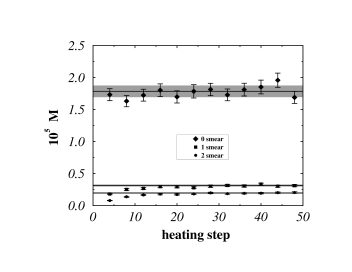
Figure 4: Determination of $M(\beta)$ by heating of the flat configuration. Diamonds, squares and circles correspond to 0, 1 and 2 smearings respectively. $\beta=6.30$.

Figure 5 shows the result for $\chi$ at $T=0$ determined with the 0, 1 and 2 smeared operators: they agree with each other, scale properly and confirm previous results in favour of the Witten-Veneziano mechanism $\!{}^{{\bf?},{\bf?}}$.

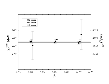
Figure 5: Determination of $\chi$ at $T=0$. Diamonds, squares and circles correspond to 0, 1 and 2 smearings respectively.

Figure 6 shows a new result, which has been made possible by the improvement: the behaviour of $\chi$ across $T_{c}$. The $\chi$ drops by at least one order of magnitude at $T_{c}$. This result can provide an important check of models of QCD vacuum $\!{}^{{\bf?}}$.

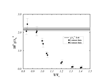
Figure 6: Determination of $\chi$ at $T\not=0$. Circles and squares correspond to 1 and 2 smearings respectively. The horizontal line is the $T=0$ result.

Difficulties are encountered in thermalizing the topological charge with the hybrid Monte Carlo algorithm in full QCD $\!{}^{{\bf?}}$ (Figs. 7,8,9): we are, however, implementing a multicanonical algorithm in which the quark mass is used as a new variable in the Monte Carlo, to exploit the fact that for high quark masses this difficulty is less severe. The procedure works, so that the same technique described here will soon allow the determination of $\chi$, $\chi^{\prime}$ in full QCD and the measurement of the spin content of the proton.

Figure 7: Time history, in units of molecular dynamics time, of the topological charge $Q$ for a hybrid Monte Carlo simulation at $\beta=5.35$ and $a\,m=0.01$.

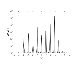
Figure 8: Distribution of values of $Q$ in a sample of 1000 configurations in full QCD obtained with the hybrid Monte Carlo algorithm. $\langle Q\rangle\not=0$ and the distribution is not symmetric under $Q\to-Q$ in contrast with what happens with usual heat bath algorithms for quenched QCD, see Fig. 9.

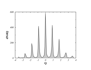
Figure 9: Distribution of values of $Q$ in quenched QCD obtained with the heat bath algorithm.

References

References

- [1] C. Christou, A. Di Giacomo, H. Panagopoulos, E. Vicari, Phys. Rev. D 53, 2619 (1996).
- [2] A. Di Giacomo, E. Vicari, Phys. Lett. B 275, 429 (1992).
- [3] G. P. Lepage, Nucl. Phys. B (Proc. Suppl.) 47, 3 (1996).
- [4] B. Allés, M. Campostrini, A, Di Giacomo, Y. Gündüç, E. Vicari, Phys. Rev. D 48, 2284 (1993)
- [5] B. Allés, M. Campostrini, A, Di Giacomo, Y. Gündüç, E. Vicari, Nucl. Phys. B (Proc. Suppl.) 34 504 (1994).
- [6] S. Weinberg, Phys. Rev. D 11, 3583 (1975).
- [7] E. Witten, Nucl. Phys. B 156, 269 (1979).
- [8] G. Veneziano, Nucl. Phys. B 159, 213 (1979).
- [9] E. Shuryak, Comments in Nuclear and Particle Physics 21, 235 (1994).
- [10] J. E. Mandula, Phys. Rev. Lett. 65, 1403 (1990).
- [11] J. Ellis, I. Karliner, Phys. Lett. B 313, 213 (1993).
- [12] M. Campostrini, A. Di Giacomo, H. Panagopoulos, E. Vicari, Nucl. Phys. B 329, 683 (1990).
- [13] B. Allés, M. D’Elia, A. Di Giacomo, hep-lat/9605013.
- [14] B. Allés, G. Boyd, M. D’Elia, A. Di Giacomo, E. Vicari, hep-lat/9607049, to appear in Phys. Lett. B.